1. Introduction
Underwater acoustic source localization determines the altitude or depth, range, and bearing angle of the underwater target, that is, the three coordinates of the underwater target in the elliptical coordinate system [
1]. The estimation of bearing angle (or direction of arrival (DOA)) of underwater acoustic source is an important and indispensable step in underwater acoustic source localization. In fact, in some underwater acoustic source localization methods, it is the target direction information that is used to estimate the target distance [
2]. Using a vector hydrophone (or vector hydrophone array) is perhaps one of the simplest and most straightforward methods of underwater acoustic source DOA estimation. The vector hydrophone is capable of simultaneously measuring sound pressure and particle velocity along one to three orthogonal directions. Therefore, only a single vector hydrophone can generate a directional beam pattern. A Directional Autonomous Seafloor Acoustic Recorder (DASAR) system consisting of several vector hydrophones has been reported [
3]. By using a vector hydrophone, directional industrial noise is effectively suppressed, and weak marine mammal sounds can be successfully detected.
Conventional beamforming (or delay-and-sum beamforming) is also one of the common DOA estimation methods [
4,
5,
6]. Based on the ray-path approximation for the sound channel’s impulse response, the frequency-difference beamforming method for the sparse hydrophone array is proposed in [
7,
8], which can estimate the signal phase difference by using the conventional delay-and-sum beamforming of the field product at the difference frequency. In contrast, by determining the array weight coefficients in a nonlinear manner, the minimum variance distortionless response (MVDR) method can achieve higher angular resolution than conventional beamforming [
4]. In order to cope with the model mismatch problems in the uncertain ocean environment, such as the signal look direction mismatch, the signal spatial signature mismatch due to local scattering or wavefront distortion [
9,
10], many robust MVDR-based adaptive beamforming algorithms have been proposed [
10,
11,
12].
Similar to the MVDR-based methods, the subspace-based high-resolution DOA estimation techniques also use information carried by the covariance matrix. The most representative subspace-based DOA estimation methods may be the Multiple Signal Classification (MUSIC) algorithm [
13], the Estimation of Signal Parameters via Rotational Invariance Technique (ESPRIT) [
14], and the Propagator Method (PM) [
15]. The key to the subspace-based DOA estimation methods is the estimation of the signal subspace (or noise subspace). To achieve this purpose, one can first perform eigendecomposition on the sample covariance matrix, then construct the signal subspace with the eigenvectors corresponding to the larger eigenvalues, and form the noise subspace with the eigenvectors corresponding to the smaller eigenvalues. Another more sophisticated approach is to reconstruct the sample covariance matrix according to the Toeplitz structure of the covariance matrix [
16], and then obtain the signal subspace in a similar way as above. In contrast to the above eigenvalue-based methods, the eigenvector pruning algorithm implements the estimation of the signal subspace by using the statistical properties of eigenvectors of signal-free sample covariance matrix [
17].
In many underwater acoustic source DOA estimation scenarios, the number of acoustic sources distributed in the underwater far field is much smaller than the number of hydrophones in the observation array. This is the intrinsic basis of the popular sparse-based DOA estimation methods. In the least absolute shrinkage and selection operator (LASSO) method [
18], the signal amplitude vector is obtained by solving an
-norm regularized least-squares problem. The LASSO method contains the
-norm constraint on the solution vector, thus making the result of the solution vector sparse [
19]. By linear transformation of the solution vector, the weighted LASSO method [
20] imposes certain structural constraint on the solution vector to achieve efficient processing of spatially extended sources (e.g., underwater embedded objects in acoustic imaging [
21]). The total variation norm regularization method [
22] for DOA estimation of spatially extended sources can be seen as a special case of the weighted LASSO method, which uses the band matrix to realize the linear transformation of the solution vector, so that the solution vector has block sparsity [
19,
23]. Besides, using the information contained in the covariance matrix, the sparse spectrum fitting (SpSF) algorithm [
24] first performs a vectorization operation on the covariance matrix, and then fits the estimated covariance matrix and the ideal covariance matrix under the
-norm. At the same time, considering the sparsity of the source,
-norm penalization is imposed on the source strength vector. However, SpSF algorithm is based on the assumption that ambient noise is white Gaussian noise. Therefore, Yang L., Yang Y. X., and Wang Y. proposed the directional noise field sparse spectrum fitting (DN-SpSF) algorithm [
25], which uses the slowly varying characteristics of the noise spectral density function to derive the general expression of the covariance matrix of underwater directional ambient noise, and takes an optimization process similar to the SpSF algorithm.
The naturally occurring ambient noise in the ocean is generally considered to be a nuisance [
1,
26]. Therefore, one of the purposes of the sonar signal processing algorithms is to distinguish the desired signal from the ambient noise and suppress the ambient noise as much as possible. However, recent studies have shown that ocean ambient noise actually contains a lot of useful information [
27,
28], and could be used for the underwater imaging [
26], the geoacoustic inversion [
29,
30], and the determination of seabed sub-bottom layer profile [
31,
32,
33]. A similar situation is that when the presumed steering vector is mismatched with the actual steering vector, MVDR-based beamformers exhibit a so-called signal self-cancellation phenomenon, that is, the signal of interest is erroneously treated as interference, thereby being greatly suppressed. Therefore, signal self-cancellation is commonly regarded as a nuisance, and the existing related algorithms are intended to reduce the effect of signal self-cancellation. To the best of our knowledge, there is currently no research on how to use the information contained in the signal self-cancellation phenomenon. Therefore, this paper does not take signal self-cancellation as a troublesome thing, but explores the potential information behind the signal self-cancellation phenomenon and uses it to achieve high-precision DOA estimation of underwater acoustic sources.
The main contributions of this paper are: (1) Treating the signal self-cancellation problem of the MVDR-based beamformers from a new perspective, that is, although for the MVDR-based beamformers, signal self-cancellation is a nuisance, it also contains favorable information and can be used for DOA estimation of underwater acoustic sources. (2) A novel unit circle mapping method is proposed, which effectively correlates the signal self-cancellation and the beam response curves by uniformly mapping all beam response sample values in the direction interval to a unit circle. (3) DOA estimation performance of the proposed method is analyzed in the underwater acoustic propagation simulation environment, and the performance comparisons with existing DOA methods is also completed.
2. Signal Self-Cancellation of MVDR Beamformer
Assume that the sensor array is a horizontal linear array composed of
M omnidirectional hydrophones. In addition, suppose that there are
N far-field narrowband underwater acoustic signals impinging on the hydrophone array, and their directions of arrival are equal to
,
, …,
. Let
be the array snapshot vector at time
k, then it can be expressed as
where
represents the amplitude of the
ith received underwater acoustic signal at time
k,
denotes the array noise vector at time k, where the data element on the
jth row corresponds to the recorded noise of the
jth hydrophone,
. Besides,
is the array manifold (or steering vector ) towards direction
, which can be formulated as
where the superscript
represents the transposition operation,
denotes the signal wavelength, and
d is the distance between adjacent hydrophones.
Beamformer can preserve the received signal impinging from a specific direction while suppressing signals in other directions, that is, with spatial filtering capability. The MVDR beamformer achieves the above objects by solving the convex optimization problem as follows,
where
is the specified direction (i.e., the direction of the desired signal),
denotes the weight vector of MVDR beamformer, and
represents the interference-plus-noise covariance matrix. In Equation (
3), the objective function is equal to the power of the interference and noise passing through the beamformer, and the constraint guarantees that the gain of the signal in the specified direction is 1.
It should be pointed out that in some practical applications, such as passive sonar detection, the array received snapshot data contains both interference, noise, and the desired signal. Therefore, in this case, it is difficult to directly obtain a covariance matrix only for interference and noise. A simple solution is to replace the interference-plus-noise covariance matrix directly with the sample covariance matrix. Therefore, the optimization problem about the MVDR beamformer needs to be re-expressed as
where
represents the sample covariance matrix, which can be directly calculated from several array snapshot data,
where
K is the number of array snapshots that can be used to calculate the sample covariance matrix. In Equation (
4), the objective function is equal to the total power of the desired signal, interference, and noise passing through the beamformer. Please note that when the array snapshot number
K is large enough, the sample covariance matrix is approximately equal to the theoretical signal covariance matrix (i.e.,
). Furthermore, when the specified direction is completely equal to the DOA of the desired signal, it is easy to prove that the optimization problems in Equations (
3) and (
4) are equivalent.
However, in the practical applications, such as underwater acoustic source localization, even if the number of available array snapshots is sufficient, there are still many unfavorable factors that make the performance of the MVDR beamformer significantly degraded. For example, the specified direction is usually difficult to accurately equal the DOA of the desired signal, which leads to a direction error. In addition, when the acoustic signal propagates a long distance in the inhomogeneous ocean medium, the wavefront of the acoustic wave will no longer be a theoretical plane wave, and a so-called random wavefront fluctuation occurs. Other negative factors include, errors in mounting positions of the hydrophones, errors in the amplitude and phase gain of the hydrophones. Thus, the given steering vector is equal to the sum of the true steering vector and the steering vector error, that is,
where
is the given steering vector with respect to the desired signal,
represents the actual steering vector for the desired signal, and
denotes the steering vector error caused by the aforementioned unfavorable factors. From Equations (
4) and (
6), it can be found that when the steering vector error in Equation (
6) is not equal to zero, the constraint in Equation (
4) will become
, which means that the MVDR beamformer will retain a certain signal corresponding to the given steering vector
, and Not the desired signal. Even worse, the minimization of the objective function in Equation (
4) will result in the power of the desired signal being greatly reduced as it passes through the MVDR beamformer. This phenomenon in which the desired signal is cancelled is often referred to as the signal self-cancellation of the MVDR beamformer.
3. SSC-MVDR Algorithm for DOA Estimation
According to the analysis in the previous section, we already know that in the ideal case, that is, when there is no steering vector error, the steering vector model of the linear array can be expressed by Equation (
2). Through further analysis, we can also find that the direction error, which is one of the unfavorable factors in practical applications, only changes the DOA of the desired signal without changing the steering vector model. However, other unfavorable factors, including random wavefront fluctuations, hydrophone position errors, and hydrophone amplitude phase errors, will affect the representation of the steering vector model.
In this paper, it is assumed that the MVDR beamformer has a certain degree of direction error, and the expression of the steering vector model is known. Specifically, the actual steering vector has the following form,
where
and
are known constants, the former representing the amplitude deviation of the steering vector and the latter representing the phase deviation of the steering vector.
To propose the SSC-MVDR algorithm for DOA estimation, the following two cases are specifically analyzed. First, when the direction error is not equal to zero, the MVDR beamformer appears to cancel the desired signal, that is, the beam response produces sharp nulls for the desired signal; second, when the direction error is exactly equal to zero, the beam response of the MVDR beamformer produces a main lobe of a certain width for the desired signal. Furthermore, we also assume that the approximate interval of the DOA of the desired signal is known (in fact, a coarse estimate of the DOA of the desired signal can be obtained by conventional beamformer. Even in complex uncertain ocean environment, conventional beamformer still exhibits sufficient robustness). If the direction interval of the desired signal is sufficiently narrow, we will find that in the above two cases, the beam response in the direction interval appears as two different shapes. Specifically, in the first case, the beam response in the direction interval is a curve containing a steep null; and in the second case, a relatively flat curve is obtained by the beam response in the direction interval.
Inspired by the above analysis, we first define the direction interval of the desired signal as
, and discretely sample the direction interval to get
L direction samples, that is,
. Then, the beam response of the MVDR beamformer on the above
L direction samples is calculated.
where
is the beam response of the MVDR beamformer on the direction
.
Although the shape of the beam response curve is intuitively distinguishable, how to quickly distinguish the shape of the beam response curve in the direction interval by calculation is a major problem faced by this algorithm. In this paper, we present a unit circle mapping method, whose main idea is to uniformly map all beam response sample values in the direction interval to a unit circle,
where
represents the unit circle mapped value of the beam response on the direction
. The essence of the unit circle mapping method is to convert a series of scalars into directional vectors. Specifically, the amplitude of the
i-th vector is equal to the
i-th beam response sample value, and the phase of the
i-th vector is equal to
. If all beam response sample values are equal to 1, then the converted vectors are exactly on the unit circle, so the above method is called the unit circle mapping method. Next, all the unit circle mapped values are summed. In the summation process, the beam response curves of the two different shapes will correspond to significantly different results. Specifically, for a beam response curve segment containing a steep null, the magnitude of the summation result is related to the depth of the null, and the deeper the null, the greater the magnitude of the summation result. The phase of the summation result differs from the phase of the null on the unit circle by approximately 180 degrees. For the relatively flat beam response curve segment, the unit circle mapped values have almost cancelled each other during the summation process, so that the summation result is approximately equal to zero. Therefore, we define the pseudo spatial power spectrum as follows,
It should be noted that the pseudo spatial power spectrum is only defined in the direction interval . When the direction is exactly equal to the DOA of the desired signal, the pseudo spatial power spectrum is expected to achieve a maximum. In practical applications, to achieve the desired estimation performance of the SSC-MVDR algorithm, a reasonable direction interval should be selected. Generally, the center of the direction interval can be set as the coarse estimate of the DOA of the acoustic source, and the width of the direction interval should be set to a suitable value to ensure that the true DOA of the acoustic source always falls within the direction interval, and meanwhile, the beam response segment in the direction interval contains only the null generated by the signal self-cancellation, and does not contain other unrelated nulls. Therefore, the direction interval width is not only related to the error of the coarse estimation of the DOA, but also to the specific position of the nulls in the beam response.
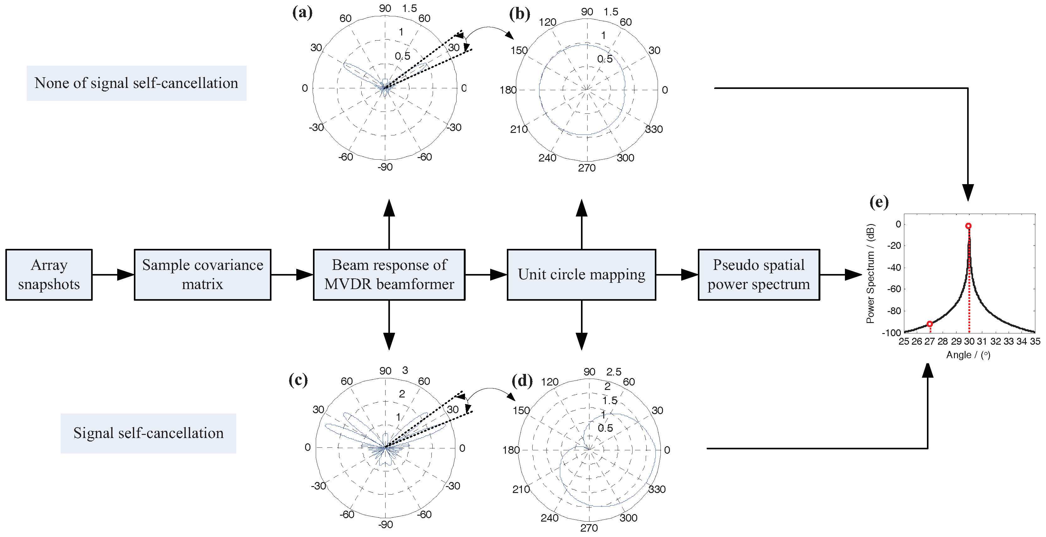
The implementation principle and detailed steps of the SSC-MVDR algorithm are shown in
Figure 1. First, the sample covariance matrix is calculated according to the array snapshots, then the beam response of the MVDR beamformer is calculated, and the beam response on the direction interval is mapped to the unit circle, and finally the pseudo spatial power spectrum is calculated. Meanwhile, in
Figure 1, examples of the beam response of the MVDR beamformer and examples of the unit circle mapping of the beam response curve segment on the direction interval are also given. Specifically,
Figure 1a,b are the results when there is no signal self-cancellation. In the
Figure 1a, the direction interval is indicated by two dashed lines, and the beam response curve segment in this direction interval is relatively flat. Therefore, in the
Figure 1b, all the mapping vector amplitudes are approximately equal. Moreover, since the phases of the mapping vectors are uniformly distributed in the range of 0 to 360 degrees, the magnitude of the sum of the mapping vectors will be very small. Therefore, the pseudo spatial power spectrum for this case will be very large, as shown by the higher red dashed line in
Figure 1e.
Figure 1c,d correspond to the case where there is signal self-cancellation. In the
Figure 1c, the direction interval is also indicated by two dashed lines, and the beam response curve segment in this direction interval contains a steep null. Therefore, in the
Figure 1d, the magnitudes of some mapping vectors are much smaller than the amplitudes of other mapping vectors. Similarly, the phases of the mapping vectors are uniformly distributed in the range of 0 to 360 degrees, thus the magnitude of the sum of the mapping vectors will be large, and the pseudo spatial power spectrum for this case will be very small, as shown by the lower red dashed line in
Figure 1e.
4. Online Computation of SSC-MVDR Algorithm
The computational complexity of an algorithm is one of the important factors we need to consider when applying the algorithm to the actual project. In the SSC-MVDR algorithm (i.e., Equation (
10)), the inverse of the sample covariance matrix and the corresponding matrix operations are the main calculation steps. In the following, the online computation process of the SSC-MVDR algorithm is given and a way to reduce the amount of calculation is provided.
First, the iterative calculation process of the sample covariance matrix is as follows
where
and
represent the sample covariance matrices at times
k and
, respectively.
is a constant less than 1 but very close to 1. When the array snapshots are non-stationary, the coefficient
is used to ensure that the SSC-MVDR algorithm still works reliably. Using the Woodbury matrix identity, the inverse of the sample covariance matrix at time
can be expressed as,
where
represents the product of the inverse of the sample covariance matrix at time
k and the array snapshot at time
, that is,
.
Second, the symbol
g is introduced to represent the generalized inner product of the steering vectors with respect to the inverse of the sample covariance matrix,
Substituting Equation (
12) into Equation (
13), the generalized inner product
g can be equivalently expressed as,
where
is defined as
Finally, the pseudo spatial power spectrum at time
can be calculated by substituting Equation (
14) into Equation (
10), that is,
It can be seen from Equation (
16) that the calculation of the pseudo spatial power spectrum at time
depends on the results of two functions, which are the generalized inner product at time
k and the function
q at time
, respectively. Please note that the former is known during the calculation process at time
(because it has been obtained in the previous calculation), and the latter is calculated as Equation (
15). Since it only involves vector operations, its computational complexity is relatively small.
5. Simulation Results and Analysis
In computer simulations, it is assumed that the linear array consists of 10 omnidirectional hydrophones, and the spacing of adjacent hydrophones is set to half the wavelength of the narrowband acoustic signal. In addition, assuming that there are two underwater acoustic sources in the far field, their directions of arrival are set to 30 degrees and 60 degrees, respectively. In the simulations below, the intensity of the acoustic source at 30 degrees is set to be variable for testing the DOA estimation performance of the SSC-MVDR algorithm, while the intensity of the acoustic source at 60 degrees is set to always be 30 dB (relative to noise) for testing the algorithm performance in a strong interference environment. Meanwhile, the received noise of the linear array is assumed to be spatially white Gaussian noise.
It should be noted that various unfavorable factors that may be encountered in the complex uncertain ocean environment are also considered in the simulations, including direction error, random wavefront fluctuations, hydrophone position errors, and hydrophone amplitude phase errors. Therefore, the steering vector model in Equation (
7) is used while assuming that the amplitude deviation coefficients of the steering vector and the phase deviation coefficients of that are known.
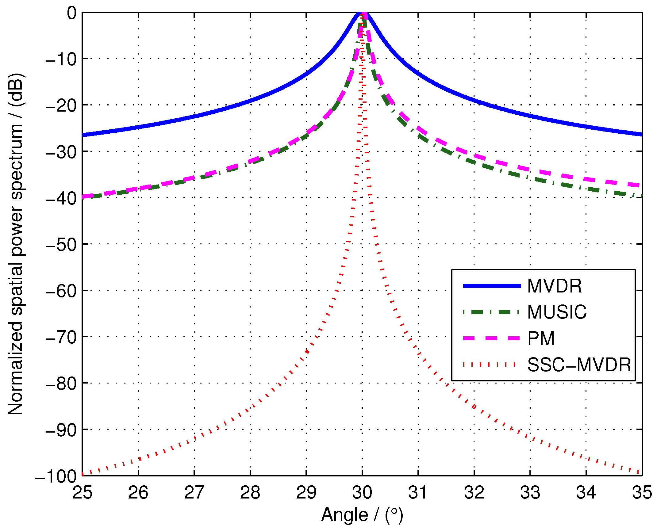
In
Figure 2 and
Figure 3, the pseudo spatial power spectrums of the SSC-MVDR algorithm are given under different acoustic source intensities and different snapshot numbers (i.e., the number of snapshots used to calculate the sample covariance matrix in Equation (
5)). Specifically,
Figure 2 corresponds to a friendly simulation environment where the signal-to-noise ratio (SNR) of the acoustic source in the direction of 30 degrees is set to 20 dB, the number of snapshots is set to 100, while
Figure 3 corresponds to a poor simulation environment where the SNR of the same acoustic source is only −10 dB, and the number of snapshots is only 30. For performance comparison, the spatial power spectrums of the MVDR method [
4], the MUSIC method [
13] and the PM method [
15] under the same simulation conditions are also given in
Figure 2 and
Figure 3. Compared to other algorithms, the SSC-MVDR algorithm exhibits sharper peaks near the true DOA of the acoustic signal in
Figure 2 and
Figure 3.
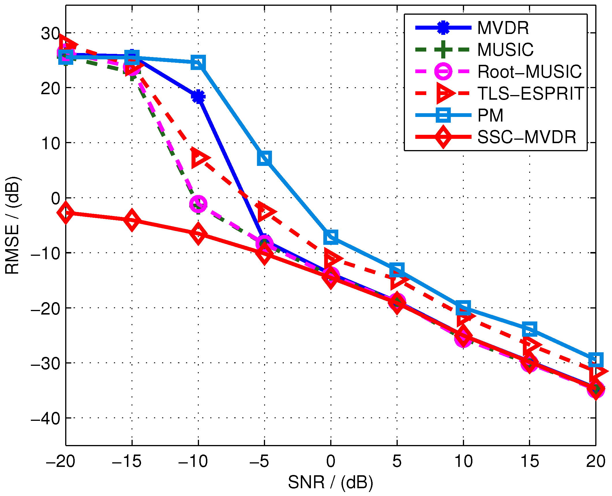
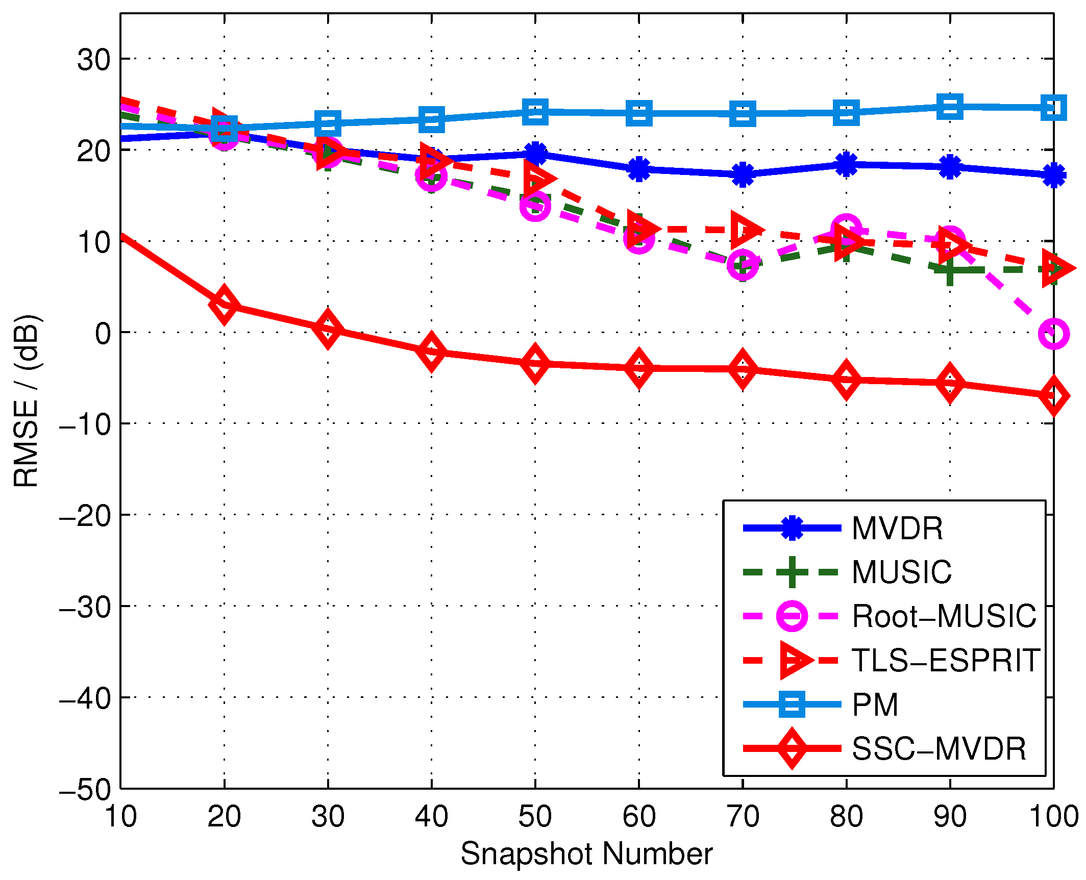
Figure 4 and
Figure 5 show the DOA estimation accuracy results of the SSC-MVDR algorithm. In
Figure 4, the number of snapshots is fixed at 100, and the intensity of the acoustic source is gradually increased from −20 dB to 20 dB. In
Figure 5, the acoustic source intensity is fixed at −10 dB, and the number of snapshots is gradually increased from 10 to 100. The DOA estimation accuracy is evaluated by the root mean square error (RMSE) of DOA estimation, which is defined as follows,
In Equation (
17), RMSE is actually the logarithm of the root mean square error, so the unit of RMSE is dB. The number of independent computer simulations is represented by
S. In the following simulations (i.e., from
Figure 4,
Figure 5,
Figure 6 and
Figure 7),
is set, which means that each simulation result requires 100 independent runs.
represents the DOA estimate obtained by the
ith computer simulation, and
is the corresponding true DOA value. Meanwhile, the results of the DOA estimation accuracy of the MVDR method [
4], the MUSIC method [
13], the Root-MUSIC method [
34], the TLS-ESPRIT method [
35] and the PM method [
15] are also given in
Figure 4 and
Figure 5. It can be seen from
Figure 4 that the RMSE results of the SSC-MVDR algorithm is significantly lower than that of other methods when the acoustic source intensity is in the range of −20 dB to −10 dB. When the number of snapshots is between 20 and 90, the RMSE results of the SSC-MVDR algorithm in
Figure 5 is also significantly lower than that of other algorithms.
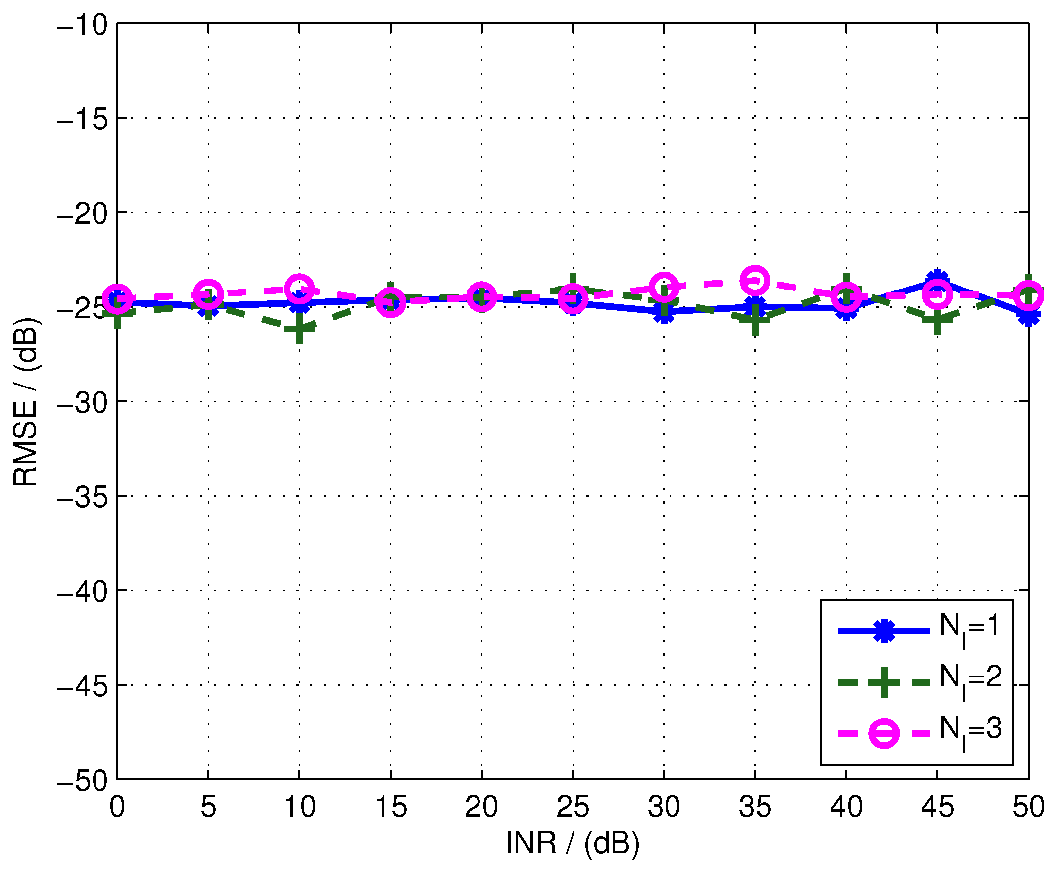
Although the interference acoustic source in the far field has been considered in the above simulation (that is, an interference acoustic source with an intensity of 30 dB and a direction of 60 degrees is always included in the simulation settings), it is still necessary to perform simulation and analysis for the case of multiple interference acoustic sources. The results of the direction estimation accuracy under multiple interference acoustic sources are shown in
Figure 6. In
Figure 6, the intensities of the multiple interference acoustic sources are set to be the same, and the interference-to-noise ratio (INR) of each interference is gradually increased from 0 dB to 50 dB. Besides,
represents the number of interference acoustic sources. For example,
means that there are 3 interference acoustic sources in the far field at the same time, their directions are 60 degrees, 10 degrees, and −20 degrees, respectively. As can be seen from
Figure 6, the three curves corresponding to different numbers of interferences are almost coincident.
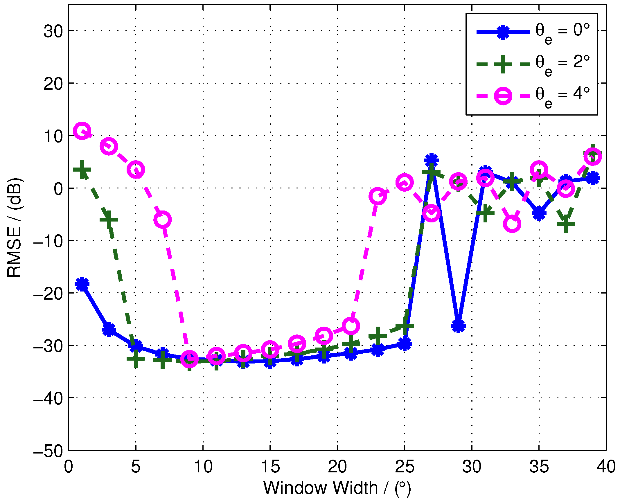
Finally, the influence of the direction interval, which is one of the important parameters of the SSC-MVDR algorithm, on the performance of the proposed algorithm is analyzed by simulation. In
Figure 7, the horizontal axis is marked as the window width, that is, the width of the direction interval
. The three curves in
Figure 7 are the accuracy results of DOA estimation obtained by the SSC-MVDR algorithm when the parameter
takes different values, where
represents the deviation of the center of the direction interval from the true DOA. It can be seen from
Figure 7 that when the width of the direction interval is in the range of 10 degrees to 20 degrees, the RMSEs obtained by the SSC-MVDR algorithm is significantly lower than that when different window widths out of the above range is used. The reason for the above results is that when the center of the direction interval deviates from the true DOA and the selected direction interval is too narrow, the actual DOA of the acoustic source will fall outside the selected direction interval, thus the obtained DOA estimation must be wrong. However, when the selected direction interval is too wide, it will cause the beam response segment in the direction interval to contain some unwanted or even unfavorable information, such as other nulls in the beam response that are independent of signal self-cancellation.


