Numerical Modelling of the Fire Extinguishing Gas Retention in Small Compartments

Featured Application

Featured Application: The numerical modelling approach presented here may be useful for the design of fixed gaseous extinguishing systems in various compartments, with the emphasis of process safety (3D printing, server rooms, clean industrial facilities), as well as energy generation (turbine halls, wind turbines, etc.) and storage. The presented mixtures of fire extinguishing gases with a density close to air provide significantly longer protection times, compared to the mixtures used today, which can be used to increase the fire safety of facilities with limited accessibility. The Computational Fluid Dynamics (CFD) model, coupled with the leakage test, can be used to choose the proper mixture for the given compartment, and in the near future possibly as a tool for real-time decision making.

Abstract

Active fire protection systems are critical elements of good process safety. Among them, gaseous extinguishing systems provide quick, clean suppression and prolonged protection due to long retention process of the gas. Standard design methods do not provide sufficient tools for optimisation of the retention process, thus the necessity for development and validation of new tools and methods—such as Computational Fluid Dynamics (CFD) simulations. This paper presents a simplified approach to CFD modelling, by the omission of the discharge phase of the gas system. As the flow field after discharge is stable and driven mainly by the hydrostatic pressure difference, buoyancy and diffusion, this simplified approach appears as an efficient and cost-effective approach. This hypothesis was tested through performing CFD simulations, and their comparison against experimental measurements in a bench scale in a small compartment (0.72 m³), for six mixtures that differ in their density. Modelling the retention of the standard IG55 mixture was very close to the experiment. Modelling of mixtures with a density close to the density of ambient air has proven to be a challenge. However, the obtained results had sufficient accuracy (in most cases relative error <10%). This study shows the viability of the simplified approach in modelling the retention process, and indicates additional benefits of the numerical analyses in the determination of the fire safety of protected premises.

1. Introduction

1.1. Fire Protection in Industrial Safety

Fire protection systems help mitigate the effects of a fire in industrial facilities. Fire protection was declared an “underpinning of good process safety” by [1] and was separated into two distinct branches: passive and active systems. This simple classification of fire safety systems is the base of most of the fire safety regulations, not only in the process industry but also in the whole of civil engineering [2]. In some aspects, the classification of systems into passive and active solution also reassembles the segregation used for explosion and detonation prevention and suppression [3]. In fire safety, passive systems act by limiting the growth of the fire, confining the fire within a compartment and improving the structural resistance to fire. The active systems typically act by early detection or suppression of the fire. In the case of suppression, [1] focused mainly on traditional water-based fire extinguishing systems such as sprinkler systems. However, it must be noted that besides sprinkler systems, modern fire safety engineering includes a vast array of water-based suppression technologies, such as high-pressure water mist suppression systems [4,5], high expansion foam systems [6] or water spray curtains used to mitigate hazards related to toxic gases [7,8]. Despite their well-known performance, in some areas of the modern industry, the release of water from water-based fire extinguishing systems can cause unacceptable losses. Examples of such areas are trafo-stations and power supply rooms, turbine halls, server rooms, laboratories, 3D printing and CNC facilities, etc. In some cases, water-based systems may also have a negative impact on the structure [9,10]. In these spaces, different suppression techniques must be employed, among them: fixed gaseous extinguishing systems (further referred to as FES-gaseous) [11], powder extinguishing systems [12] or inertisation [13,14]. An emerging area where gaseous systems may find suitable use is in energy storage facilities, primarily based on Lithium batteries that pose significant fire hazard [15,16,17]. Also, the use of gaseous systems is promoted in some compartments, where the release of water-based medium may cause problems with visibility in smoke. Besides limiting losses related to the occurrence of the fire, some remote facilities require an additional layer of protection by prolonged suppression effect of the used medium. In such a case, the FES-gaseous systems optimised for prolonged retention time are highly feasible [11].

1.2. Use of Gaseous Fire Extinguishing Systems

FES-gaseous systems operate by filling the protected space with fire-extinguishing gas, stored under pressure in reserve (cylinders), connected with a pipeline ending with nozzles. The gas outflow is automatic, once the fire detectors detect a fire. The outlet nozzles are selected and arranged to ensure uniform distribution of the fire-extinguishing gas in the whole protected space. FES-gaseous systems tend to be used to reduce the risk of property loss and fire spreading around the facility, but they are also regarded as an essential solution from the safety of humans, rescue teams and building [11].

Before the gas discharge (Figure 1A), the flow field in the compartment is dominated by the turbulent motion created by buoyant smoke plume and flames. During discharge (Figure 1B) the flame is quenched, and any earlier flow-field overpowered by highly turbulent, supersonic gas discharge. At the end of the discharge phase, the pressure inside and outside of the compartment is evened out by a pressure relief damper, and the resulting gas concentration is uniform in the space. After the discharge (Figure 1C), the flow inside the compartment settles down, and the concentration of gas is uniform and should be equal to the designed concentration. The turbulent gas exchange takes place at the leakages, and near heat sources, ventilation elements. Stage (Figure 1C) is taken as the initial conditions for simulations in this paper. The extinguishing gas concentration (and the Oxygen concentration as a result) during, and immediately after, the discharge is variable in the compartment volume. However, as observed during the experiment [11], these concentrations level out in a short time after the discharge in the whole protected volume. Further to that, in the standardized approach (described further in Section 1.3) the “retention time” is measured not from the discharge, but from the moment when Oxygen concentration in the compartment reaches the design value. Thus, taking into account the complexity of discharge modelling, the simplification of the CFD approach to initialize the simulation with the “design conditions” and not the discharge seem justified.

Successful firefighting with fire-extinguishing gas entails the need to maintain the designed fire-extinguishing gas concentration in the protected space for the required period, which is called the retention time. It stands for the time necessary to suppress the flame and take actions by appropriately trained staff. A longer retention time increases the probability of effective rescue operations and extinguishing the fire in its initial phase. Consequently, the longer the retention time, the higher the fire safety, while too short retention time may result in the fire recurrence and spreading. The retention-time optimisation method, by altering the FES-gaseous mixture density, was presented and described in depth in [11].

In this paper, we attempt to model the FES-gaseous retention process with the use of a Computational Fluid Dynamics (CFD) model—ANSYS^® Fluent^® (version 14.5.0 [18])—based on the previously published experimental study [11,19]. Significant simplifications in the initial conditions of the simulation were introduced to limit the complexity of numerical modelling of FES-gaseous protection. It was observed in the bench-scale experiments [11] that after initial gas discharge, the compartment is uniformly filled with the gas, and there were no significant differences in the gas concentration in space. This is mainly due to pressure relief mechanisms used in protected areas, that act as a fail-safe to reduce the damage caused by the gas release. Modelling the super-sonic discharge through a minuscule nozzle along with the pressure relief mechanism could be considered as a significant challenge. Besides the technical challenges, the explicit modelling of release and pressure relief would require substantially larger amount of computational resources, due to much smaller space- and time-scales that have to be resolved. Thus, as mentioned previously, we chose to omit this phenomenon and initialise the simulations with the design concentration of the extinguishing gas and stabilised flow field within the protected compartment, Figure 1C. Verification of the hypothesis that omission of the discharge modelling will not cause significant error in the prediction of the retention time, and the gas flow in and out of the protected premise is the primary goal of this paper. As the work bases on the previous experimental study [11], the simulations were performed for a compartment that can be considered representative of a control panel, server cabinet or similar smaller electronic equipment.

1.3. Limitations of Standardised Models

For optimum fire safety level of premises protected by FES-gaseous systems, it is vital to select the right quality and quantity of the fire-extinguishing gas, which will extinguish the fire immediately after being released to space and will prevent fire recurrence. The fire-fighting process effectiveness depends on some factors, including the fire-extinguishing gas retention in the premises [20]. The time is usually identified analytically, according to selected models of the gas flow from the premises. A review of current standards concerning FES-gaseous systems is given in work [11,21], where we identified the following analytical models:

• Model with a sharp interface between extinguishing gas and air, presented in NFPA2001 [22];
• Model with wide interface between the gas and air, presented in EN15004 and ISO14520-1 [23,24];
• Model of continuous mixing of extinguishing gas with air, at a constant rate within the volume—valid for areas in which the air is continuously moving, e.g., through air-conditioners [22,23,24].

Verification of the applied models suggests discrepancies between the measured and identified values [25]. The assumptions for the applied models do not work for gases whose density is similar to the density of air, under specific environmental conditions. Standard models assume a different profile of the fire-extinguishing gas distribution in a room (gas stratification) than for gases with a density similar to the density of air (natural gas mixing). Moreover, standard models do not take into consideration the impact of atmospheric conditions on the value of air density inside and outside the protected premise, as well as on the fire-extinguishing gas density. The acquired parameter values are identified for normal conditions. Standard models assume a constant and equal value of the pressure inside and outside the protected space. Another limitation observed for standard models is a lack of possibility to cover the impact of phenomena occurring alongside with the gas outflow from the cylinders or gas flow through the room (turbulence, temperature drop, different physical form) and not covering the impact of internal sources of heat, including the impact of fire. Another simplification in standard models is neglecting or simplifying the architectural characteristics of the room (equipment inside, the shape of the compartment, the presence of architectural barriers, etc.). Finally, standard models do not fully account for the impact of the sources of flow inside the protected space—protected machinery, fans, air-conditioners, etc. The devices cause a turbulent movement, which can disturb the natural flow after the gas has been discharged.

2. Materials and Methods

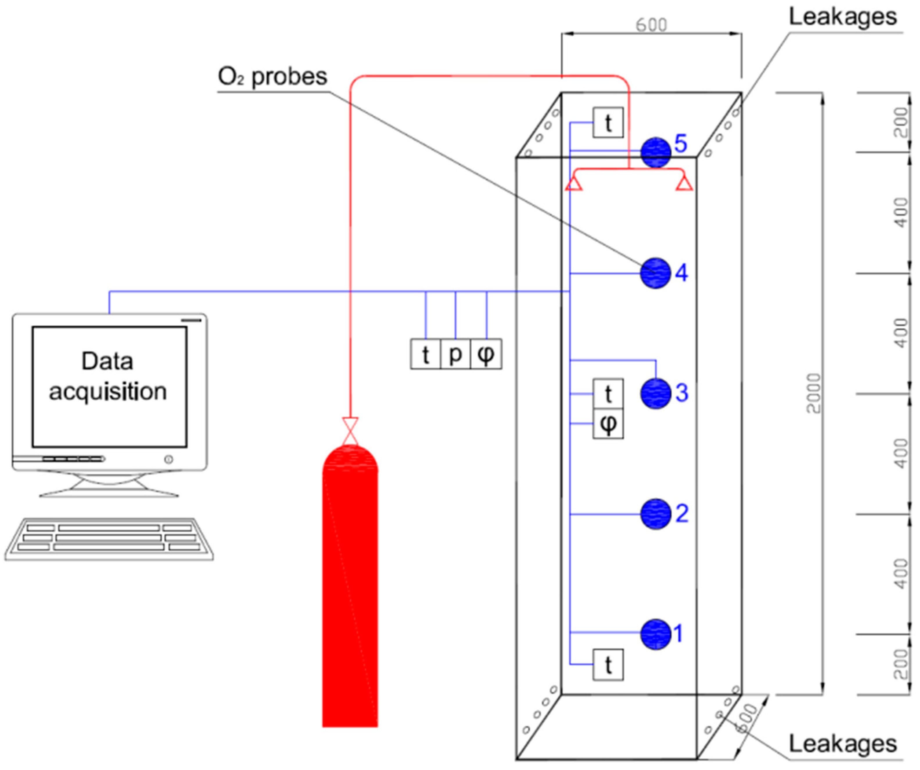
2.1. Experimental Study on Extinguishing Gas Retention Time

An experimental investigation was performed [11] in order to maximise the retention time by choosing a gas mixture, whose density is close to the density of ambient air. During these experiments, a total number of 41 discharges for 8 different mixtures were performed. The primary measurements were the measurement of oxygen concentration and air/gas temperature and humidity. The flows were not measured, as they were not crucial for the primary goal of the experiment. The test rig was placed inside a chamber with climate control, which allowed controlling the external ambient conditions.

The test rig reassembled small server type cabinet and is representative for local protection of process equipment. However, this can also be considered as the most unfavourable conditions, due to high leakage to floor area/volume ratio, as well as the chosen placement of the leakage openings. Due to this, the chosen test array may be considered partially representative to large compartment geometry [11], although further verification in a larger geometrical scale is necessary. The test rig had dimensions of 0.6 m × 0.6 m × 2.0 m, and the volume of 0.72 m³, Figure 2. The leakages were modelled by drilled openings (eight located in the bottom, and eight located on the top), with a total area of 18 cm². Based on the previous design experience in commercial projects, the design concentrations of extinguishing gases in the test rig was chosen as 45%, which corresponds to the oxygen concentration of 11.5%. Measurements of the oxygen concentration were carried at heights of 0.20 m, 0.60 m, 1.00 m, 1.40 m and 1.80 m above the rig floor, and performed with an electrochemical sensor with a range of 0–25% V/V ± 0.1% V/V.

The detailed description of the experiment and its results are presented in [11].

The results of this experimental program were chosen as the reference for the numerical analyses presented in this paper. Due to the limitations of the experimental measurements, the authors did focus on a comparison of oxygen concentrations at five measurement points, which are the indication of the local extinguishing gas concentration. As in the further numerical modelling the gas discharge was omitted on purpose, it was critical to defining the criteria for time synchronisation between experiment and simulation. Authors arbitrarily chose that the t = 0 s in the simulation will refer to the instance in the experiment when the measured oxygen concentration at all of the measurement points reached 11.5%. This corresponds to the initialisation of the CFD simulation with a uniform gas concentration of 45% (oxygen concentration of 11.5%) in the protected compartment.

2.2. Numerical Modelling of Gaseous Fire-Extinguishing Systems

Numerical representation of gaseous fire-extinguishing system operation with Computational Fluid Dynamics (CFD) models could be used for the design of better gas-mixtures, optimisation of shape and sizes of protected compartments, or to improve the location of nozzles. However, in the current state of the art, such modelling is not a trivial task. Following some of the best practice guidelines for CFD [26], steady-state RANS (Reynolds-Averaged Navier–Stokes) modelling of stratified gas mixtures for higher Rayleigh numbers shows deficiencies, as classical turbulence models use an isotropic approach for Reynolds stresses and Boussinesq approximation for the density-temperature dependency. Also based on [19], modelling of fire-extinguishing gas flow through minor gaps makes a great challenge for the existing mathematical models. The guidelines [26] recommend possible solutions for the modelling of such complex phenomena, which are the use of URANS (Unsteady RANS model used in this study), Reynolds Stress or Large Eddy Simulation models.

The buoyancy of the layers must be resolved [26], as well as the mixing and diffusion in the intermediate layer. In the case of gas mixtures, which have a difference of density between gas and ambient air close to 0 (Δρ → 0), the buoyancy has a minor effect, and diffusion and turbulent mixing may be the most important phenomena. The buoyancy will also dive the flow through the leakages, where turbulent mixing of air and gas will occur. To accurately model the flows in the leakages, the minuscule details of the leakages had to be resolved explicitly, which means that the prepared numerical model had a significant difference of scales between the large details (e.g., compartment architecture) and the small details (e.g., nozzles, leakages).

The flow of extinguishing gas inside and outside of protected compartment may be driven by following physical phenomena and interactions, which were included in our considerations:

-

Difference of buoyancy between gas and air, and the phenomena that take part at the interface of the buoyant layer (e.g., diffusion, turbulent mixing);

-

Flow of clean air into to the protected compartment through leakages;

-

Flow of extinguishing gas out of the protected compartment through leakages;

-

The temperature gradient in and out of the protected compartment.

Other significant phenomena and interactions that can possibly influence the retention of the extinguishing gas beyond the scope of this paper are, among others:

-

Forced ventilation inside of the protected compartment;

-

The non-uniform release of the gas and the use of local pressure relief dampers;

-

Heat sources in the compartment (e.g., server heat sinks);

-

Pressure gradient outside of the chamber (e.g., due to wind effects);

-

The source of fire itself.

2.3. General Description of the CFD Method

Numerical fluid flow simulation involves solving systems of differential equations describing the analysed phenomena. Basic equations solved for all tasks are the equations describing the velocity and pressure field (continuity equation) and Navier–Stokes movement equations. For calculations of the smoke and heat spread, additional equations of energy and radiation conservation and smoke transport are solved. The description of the CFD method used in fire safety engineering was presented by McGrattan [27] and Merci [28]. Theoretical foundations of the CFD method are described [29,30,31]. The set of equations presented by McGrattan is the same, as the mathematical model of ANSYS Fluent software [18] used by the Authors in the experiments presented in the paper.

In the context of this paper, the mass conservation Equation (1) of the CFD model means that the fire-extinguishing gas can be removed from the model only when it flows out through the domain boundary. The density change in any volume equals the mass flow through its boundaries (leakages) or the mass introduced through the source in the volume (${\dot{m}}_i^{‴}$), which in this case is equal to 0.

$$\frac{\partial \rho }{\partial t}+\nabla ·\rho \overrightarrow{u}={\dot{m}}_i^{‴}$$

(1)

where: ρ—density, t—time and u—velocity.

The extinguishing gas within the air-gas mixture is modelled as a single mixture ingredient (Y_gas), and its transport can describe by the Equation (2).

$$\frac{\partial (\rho Y_i)}{\partial t}+\nabla ·(\rho Y_i\overrightarrow{u})=\nabla ·\left(\rho D_i\nabla Y_i\right)+{\dot{m}}_i^{‴}$$

(2)

where: D_i is the dispersion coefficient of i-th species.

The momentum conservation Equation (3) is expressing the preservation of the Newton’s Second Law of Motion. The forces causing the fluid flow are composed of the pressure field $\nabla p$, tension (tensor $\overline{\overline{\tau }}$), buoyant force $\rho \overrightarrow{g}$ and external forces $\overrightarrow{F}$, which in this case are equal to 0, (3).

$$\frac{\partial (\rho \overrightarrow{u})}{\partial t}+\nabla ·(\rho \overrightarrow{u}\overrightarrow{u})=-\nabla p+\nabla ·(\overline{\overline{\tau }})+\rho \overrightarrow{g}+\overrightarrow{F}$$

(3)

Since the tests performed took into account the difference in the temperature inside and outside the test chamber, as well as the temperature gradient outside the chamber, the heat flow in the system was modelled using the energy conservation Equation (4), which identifies that the enthalpy (5) in any point changes according to the stream of energy flowing into the control volume. The equation also considers the possibility of heat generation directly in the finite element (${\dot{q}}^{‴}$), which in this case amounts to 0. Heat can also be delivered as a result of the fluid kinetic energy dissipation as a result of friction ($\epsilon$), the impact of pressure ($\frac{Dp}{Dt}$) or heat radiation. In fire-safety related applications, the term responsible for the pressure field impact or kinematic energy dissipation is usually neglected.

$$\frac{\partial (\rho h)}{\partial t}+\nabla ·(\rho h\overrightarrow{u})=\frac{Dp}{Dt}+{\dot{q}}^{‴}-\nabla ·\overrightarrow{q}+\epsilon$$

(4)

$$h={\displaystyle \underset{T_0}{\overset{T}{\int }}{c}_{p}dT}$$

(5)

A change in the density can be sufficiently described by a perfect gas Equation (6). M_avg (7) in Equation (6) stands for the averaged molecular weight of the gas mixture ingredients, whose concentration can be identified in any volume using (2).

$$p=\frac{\rho \Re T}{M_{avg}}$$

(6)

$$M_{avg}=\frac{1}{{\displaystyle \sum \frac{Y_i}{M_i}}}$$

(7)

where: p—pressure, $\Re$—gas constant, T—temperature, Y_i—vol. concentration of i-th species, M_i—molar mass of the i-th species.

The initial weight of the fire-fighting gas in the chamber was modelled by identifying the mean molecular weight for the selected gas mixture, assuming a perfect homogeneity of the mixture, and then providing the mixture with a specific temperature and initial pressure.

Some notable examples of practical use of CFD method in fire safety engineering are presented in [32,33,34]. CFD method was also widely used to investigate gas dispersion in process safety. Most of the recent works relate to the release of heavy gasses [35,36,37,38] or light gasses [39,40], while the focal point of this paper is on the mixtures with a density very close to the density of ambient air.

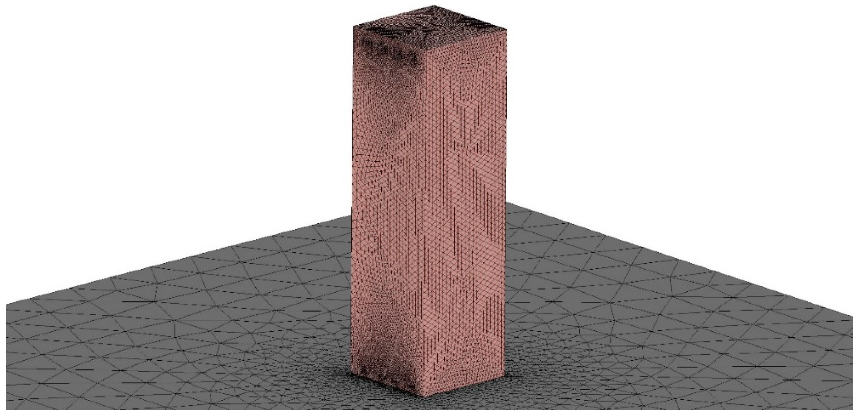
2.4. Numerical Model—Assumptions

Numerical tests of gas flow were carried out in a closed array, based on the experiment described in Section 2.2 and [11]. A numerical representation of the test rig was developed, following the dimensions shown in Figure 2. The leakages were introduced as physical holes in the skin (modelled explicitly, as they were in the experiment). Numerical tests were conducted following assumptions analogical to the relevant experimental data presented in the paper [11]. The numerical model took into consideration the diversified conditions of the environment outside and inside the measurement chamber, which greatly determined the density of air and fire-extinguishing gases taken for the calculations. The fire-extinguishing gas discharge from the cylinders was not modelled explicitly, nor was the fire within the protected premises, and the impact of the simplifications are discussed in Section 3 and Section 4. The calculations were initiated assuming a uniform concentration of the fire-extinguishing gas in the whole chamber volume. In most cases, the assumed fire-extinguishing gas concentration amounted to 45%, which corresponds to 11.5% oxygen concentration (v/v) in the chamber (

Table 1. List of initial conditions taken for modelling.

No.	Ar [%v/v]	N2 [%v/v]	Δρ = dm − d0 [kg/m3]	Gas Molar Mass M	Volume Fraction Oxygen	Volume Fraction Gas	Temp. (out.) [K]	Temp. (ins.) [K]	p [hPa]
1	50	50	0.192	33.557	0.115	0.45	289.75	288.45	1003
2	0	100	−0.039	28.013	0.115	0.45	288.75	289.25	1003
3	10	90	0.007	29.122	0.105	0.50	293.15	29415	1010
4	6.9	93.1	−0.007	28.778	0.115	0.45	290.25	291.55	1002
5	7.8	92.2	−0.003	28.878	0.113	0.46	292.65	292.05	1008
6	7.5	92.5	−0.004	28.845	0.115	0.45	292.85	294.35	995

). One should note here that the retention time is defined as the time from starting the analysis to reaching oxygen concentration of 13% at any measurement point.

The modelling took into account the presence of temperature gradient outside the measurement for better representation of the reference experiment. A constant value of temperature after discharge and mixing of gases in the chamber was assumed, according to the experimental data (Figure 3; Figure 4).

Time discretisation was performed with a fixed discrete time step of 0.5 s, and the convergence criteria were analysed: 10⁻³ for continuity, mass transport, the kinetic energy of turbulence (k) and the dissipation of the kinetic energy of turbulence (ε), and 10⁻⁶ for the conservation of energy. For the Large Eddy Simulation (LES) solver, the time step was shortened to obtain the convergence. The SIMPLE numerical scheme was chosen for pressure-velocity coupling. Spatial discretisation was performed with second-order upwind schemes, except the momentum equation for the LES model, in the case of which the bounded-central differencing method was used. The gradient was calculated using Green–Gauss theorem, based on node values.

The exterior domain was closed with third-type wall boundary conditions (external domain was sealed). However, the volume of the domain was 103 times larger than the internal chamber. The chamber was modelled with thin (3 mm) wall elements, and the material was steel (ρ = 7800 kg/m³, λ = 40 W/m·K). The temperature inside and outside of the chamber was set in accordance with measurements from full-scale experiment. Leakages were modelled as interior-type face elements.

The numerical modelling was performed for 6 scenarios, as shown in Table 1.

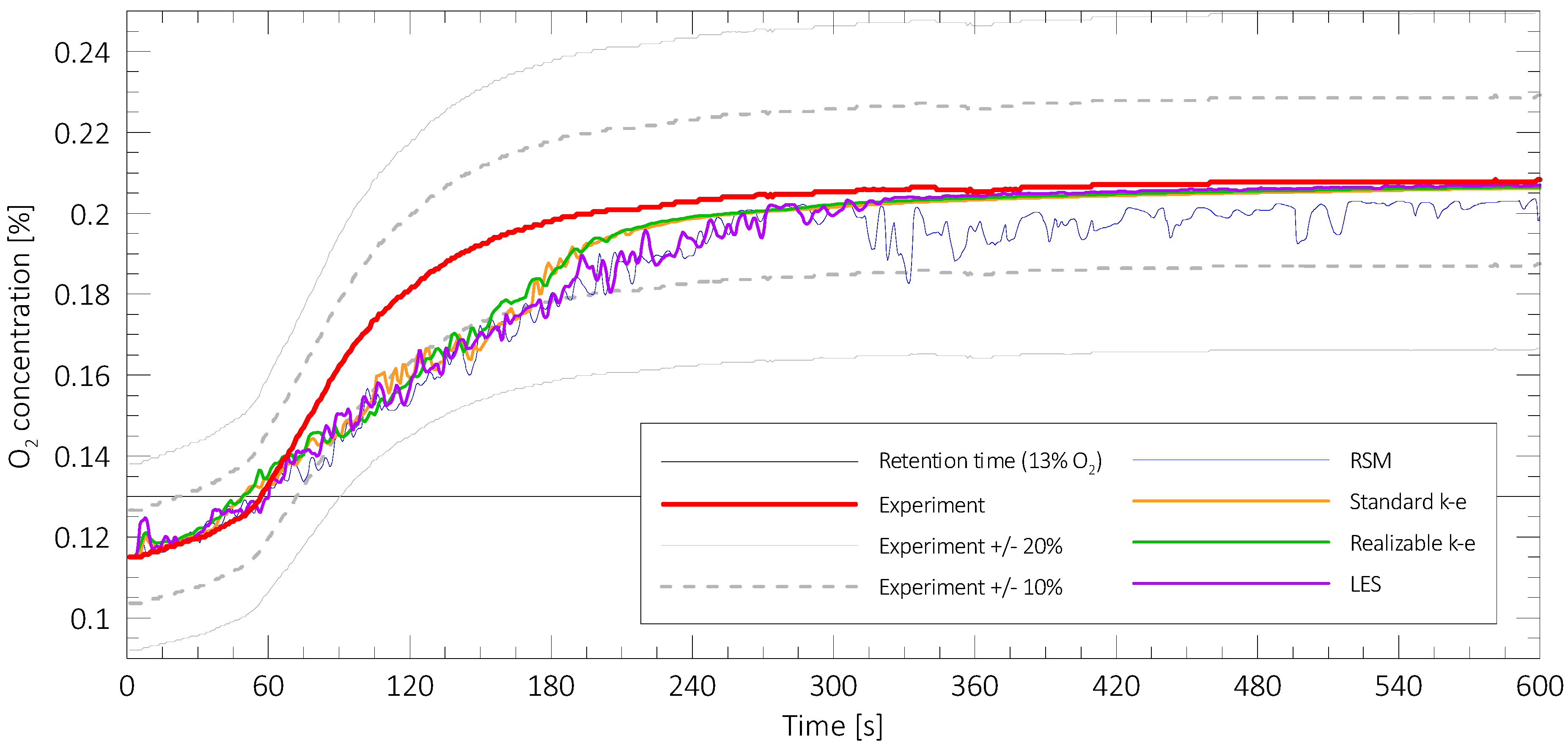
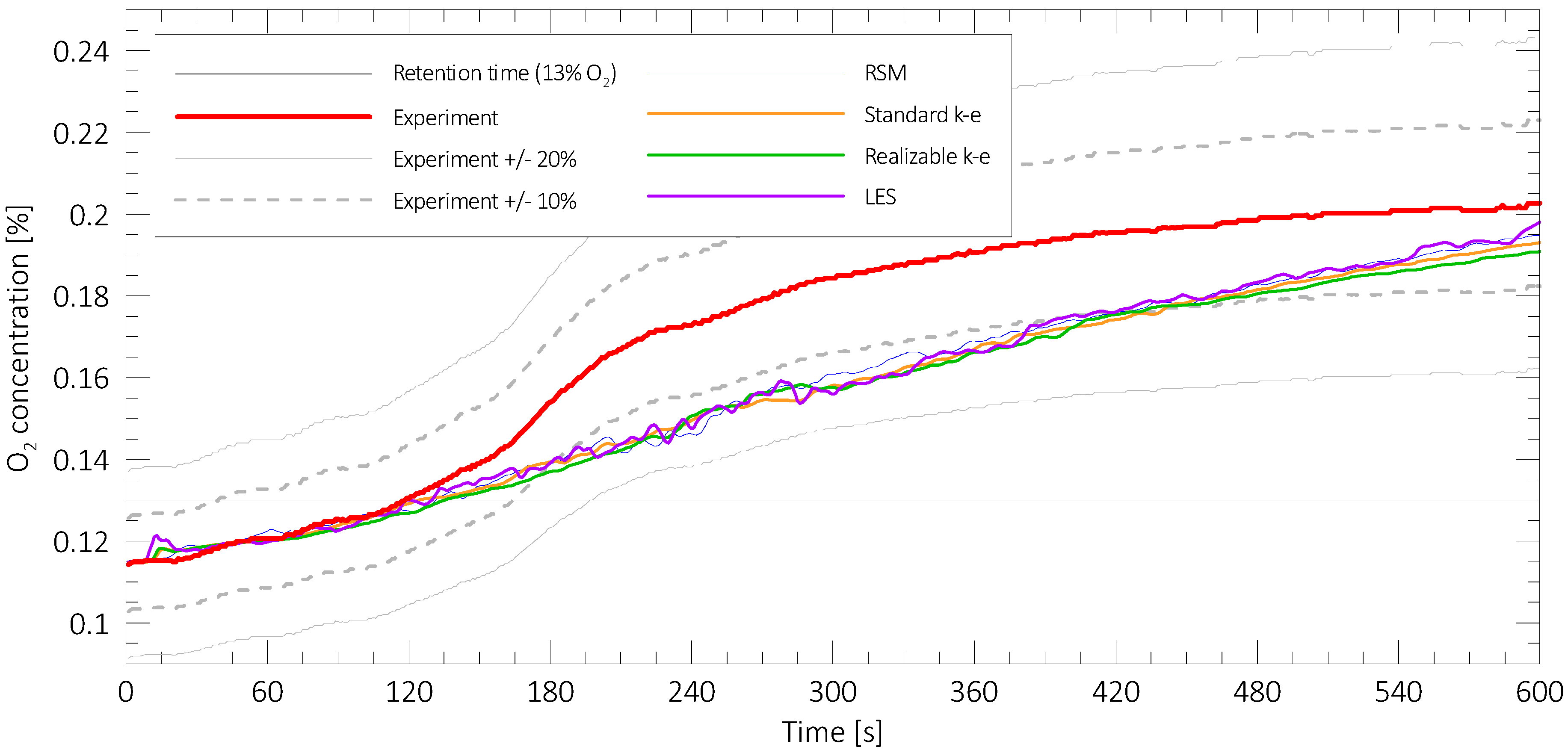
2.5. Turbulent Flow Sub-Model Sensitivity Study

The issues solved within the analysis of smoke and heat spreading are often highly turbulent, and, consequently, the description of the velocity and pressure field has a complicated form. The mainstream turbulence models include Reynolds-Averaged Navier–Stokes (RANS) for an in multiple variants (RANS k-ε, RANS k-ω, RSM and others), Large Eddy Simulation (LES) and hybrid models. RANS method solved for sequential time steps in order to capture transient phenomena is referred to as Unsteady RANS (URANS). An in-depth review of the RANS and LES turbulence models was recently published by Blocken [41]. Although the flows in fire environment are usually turbulent, it is not necessarily the case in compartments post-discharge of a FES-gaseous system. Dependant on the hydrostatic pressure, the flow into and out of protected compartment may be turbulent or laminar, and the phenomena inside of the protected compartment may be driven mainly by diffusion and buoyancy.

Nevertheless, for practical use of the method in ventilated compartments, and in case of fire, the turbulence model will be among the most important sub-models. As a direct discrete solution to Navier–Stokes equations is not possible in a large scale (with a reasonable amount of resources), following four approaches to turbulence modelling were investigated: URANS standard k-ε, URANS Realizable k-ε, Reynolds Stress Model (RSM) and Large Eddy Simulation (LES).

RANS method applies a time-averaged solution of N-S equations, with the additional decomposition of velocity, pressure and field function into the averaged component and the fluctuation. In order to close the model, the Boussinesq hypothesis is applied, which relates the viscous friction and turbulent Reynolds stress. The total turbulent energy consists of following elements, which eventually lead to the formation of the kinetic energy term (k, 8), and the dissipation rate of the kinetic turbulence energy (ε, 9):

$$k=\frac{1}{2}{\displaystyle \sum }_{i=1}^3(\overline{{v^{\prime }}_i^2})$$

(8)

$$\epsilon =(2{\mu }_t/\rho )\overline{)s_{ij}^{\prime }{s}_{ii}^{\prime }}$$

(9)

where: ν—kinetic viscosity, ρ—density, s—Reynolds stress.

The turbulent viscosity term μ_t is determined using the following relation (2.10):

$${\mu }_t=C\rho \nu l=\rho C_{\mu }\frac{k^2}{\epsilon }$$

(10)

The constants of “standard” RANS k-ε are: C_µ = 0.09; σ_k = 1.00; σ_z = 1.30; C_1z = 1.44; C_2z = 1.92.

In realizable k-ε the turbulent viscosity is described in an elaborate form and forms a new equation that describes the dissipation rate of the kinetic turbulence energy, ε. The Reynolds stress is calculated as incompressible strained mean, by combining the Boussinesq relationship and the eddy viscosity definition [18].

In the Realizable k-e model the C_μ is no longer a constant, but a function of the mean strain and rotation rates, the angular velocity of the system rotation and the turbulence fields. It can be computed from Equation (11), with use of additional model constants A₀ and A_s:

$$C_{\mu }=\frac{1}{A_0+A_s\frac{k{U}^{*}}{\epsilon }}$$

(11)

U* is computed with the inclusion of not only strains but also rate of rotation tensor, in frame with the angular velocity. The complete explanation of calculation procedure may be found in [18]. The model constants are: C_1ε = 1.44; C₂ = 1.9; σ_k = 1.00; σ_ε = 1.20.

The third RANS approach used in this work—the Reynolds stress equation model (RSM)—is often referred as second moment closure [42,43]. It can be considered as much more elaborative traditional model, than previously described k-ε approach. In RSM model the hypothesis of isotropic eddy-viscosity is abandoned, and the N–S equations are solved for the Reynolds stresses, together with an equation for the dissipation rate. This means that in three-dimensional space, this model requires seven additional transport equations, which account for the streamline curvature, swirl, rotation and rapid changes in strain rate. Due to the nature of the model and the amount of additional equations, this model can be considered computationally expensive, in comparison with k-ε modelling. The buoyancy is included in the model as a force (G_ij). This model assumes that the value of turbulent Prandtl number is 0.85 [18].

Another popular approach to turbulence modelling in fire safety is so called Large Eddy Simulation (LES) [44]. In this model large eddies of the flow are resolved directly, while small eddies are modelled. The assumption is that small eddies are less dependent on the geometry, tend to be more isotropic—thus may be simulated in a more universal way. The large eddies are usually problem dependent, and since they cannot be modelled universally, they are resolved directly. The boundary between large and small eddies is referred to as the Smagorinsky filter, and typically is the size of the discrete element. Since it is not possible to directly model eddies smaller than the size of the mesh, the solution is more dependent on the grid quality. More to that, in order to properly resolve the flow field the Courant–Friedrichs–Lewy criterion should be satisfied (CFL < 1), which leads to significant requirements towards the time-scale resolution of the simulation. For a successful use of LES model, it can be assumed that not less than 80% of the energy is resolved [45]. The filter size is applied to the governing equations (especially the N–S equations), while rest of the flow is resolved with a sub-grid model. In the case of this study, LES model was used only for comparison, and as such will not be discussed in details, which may be found in [27,44].

For the purpose of the choice of the turbulence sub-model, a sensitivity analysis consisting of 8 simulations was performed. Two mixtures were chosen for this study (No. 1 and 2, Table 1). The following turbulent flow submodels were used: (a) standard k-ε, (b) Realizable k-ε, (c) Reynolds stress model (RSM) and (d) LES. The sensitivity study focused on the oxygen concentration at the probe, for which the retention time was reached the soonest. For both of the tested mixtures, no major differences were found with the use of different turbulent flow submodels, Figure 5 and Figure 6. The minor discrepancy was found for the RSM model in scenario No. 1, in which oscillatory behaviour was observed. However, the predicted retention time with this model was close to one measured in the experiment. As no major influence of the turbulent flow sub model was found, the most economical sub-model (Realizable k-ε) was chosen for the remainder of this study.

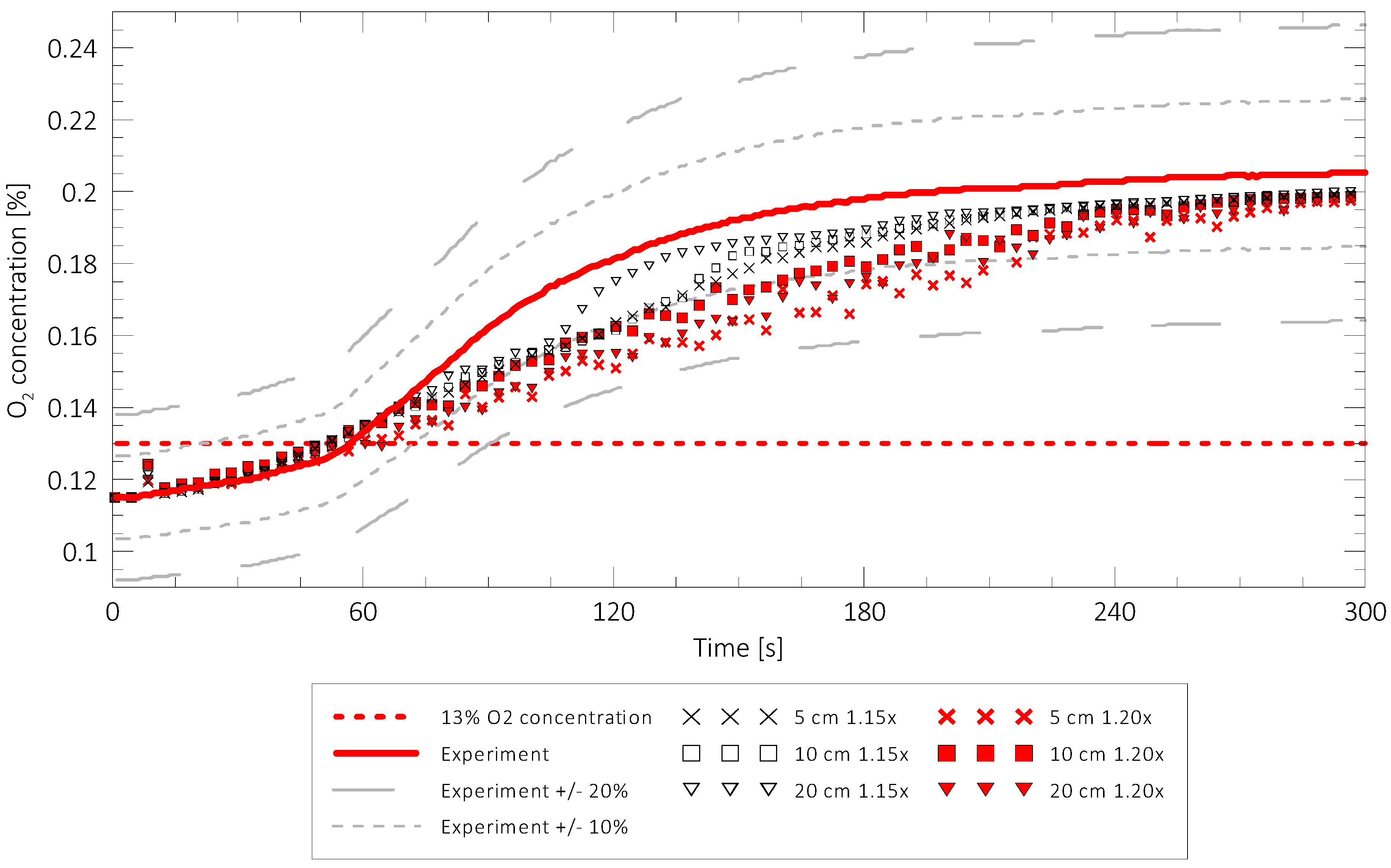
2.6. Mesh Sensitivity Study

The numerical mesh quality may have significant impact on the results of numerical calculations, thus a mesh sensitivity study is required to support the choice of numerical mesh [46]. In case of this study, the numerical domain was discretised in space using a non-structural tetrahedral mesh. The final mesh was chosen after a series of numerical analyses, in which the mesh was refined until no further change in the results of numerical was observed.

The mesh was densified near the upper and lower leak holes, where intensive flow phenomena could be expected. The mesh size at the leakage was set as 5 mm (a smaller mesh of 2 mm was also investigated). The interior of the test chamber meshed with three different element sizes—50 mm, 100 mm and 200 mm. The intermediate mesh size between the smallest and the largest elements is determined by the mesh growth function, which is the relative difference in size between neighbouring elements. For this project, two mesh growth functions were investigated—1.15 and 1.20. However, it must be noted some best practice guidelines recommend values up to 1.3 [26]. The study was performed for Scenario No. 1 (50% Ar 50% N₂ gas mixture), with RANS k-ε Realizable solver, and consisted of 6 numerical simulations.

The results are presented in Figure 7. The mesh with larger growth rate function (filled symbols) yielded lower gas concentrations, which means it underestimated mixing. For a mesh with 1.15× growth rate, minuscule differences were noticed. Additional improvement in the mesh by changing the mesh size at the leakage to 2 mm at the leakage did not significantly alter the results. Balancing the solution quality and the computational cost, the final mesh chosen for numerical experiments had the size of 5 mm at the leakages and 50 mm in the domain, with a 1.15 growth rate function. For this function, the expected results of gas concentration were in a 10% range from the experimental measurements, for gas mixture No. 1.

The mesh size for the surrounding domain was chosen as 300 mm with a 1.15 mesh growth function. The coarser mesh was chosen for the exterior, as no relevant parameters were measured in this space. An overview of the mesh is shown in Figure 8.

3. Results

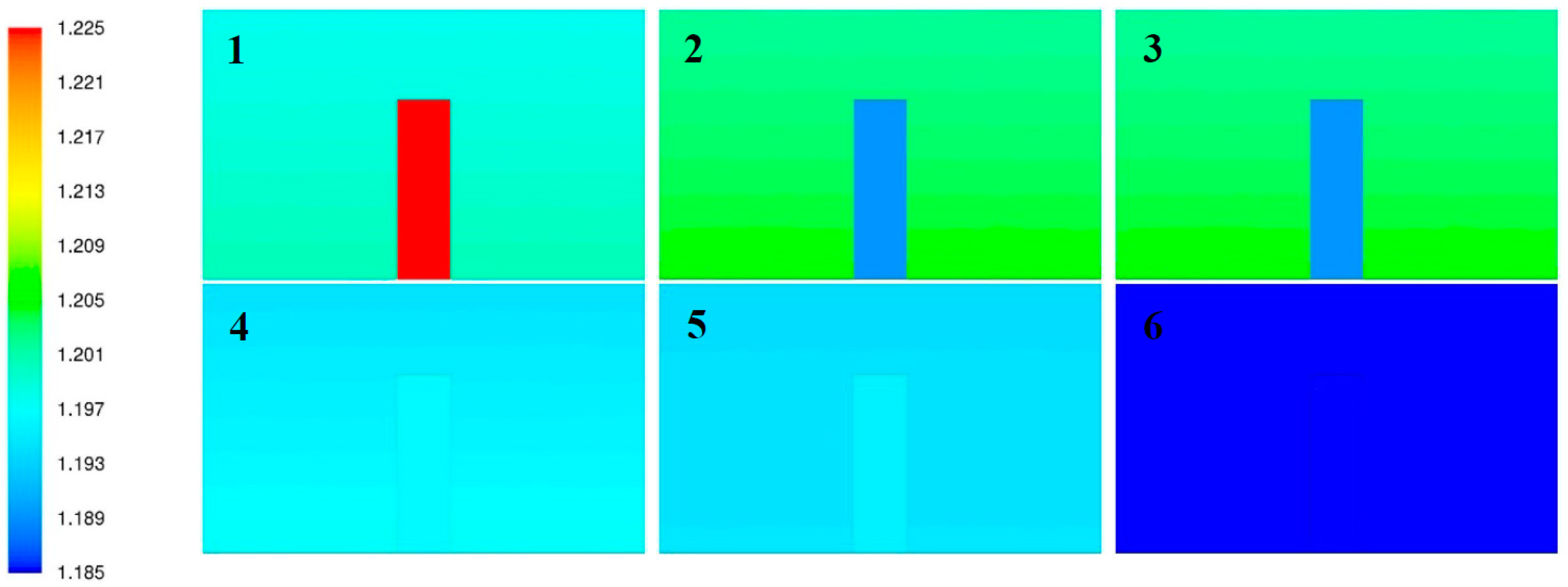
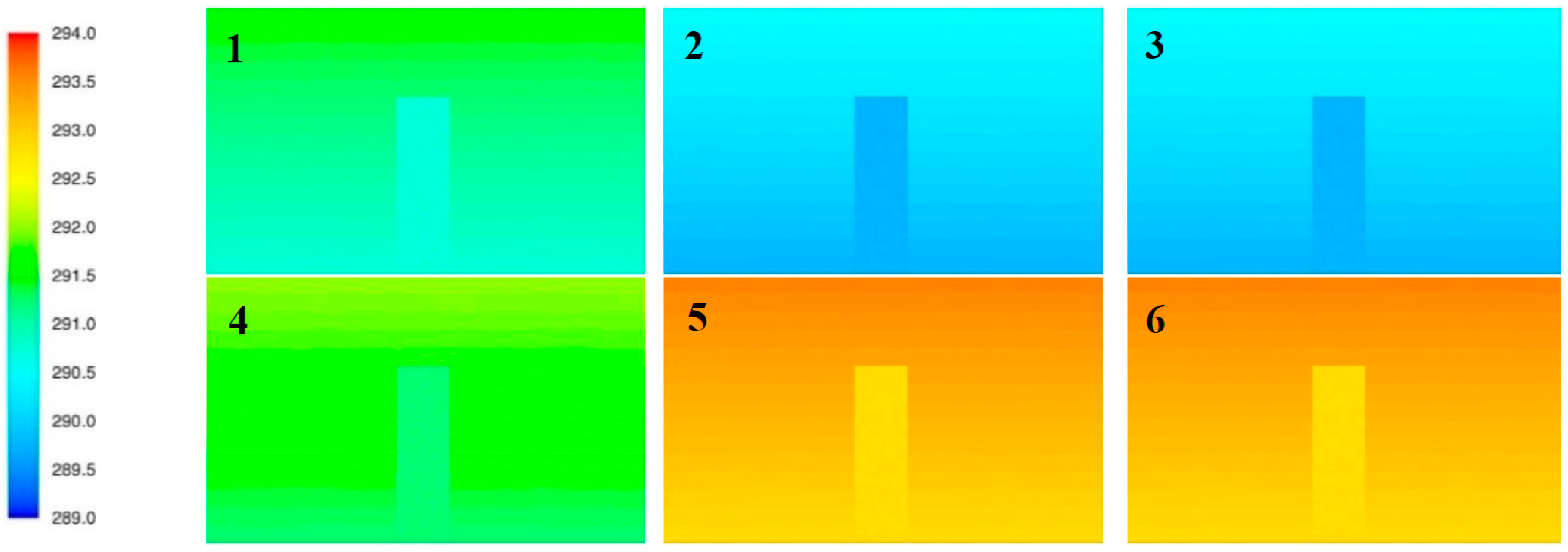
3.1. Overview of the Results of Numerical Modelling

CFD simulations were performed for standard fire-extinguishing gases composed of Ar = 50% v/v and N₂ = 50% v/v (type IG 55), and Ar = 0% v/v and N₂ = 100% v/v (type IG 100), and for four other fire-extinguishing mixtures with densities similar to the density of air. The additional mixtures were based on the work presented in [11], and normalised to the retention concentration of the gas of 13% in volume. The Oxygen concentration was measured at five points, as shown on Figure 2.

The retention time values identified numerically based on the obtained changes in the distribution of the fire-extinguishing gas concentration ranged from 50 to 869 s (

Table 2. Retention times of fire-extinguishing gases.

No.	Ar [%v/v]	N2 [%v/v]	Δρ = dm − d0 [kg/m3]	Retention Time (Experiment) TR [s]	Retention Time (Stand. Model) tRn [s]	Retention Time—CFD [s]	Relative Errors in Relation to the Experiment [11]
							Standard Model	CFD
1	50	50	(+) 0.192	57	60.8	50	−6.67	12.28
2	0	100	(−) 0.039	119	136.7	135	−14.87	−13.45
3	10	90	(+) 0.007	768	272	338	64.58	55.99
4	6.9	93.1	(−) 0.007	186	325.1	654	−74.78	−251.61
5	7.8	92.2	(−) 0.003	255	1563	396	−512.94	−55.29
6	7.5	92.5	(−) 0.004	210	640.6	869	−205.05	−313.8

(+)—fire-extinguishing gas heavier than air, (−)—fire-extinguishing gas lighter than air.

). In order to compare the accuracy of the models, a relative error at the retention time identification for each kind of fire-extinguishing gas respectively was calculated.

The retention time is not a physical value that would characterize the fire safety of a premise, but purely a measurement of the time that passes from the release and the achievement of extinguishing concentration of the gas within the compartment, to the moment when the oxygen concentration (v/v) does exceed a 13% value in one of the measurement points. This means that this value of time is not explicitly calculated by the CFD, but can be estimated based on the local concentration of extinguishing gas or oxygen. The differences in the assessed retention time for gasses with a small value of Δρ (difference of density between the extinguishing gas and the ambient air) are large. However, the CFD model presents values closer to the experiment than the standard model, Figure 9. Moreover, as can be noticed in the presented further time-plots of the oxygen concentration, this is not only a difference in the estimation of the time, but a significant difference in the estimation of the concentration or flow within the room. As shown in Figure 10, even though the retention time criterion is passed before the 1200th second in all of the simulations, for scenarios 2–6, a significant part of the premise is still protected with an effective concentration of extinguishing gas. The differences between different gasses may be a result of different flow rate through leakages, due to the differences in hydrostatic pressure. Figure 11 presents the maximum flow velocity measured at the leakages for different values of Δρ. It can be noted that for large Δρ = 0.192 kg/m³, the velocity is close to 0.8 m/s, while for the gasses with density very close to the density of air this velocity is below 0.1 m/s. With such low air flow velocity, a small change in the velocity may cause significant change in the retention time—which may be an explanation to the discrepancies found between CFD and experiment for gasses with small value of Δρ. The user should be aware that in this scenario, the CFD model is very sensitive to the initial conditions.

The Oxygen concentration was measured in all of the measurement points (the example is shown on Figure 12), however the measurements on the points far from the interface between layers show small change in concentration in time. Thus, for practical reasons in the following text, all considerations will relate to the measurement point, on which the concentration of Oxygen first reached 13% v/v.

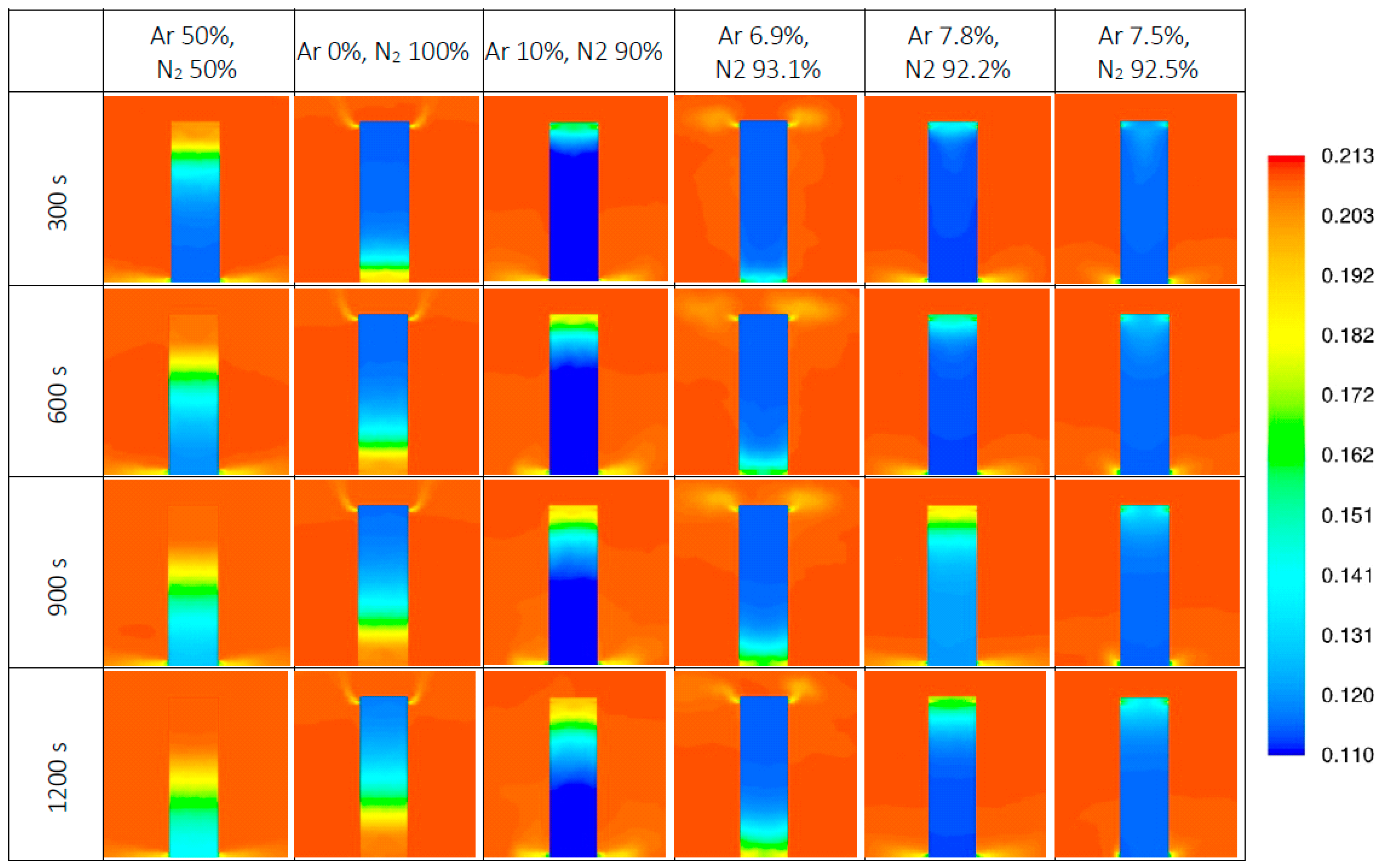
3.2. The results for Standard Mixtures

The results of flow modelling standard mixtures—IG 55 and IG 100—as presented in Figure 13 and Figure 14. These mixtures have a large value of Δρ, which means they are much heavier or lighter than the surrounding air. For these mixtures, the flow modelled by CFD method is well represented in the early stage of the—up to an O₂ concentration of approx. 14%. In both cases, the O₂ concentration in the CFD simulation is within 10% of the value measured in the experiment. In the following part of the experiment, higher discrepancies in this measurement are observed. However, the difference between experiment and CFD does not exceed 15%. In the case of Ar 0% v/v and N₂ 100% v/v mixture, the change of O₂ concentration in experiment seems to be parabolic, while in the late stage of CFD, this change is linear. We interpret this discrepancy as a difference in the physical representation of the interface layer between layers (gas and clean air). In numerical simulations, the change of density in height of the boundary layer was linear, while in experiments this could be exponential. Due to limited amount of measurement points in the experimental study [11], it is difficult to further investigate this, however this may be an interesting subject for future work. It must be also noted that related to the treatment of the boundary layer, there are differences between standard models—some describe it as sharp interface, while other models use wide interface layer. This problem was discussed in depth in [11].

For the flow of gasses with a large value of Δρ, the numerical model shown “wide division line” between air and extinguishing gas, while for the low values of Δρ the boundary between layers was narrow.

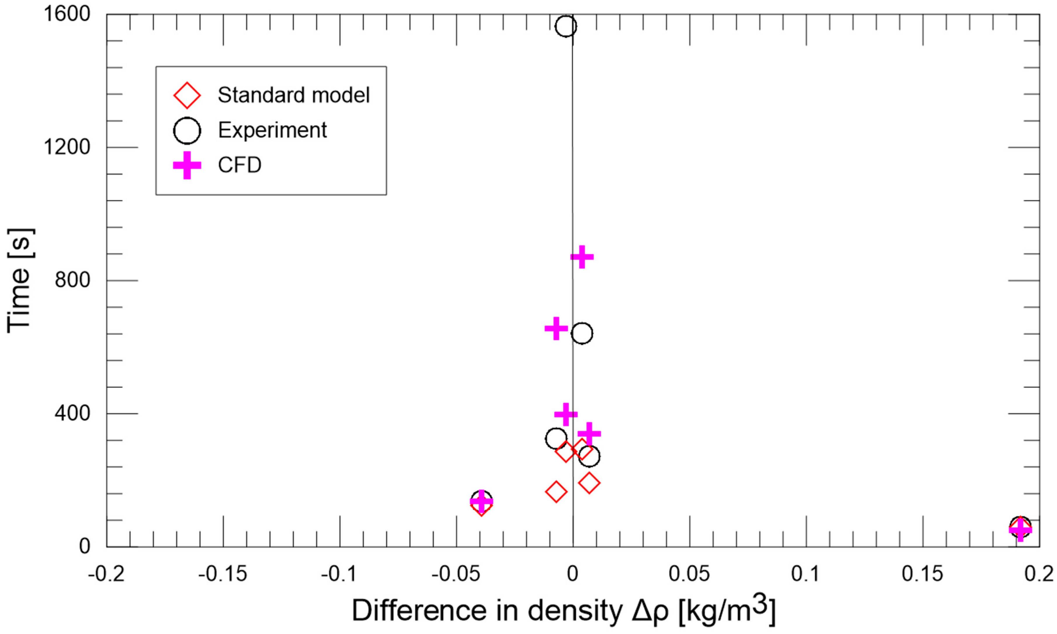
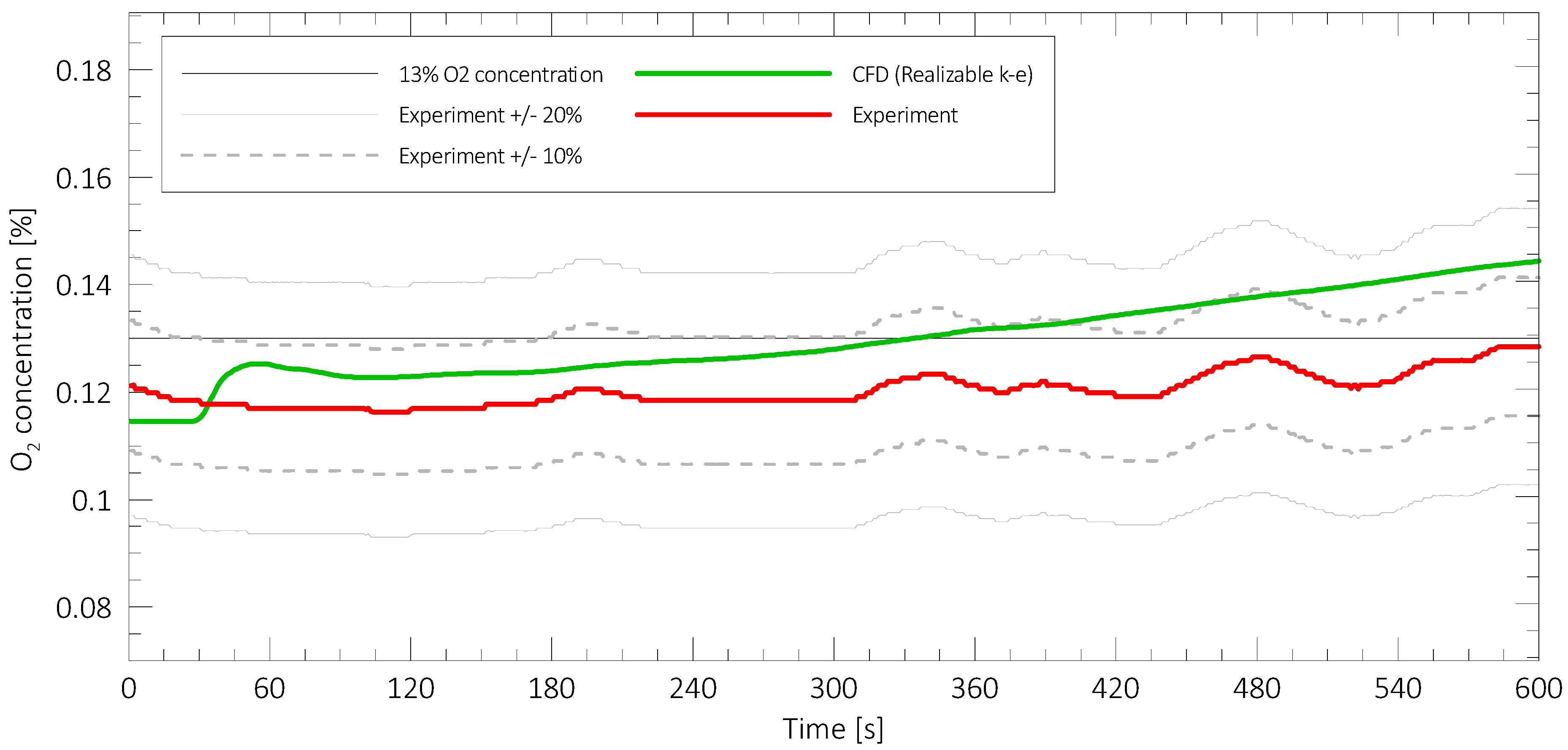
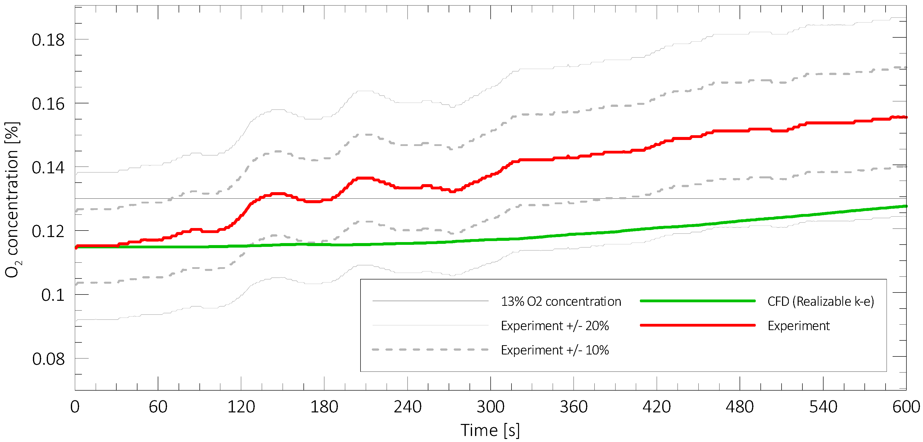
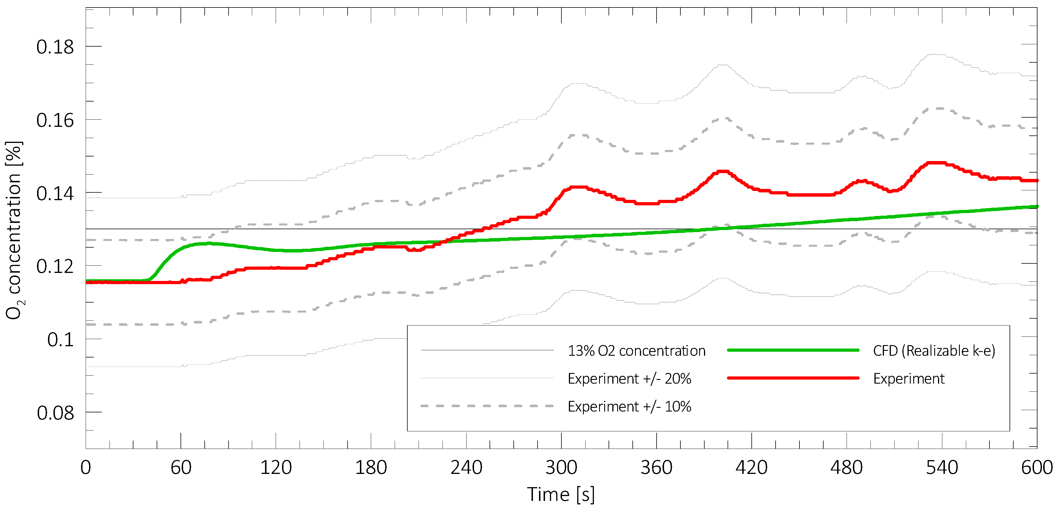
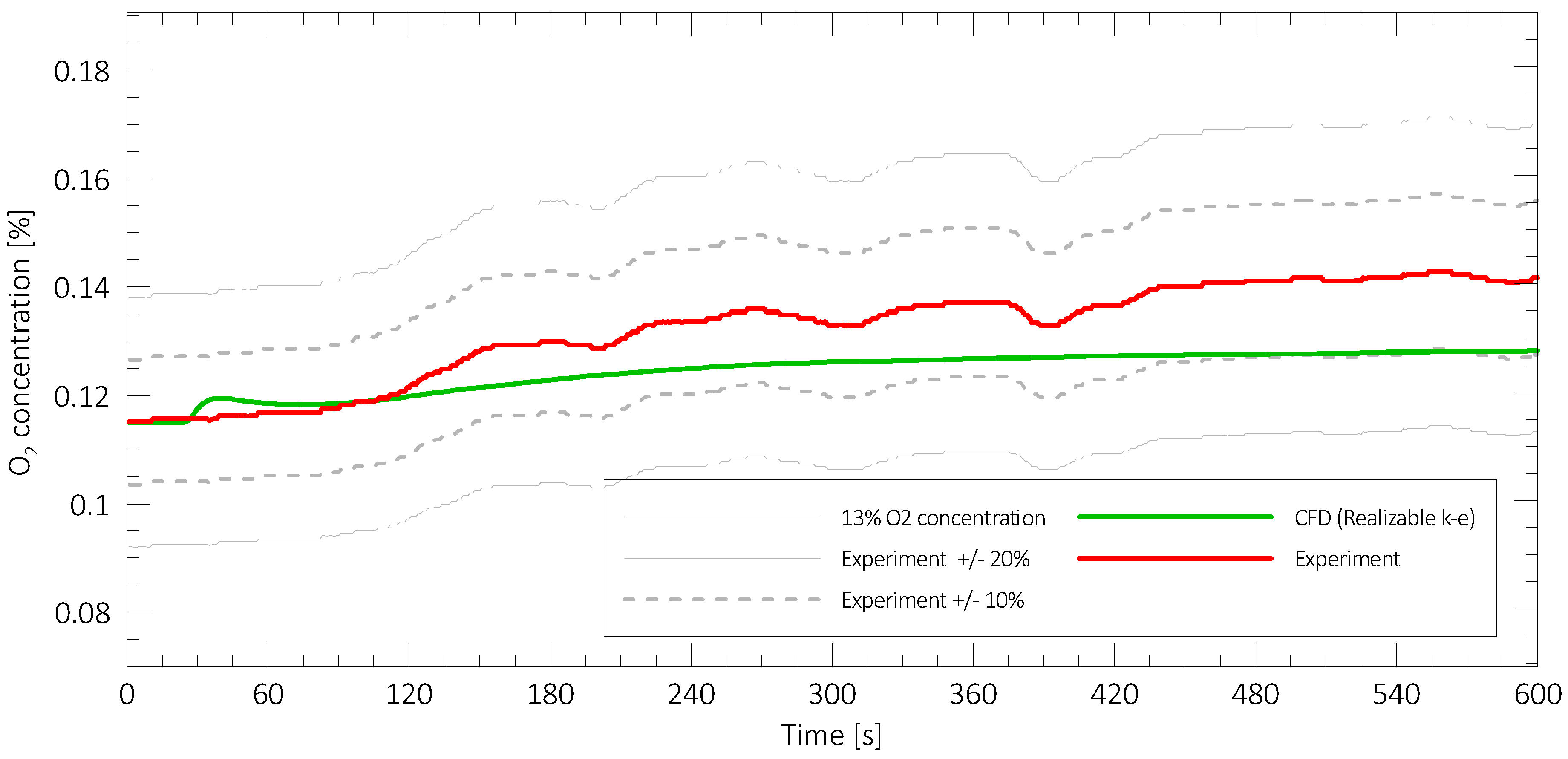
3.3. The results for Mixtures with a Small Value of Δρ

For mixtures with a small value of Δρ, Figure 15, Figure 16, Figure 17 and Figure 18, it can be noted that prediction of the change in O₂ concentration is difficult for the CFD model, which is also a well-known problem for standardised models. However, in 3 out of 4 tested mixtures, the errors are smaller than 10% of the value measured in the experiment. In the case of Ar 6.9% v/v and N₂ 93.1% v/v mixture, the error is close to 20%, but the CFD well represents the trend and the rate of mixing. This may indicate that in this particular case the initialisation method had a significant influence over the results. It must be noted that in the CFD analysis the calculations were initialised with uniform gas and O₂ concentration within the whole compartment, while in the experiment this was the outcome of the discharge.

The analysed numerical models described the processes of the fire-extinguishing gas flow through a room in a way similar to the actual phenomenon observed during the experiment. The direction of the flow (upward or downward) was well represented. For the mixtures Ar 7.8% v/v and N₂ 92.2% v/v and Ar 7.5% v/v and N₂ 92.5% v/v, the difference of Δρ at the top and the bottom of the compartment was significant, and that caused a downwards flow, despite the fact that average Δρ was negative. In some of the experiments with values of Δρ close to 0, in the late stage of the experiment it was observed that the mixing of air and extinguishing gas occurred at both top and the bottom of the compartment. This behaviour was not observed in the CFD simulations.

Despite the good representation of the O₂ concentration (v/v) in the protected compartment, it is difficult to point out the moment at which the retention time ends. The O₂ concentration (v/v) is close to the value of 13% for a long period, and the sole moment when this value is obtained says little about the conditions in the compartment. This poses a problem only when the results of CFD are directly compared to the results of standard calculation methods. For practical use of the CFD method in the design of the gaseous extinguishing system, the O₂ concentration (v/v) in the compartment is represented with sufficient accuracy. As there are no guidelines for this particular use of numerical modelling, we recommend following the recommendations of OECD [26]. Some useful considerations on CFD modelling in fire safety engineering may be also found in [47].

4. Discussion

Despite the applied simplifications in the numerical analysis and the lack of discharge modelling, the gas flow image preserved the features characteristic of the post-discharge fire-extinguishing gas movement in protected rooms. The modelled changes in the gas concentration in time do not deviate from the actual values by more than 20% (and in most cases not more than 10%), which can be considered a satisfactory value. Moreover, in specific cases, the numerical models rendered results closer to the experimental values than the retention time values identified with the standard model. Despite the discrepancies in the identified retention time values, the results of numerical calculations generally indicate that the model was close to the experiment, which can be interpreted as confiscation of the proper resolution of the phenomena that occur during the fire-extinguishing gas flow through the room. Based on these results, it may be considered reasonable to omit the discharge modelling in practical cases, as a method for optimising computational resources. However, one should be aware of the limitations of such an approach—uniform gas concentration within the domain is assumed, and not estimated as a result of the discharge simulation. If there is a risk of non-uniform gas distribution (e.g., non-uniform placement of nozzles, complex geometries), it may be necessary to resolve the discharge.

The numerical model used herein could be further improved to reduce the error in the identified retention time value, however since the retention time is not the perfect measure of the real performance of the low Δρ gas mixtures, these efforts seem futile. For mixtures with a large value of Δρ, both the retention time and the O₂ concentration were predicted with very good accuracy.

This study shows a large potential in CFD modelling for assessment of the real fire-safety level in the protected space, not based on a time index, but rather on a realistic image of gas-mixing and resulting gas concentrations within the space. Use of the CFD method in place of standardised calculation methods gives a better overview of the fire safety of protected compartment, through a better presentation of the retention process instead of an arbitrary time value given by standardised methods. The retention time value does not give any information on what are the conditions within the compartment after this time passes. The universal application, regardless of the studied compartment, would be an important advantage of CFD models over standard models. Correct validation of the CFD model can help to obtain a model relevant for almost any scope of application.

5. Conclusions

The prolonged suppression effect of gaseous extinguishing systems, achieved by maintaining a high concentration of the extinguishing gas in the post-discharge phase, is critical for the safety of protected premises. High gas concentration prevents fire recurrence and spreading and allows longer rescue operation time. In order to design a gaseous extinguishing system that can maximise this retention time, a simplified CFD approach was proposed. The simplifications were in the omission of the complicated discharge phase, based on the assumption that after discharge, the flow field within the protected domain is stable and the gas mixing is driven mainly by turbulent flow near leakages, hydrostatic pressure and buoyant forces in the layer and gas dispersion.

To verify this concept, we performed CFD calculations of extinguishing gases retention processes, referring to a previous experimental study [11]. Both physical and numerical experiments were performed in an idealised test array, that represented a difficult case of protected casing: high (slender), narrow and with a large leakage to volume ratio. The experiments can be considered representative for industrial casings of servers, 3D printers and other small-sized equipment. The test compartment can also be partially representative of larger compartments, because of the large leakage to volume, and leakage to floor area ratios. In typical compartments, the leakage-volume ratios are lower, and the distribution of the leakage in the height of the room is uneven. For more generalised conclusions, tests on a larger scale must be performed. This study did not include any heat or airflow sources (fans, radiators, power supply units, etc.) that can be sources of flow disturbances inside the rig. However, contrary to existing analytical models, it can be expected that the CFD solver should be able to model the thermal plumes and forced ventilation along the retention of the extinguishing gas.

The verification of initial conditions on the results of numerical modelling was performed based on a comparative analysis of (1) the values of gas concentration distribution obtained by computer simulations with the results of physical experiments and (2) the value of retention time based on the oxygen concentration on the most onerous sensor. The completed tests helped to identify the validity of the CFD methods, simplified about the gaseous discharge, to describe the fire-extinguishing gas outflow from the protected compartment. Application of the CFD methods does not mean the elimination of the theoretical and experimental approaches, but can be used complementary to them.

For high Δρ gas mixtures, the retention time estimated through CFD was close to the measured in the experiment or estimated with standardised methods. For low Δρ gas mixtures, high discrepancies were observed, due to the difficulties in predicting the moment of time in which the value of 13% oxygen concentration in volume was exceeded (the measured value was close to 13% for a long period). The inability to precisely estimate the retention time value for low Δρ gas mixtures does not pose a problem in the practical use of CFD for the design of gaseous systems.

In this series, the turbulent model did not influence the results in a significant way—all of the tested closure approaches gave similar results, regarding the retention time and oxygen concentrations. This could mean that simplified models (standard and Realizable k-ε) are viable and recommended from the cost-efficiency point of view. However, a significant effect of the coarse mesh resolution was observed. Thus, the numerical mesh for the retention modelling should be chosen after a mesh sensitivity study, which proves that further mesh adjustment does not change the quantitative results in a significant way.

In future, the use of computational fluid dynamics (CFD) can become a new important engineering tool in studies covering the protection of premises with fire-fighting gases. The possibility of selecting the right mixture of fire-fighting gases can help improve fire safety at reduced costs.

References

1. Milke, J. Fire protection as the underpinning of good process safety programs. J. Loss Prev. Process Ind. 2016, 40, 329–333. [Google Scholar] [CrossRef]
2. Węgrzyński, W.; Sulik, P. The philosophy of fire safety engineering in the shaping of civil engineering development. Bull. Pol. Acad. Sci. Tech. Sci. 2016, 64, 719–730. [Google Scholar] [CrossRef] [Green Version]
3. Wang, B.; Rao, Z.; Xie, Q.; Wola, P. Brief review on passive and active methods for explosion and detonation suppression in tubes and galleries. J. Loss Prev. Process Ind. 2017, 49, 280–290. [Google Scholar] [CrossRef]
4. Wang, Z.; Wang, W.; Wang, Q. Optimization of water mist droplet size by using CFD modeling for fire suppressions. J. Loss Prev. Process Ind. 2016, 44, 626–632. [Google Scholar] [CrossRef]
5. Jenft, A.; Collin, A.; Boulet, P.; Pianet, G.; Breton, A.; Muller, A. Experimental and numerical study of pool fire suppression using water mist. Fire Saf. J. 2014, 67, 1–12. [Google Scholar] [CrossRef]
6. Rie, D.-H.; Lee, J.-W.; Kim, S. Class B Fire-Extinguishing Performance Evaluation of a Compressed Air Foam System at Different Air-to-Aqueous Foam Solution Mixing Ratios. Appl. Sci. 2016, 6, 191. [Google Scholar] [CrossRef]
7. Buchlin, J. Mitigation of industrial hazards by water spray curtains. J. Loss Prev. Process Ind. 2017, 50, 91–100. [Google Scholar] [CrossRef]
8. Węsierski, T.; Majder-Łopatka, M. Comparison of Water Curtain Effectiveness in the Elimination of Airborne Vapours of Ammonia, Acetone, and Low-Molecular Aliphatic Alcohols. Appl. Sci. 2018, 8, 1971. [Google Scholar] [CrossRef]
9. Abramowicz, M.; Kowalski, R. The influence of short time water cooling on the mechanical properties of concrete heated up to high temperature. J. Civ. Eng. Manag. 2005, 11, 85–90. [Google Scholar] [CrossRef]
10. Węgrzyński, W.; Vigne, G. Experimental and numerical evaluation of the influence of the soot yield on the visibility in smoke in CFD analysis. Fire Saf. J. 2017, 91, 389–398. [Google Scholar] [CrossRef]
11. Kubica, P.; Czarnecki, L.; Boroń, S.; Węgrzyński, W. Maximizing the retention time of inert gases used in fixed gaseous extinguishing systems. Fire Saf. J. 2016, 80, 1–8. [Google Scholar] [CrossRef]
12. Du, D.; Shen, X.; Feng, L.; Hua, M.; Pan, X. Efficiency characterization of fire extinguishing compound superfine powder containing Mg(OH)2. J. Loss Prev. Process Ind. 2019, 57, 73–80. [Google Scholar] [CrossRef]
13. Shebeko, A.Y.; Shebeko, Y.N.; Zuban, A.V.; Navzenya, V.Y. An experimental investigation of an inertization effectiveness of fluorinated hydrocarbons in relation to premixed H2-N2O and CH4-N2O flames. J. Loss Prev. Process Ind. 2013, 26, 1639–1645. [Google Scholar] [CrossRef]
14. Chaudhari, P.; Mashuga, C.V. Partial inerting of dust clouds using a modified standard minimum ignition energy device. J. Loss Prev. Process Ind. 2017, 48, 145–150. [Google Scholar] [CrossRef]
15. Ouyang, D.; Liu, J.; Chen, M.; Wang, J. Investigation into the Fire Hazards of Lithium-Ion Batteries under Overcharging. Appl. Sci. 2017, 7, 1314. [Google Scholar] [CrossRef]
16. Ouyang, D.; Liu, J.; Chen, M.; Weng, J.; Wang, J. An Experimental Study on the Thermal Failure Propagation in Lithium-Ion Battery Pack. J. Electrochem. Soc. 2018, 165, A2184–A2193. [Google Scholar] [CrossRef]
17. Chen, M.; Liu, J.; Dongxu, O.; Cao, S.; Wang, Z.; Wang, J. A Simplified Analysis to Predict the Fire Hazard of Primary Lithium Battery. Appl. Sci. 2018, 8, 2329. [Google Scholar] [CrossRef]
18. ANSYS. ANSYS Fluent 14.5.0—Technical Documentation; ANSYS: Canonsburg, PA, USA, 2014. [Google Scholar]
19. Boroń, S.; Kubica, P. Application of Computational Fluid Dynamics CFD for Modeling of Protection of Premises by Fixed Gaseous Extinguishing System (in Polish). Bezpieczeństwo Tech. Pożarnicza 2016, 42, 151–157. [Google Scholar]
20. Wnęk, W.; Kubica, P. Analysis of distribution of oxygen concentrations during fire extinction in the enclosure by nitrogen with forced air condition. Bezpieczeństwo Tech. Pożarnicza 2011, 24, 65–79. (In Polish) [Google Scholar]
21. Kubica, P. Retention Time of Gaseous Extinguishing Systems in the Fire Safety of Compartments; Instytut Techniki Budowlanej: Warsaw, Poland, 2014. (In Polish) [Google Scholar]
22. NFPA 2001 Standard on Clean Agent Fire Extinguishing Systems; NFPA: Quincy, MA, USA, 2012.
23. ISO 14520-1 Gaseous Fire-Extinguishing Systems—Physical Properties and System Design—Part 1: General Requirements; ISO: Geneva, Switzerland, 2015.
24. BS EN 15004-1:2008 Fixed Firefighting Systems—Gas Extinguishing Systems. Design, Installation and Maintenance; BSI: London, UK, 2008.
25. Genge, C. Clean agent enclosurer desgin optimization for peak pressures and agent retention. In Proceedings of the SFPE Engineering Technology Conference, Portland, OR, USA, 24–25 October 2011. [Google Scholar]
26. OECD. NEA Best Practice Guidelines for the Use of CFD in Nuclear Reactor Safety Application—Revision. In NEA/CSNI/R(2014)11; OECD: Paris, France, 2015. [Google Scholar]
27. McGrattan, K.; Miles, S. Modeling Fires Using Computational Fluid Dynamics (CFD). In SFPE Handbook of Fire Protection Engineering; Springer: New York, NY, USA, 2016; pp. 1034–1065. [Google Scholar]
28. Merci, B.; Beji, T. Fluid Mechanics Aspects of Fire and Smoke Dynamics in Enclosures; CRC Press: Boca Raton, FL, USA, 2016. [Google Scholar]
29. Chung, T.J. Computational Fluid Dynamics; Cambridge University Press: Cambridge, UK, 2002. [Google Scholar]
30. Ferziger, J.H.; Peric, M. Computational Methods for Fluid Dynamics; Springer: New York, NY, USA, 2002. [Google Scholar]
31. McGrattan, K.; McDermott, R.; Floyd, J.; Hostikka, S.; Forney, G.; Baum, H. Computational fluid dynamics modelling of fire. Int. J. Comput. Fluid Dyn. 2012, 26, 349–361. [Google Scholar] [CrossRef]
32. Wahlqvist, J.; van Hees, P. Implementation and validation of an environmental feedback pool fire model based on oxygen depletion and radiative feedback in FDS. Fire Saf. J. 2016, 85, 35–49. [Google Scholar] [CrossRef]
33. Król, M.; Król, A. Multi-criteria numerical analysis of factors influencing the efficiency of natural smoke venting of atria. J. Wind Eng. Ind. Aerodyn. 2017, 170, 149–161. [Google Scholar] [CrossRef]
34. Król, A.; Król, M. Study on Hot Gases Flow in Case of Fire in a Road Tunnel. Energies 2018, 11, 590. [Google Scholar] [CrossRef]
35. Tauseef, S.M.; Rashtchian, D.; Abbasi, S.A. CFD-based simulation of dense gas dispersion in presence of obstacles. J. Loss Prev. Process Ind. 2011, 24, 371–376. [Google Scholar] [CrossRef]
36. Dong, L.; Zuo, H.; Hu, L.; Yang, B.; Li, L.; Wu, L. Simulation of heavy gas dispersion in a large indoor space using CFD model. J. Loss Prev. Process Ind. 2017, 46, 1–12. [Google Scholar] [CrossRef]
37. Yang, S.; Jeon, K.; Kang, D.; Han, C. Accident analysis of the Gumi hydrogen fluoride gas leak using CFD and comparison with post-accidental environmental impacts. J. Loss Prev. Process Ind. 2017, 48, 207–215. [Google Scholar] [CrossRef]
38. Luo, T.; Yu, C.; Liu, R.; Li, M.; Zhang, J.; Qu, S. Numerical simulation of LNG release and dispersion using a multiphase CFD model. J. Loss Prev. Process Ind. 2018, 56, 316–327. [Google Scholar] [CrossRef]
39. Middha, P.; Hansen, O.R.; Storvik, I.E. Validation of CFD-model for hydrogen dispersion. J. Loss Prev. Process Ind. 2009, 22, 1034–1038. [Google Scholar] [CrossRef]
40. Mcnay, J.; Hilditch, R. Evaluation of computational fluid dynamics (CFD) vs. target gas cloud for indoor gas detection design. J. Loss Prev. Process Ind. 2017, 50, 75–79. [Google Scholar] [CrossRef]
41. Blocken, B. LES over RANS in building simulation for outdoor and indoor applications: A foregone conclusion? Build. Simul. 2018, 11, 821–870. [Google Scholar] [CrossRef]
42. Gibson, M.M.M.; Launder, B.E.E. Ground effects on pressure fluctuations in the atmospheric boundary layer. J. Fluid Mech. 1978, 86, 491–511. [Google Scholar] [CrossRef]
43. Launder, B.E. Second-moment closure: Present… and future? Int. J. Heat Fluid Flow 1989, 10, 282–300. [Google Scholar] [CrossRef]
44. Pope, S.B. Ten questions concerning the large-eddy simulation of turbulent flows. New J. Phys. 2004, 6, 35. [Google Scholar] [CrossRef]
45. Wilcox, D.C. Turbulence Modeling for CFD, 3rd ed.; DCW Industries Inc.: La Cañada, CA, USA, 2006. [Google Scholar]
46. Peacock, R.D.; Reneke, P.A.; Davis, W.D.; Jones, W.W. Quantifying fire model evaluation using functional analysis. Fire Saf. J. 1999, 33, 167–184. [Google Scholar] [CrossRef]
47. Węgrzyński, W.; Lipecki, T.; Krajewski, G. Wind and Fire Coupled Modelling—Part II: Good Practice Guidelines. Fire Technol. 2018, 54, 1443–1485. [Google Scholar] [CrossRef]
Figure 1. Three stages of the release of extinguishing gas into the compartment. (A) Flow field in the compartment dominated by fire growth and smoke buoyancy, prior to release, (B) release of the fire extinguishing gas, (C) stabilized flow field in the compartment filled with extinguishing gas after the discharge. Stage (C) is modelled in this study.
Applsci 09 00663 g001
Figure 2. Diagram of the test rig used as the reference for the numerical experiments [11,21].
Applsci 09 00663 g002
Figure 3. Initial conditions for numerical calculations—comparison of the density (1.185–1.225 g/m3) of air outside the chamber with the density of fire-extinguishing gas and air mixture inside the chamber; the scenario numbers refer to Table 1.
Applsci 09 00663 g003
Figure 4. Initial conditions for numerical calculations—comparison of the air temperature (289–294 K) outside the chamber with the temperature of the mixture of fire-extinguishing gas and air inside the chamber; the scenario numbers refer to Table 1.
Applsci 09 00663 g004
Figure 5. Changes in oxygen concentration (v/v) on the probe No. 1, indicating the end of the retention time during experimental tests and computational fluid dynamics (CFD) simulations, fire-extinguishing gas Ar 50% v/v and N2 50% v/v.
Applsci 09 00663 g005
Figure 6. Changes in oxygen concentration (v/v) on the probe No. 5, indicating the end of the retention time during experimental tests and CFD simulations, fire-extinguishing gas Ar 0% v/v and N2 100% v/v.
Applsci 09 00663 g006
Figure 7. Results of mesh sensitivity study for Reynolds-Averaged Navier–Stokes (RANS) k-ε (Realizable) turbulence model and IG 55 mixture (50% Ar, 50% N2)—oxygen concentration (v/v) at lowest measuring element in the experiment and numerical study.
Applsci 09 00663 g007
Figure 8. A general overview of the mesh used in the numerical experiment.
Applsci 09 00663 g008
Figure 9. Comparison of the retention time estimate in experiment [11], standard model calculations and CFD analysis for different values of Δρ.
Applsci 09 00663 g009
Figure 10. Oxygen concentration distribution in the test chamber in chosen time points for all evaluated scenarios (Table 1). In cases 2 and 4 the gas escapes the protected chamber through top leakage. Prolonged protective effect of gas mixtures 3–6 may be noted.
Applsci 09 00663 g010
Figure 11. Comparison of the maximum flow velocity measured at leakages in CFD analysis for different values of Δρ.
Applsci 09 00663 g011
Figure 12. Changes in oxygen concentration (v/v) on all of the measurement points for fire-extinguishing gas Ar 0% v/v and N2 100% v/v.
Applsci 09 00663 g012
Figure 13. Changes in oxygen concentration (v/v) on the probe No. 1, indicating the end of the retention time during experimental tests and CFD simulations, fire-extinguishing gas Ar 50% v/v and N2 50% v/v.
Applsci 09 00663 g013
Figure 14. Changes in oxygen concentration (v/v) on the probe No. 5, indicating the end of the retention time during experimental tests and CFD simulations, fire-extinguishing gas Ar 0% v/v and N2 100% v/v.
Applsci 09 00663 g014
Figure 15. Changes in oxygen concentration (v/v) on the probe No. 1, indicating the end of the retention time during experimental tests and CFD simulations, fire-extinguishing gas Ar 10% v/v and N2 90% v/v.
Applsci 09 00663 g015
Figure 16. Changes in oxygen concentration (v/v) on the probe No. 5, indicating the end of the retention time during experimental tests and CFD simulations, fire-extinguishing gas Ar 6.9% v/v and N2 93.1% v/v.
Applsci 09 00663 g016
Figure 17. Changes in oxygen concentration (v/v) on the probe No. 1, indicating the end of the retention time during experimental tests and CFD simulations, fire-extinguishing gas Ar 7.8% v/v and N2 92.2% v/v.
Applsci 09 00663 g017
Figure 18. Changes in oxygen concentration (v/v) on the probe No. 1, indicating the end of the retention time during experimental tests and CFD simulations, fire-extinguishing gas Ar 7.5% v/v and N2 92.5% v/v.
Applsci 09 00663 g018