Optimal Scheduling of Hydro–PV–Wind Hybrid System Considering CHP and BESS Coordination

Abstract

Coordination of a hydropower, combined heat and power (CHP), and battery energy storage system (BESS) with multiple renewable energy sources (RES) can effectively reduce the adverse effects of large-scale renewable energy integration in power systems. This paper proposes a concept of a renewable-based hybrid energy system and puts forward an optimal scheduling model of this system, taking into account the cost of operation and risk. An optimization method is proposed based on Latin hypercube sampling, scene reduction, and piecewise linearization. Firstly, a large number of samples were generated with the Latin hypercube sampling method according to the uncertainties, including the renewable resources availability, the load demand, and the risk aversion coefficients, and the generated samples were reduced with a scene reduction method. Secondly, the piecewise linearization method was applied to convert nonlinear constraints into linear to obtain the best results of each scene. Finally, the performance of the proposed model and method was evaluated based on case studies with real-life data. Results showed that the renewable-based hybrid system can not only reduce the intermittent and volatility of renewable resources but also ensure the smooth of tie-line power as much as possible. The proposed model and method are universal, feasible, and effective.

1. Introduction

In recent years, with the increasing attention on global climate change and sustainable development, the penetration of renewable energy resources (RES) has steadily grown in the global electricity market. As renewable energy sources are starting to play a prominent role in revolutionizing modern power systems, the impact on their operation and reliability no longer goes unnoticed and neglected. However, because of their variability and difficult-to-predict nature, renewable resources are always considered an unreliable resource, and their scheduled generation cannot be ensured [1,2]. Therefore, it seems that after overcoming the impediments related to the cost, the next problem which should be solved is the reliable and economically justifiable integration of RES into the power system. This is especially important in the case of RES such as wind and solar, which tend to exhibit a significant temporal and spatial variability [3]. The problems of RES integration into the power system have been studied in several studies [4,5,6].

In order to provide stable generation, coordination of several kinds of energy sources may be an effective way to overcome these disadvantages above. Because of the large scale and good regulation performance, hydroelectric power can effectively restrain the fluctuations in wind and photovoltaic generation to improve their stabilities. Based on integrated technology, establishing a hydro–photovoltaic–wind hybrid system is seen as a promising method to realize the conception [7,8]. Malakar et al. [9] performed the coordinating strategy of a wind–hydro hybrid system connected grid under frequency-based pricing. Reference [10] studied the portfolios of multiple energy sources considering the complementarity between wind power and photovoltaics. The portfolios may play an important role in reducing the fluctuations and intermittency to improve the reliability of individual generation [11]. A method to solve the optimal power flow problem with different probability density functions for wind and solar power was suggested by Reddy [12]. A stochastic day-ahead optimal strategy for a wind–hydro system was presented by Biswas [13] considering the risk of the system. References [14,15,16,17] studied the models of the wind–hydro hybrid system to reduce the cost of imbalances. Compared with renewable resources, combined heat and power (CHP) systems are highly controllable and have quite quick rates. Therefore, these systems with CHP are flexible and can be used to ensure balance and improve the stability of RES integration into the power system [15]. The models for determining the strategy for optimal operation and trading of CHP systems have many relevant studies. CHP systems can be optimized based on different optimization criteria, such as energy savings, cost reduction, minimum environmental impact, or a combination of all of these [16]. Several methods and criteria have been proposed in the literature for optimization of the size and operation of CHP systems [17,18,19,20,21]. References [22,23] proposed deterministic optimization models, while References [24,25,26,27] presented stochastic programming models of CHP systems due to their ability to approach various uncertainties in CHP system operation. References [28,29] proposed an economic dispatch model that included CHP units, with a comprehensive survey reported [30,31,32]. Lai [33] designed a CHP system by integrating the thermal storage techniques considering the uncertainty of demand. Taking the variation of demands and prices into account, Carpaneto et al. [34] solved the best CHP plan based on the decision theory concepts. Zapata et al. [35] promoted an aggregation model of a CHP–photovoltaic (PV) hybrid system under uncertainty in the Belgian market. In addition, due to the ability of energy storage, the battery energy storage system (BESS) is generally regarded as an effective tool to deal with the intermittent characteristics of RES. Liao [36] proposed an optimization method for sizing and scheduling BESS and the smart inverter (SI) of a photovoltaic (PV) system to ensure the PV system owner’s investment returns and to assist the distribution system operator (DSO) in adjusting the voltages. Chettibi [37] proposed an intelligent control strategy for a grid connected hybrid energy generation system consisting of photovoltaic (PV) panels, fuel cell (FC) stack, and BESS. Branco [38] put forward the integration of RES considering the installation of a battery energy storage system (BESS) into an isolated power grid to keep the costs down.

However, to our knowledge, the concept of coupling all the above energy together has not been proposed in the existing literature. In this paper, we coupled the photovoltaic modules (PV), a wind turbine (WT), battery energy storage modules (BESS), electric vehicle chargers (EV), CHP, and a hydroelectric power plant as a portfolio, in an attempt to reduce the imbalance and ultimately minimize the cost of the portfolio considering risk factor. Based on the perspective of the concept, a renewable-based hybrid energy system is proposed in the paper, and an optimal scheduling model of this system to minimize the cost of operation and risk is put forward considering multiple uncertainties, which include renewable resource volatility, the load demand, and different energy service providers’ coefficients of risk aversion. To handle this complex optimization problem, a method combining the Latin hypercube sampling, scene reduction, and piecewise linearization is proposed. A large number of samples were generated with the Latin hypercube sampling method according to the uncertainties, including the renewable resources availability, the load demand, and the risk aversion coefficients, and the generated samples were reduced with the scene reduction method. Additionally, the piecewise linearization method was applied to convert nonlinear constraints into linear to obtain the best results of each scene.

In summary, the main contributions of this paper can be listed as below:

(1)

Propose a concept of a renewable-based hybrid energy system along with a corresponding mathematical model which can be used to simulate and optimize its performance.

(2)

Introduce an optimal optimization model which focuses on minimizing the operating cost of energy service providers considering the environment as much as possible.

(3)

Investigate the distinction of uncertainty variables volatility on the energy exchange with the power grid.

(4)

Research the impact of different risk aversion coefficients on the operation of energy service providers.

The remainder of this paper is organized as follows. Section 2 formulates the mathematical model for the operation of the hybrid power system. In Section 3, the solution method is described in detail. In Section 4, numerical simulations of the proposed model are applied to a test system on real-life data, and discussions are provided accordingly. Finally, the conclusions of the paper are drawn in Section 5.

2. Coordinated Optimal Scheduling Model of Hybrid System

The proposed day-ahead optimal scheduling model of the hybrid system in this paper focuses on three issues: Firstly, a coordinated scheduling model including wind, solar, electric vehicle, battery energy storage, CHP, and pumped-storage power is proposed, considering all the operation constraints. Secondly, the different energy exchanges with the power grid due to the volatility of uncertainty variables are considered in the scheduling process. Finally, the impact of different risk aversion coefficients on the operation of the hybrid system is studied.

2.1. Description and Framework of the Hybrid Energy System

The renewable-based hybrid energy system supplied by energy service providers studied in the paper is composed of PV, WT, BESS, EV, CHP, and a hydroelectric power station. The conceptual structure of the proposed hybrid system in this paper is shown in Figure 1. The operation of multiple energy resources in the hybrid power is subjected to different constraints in the day-ahead scheduling because of their different characteristics. Due to the stochastic nature of the renewable resources, finding a way to maximize the wind and solar power at the lowest cost is the key to the optimal operation of hybrid energy system. In this situation, with the help of hydroelectric power plant, CHP and BESS, formulating an effective scheduling strategy to ensure the power balance of power system considering wind, solar, water, and other forms of energy is a major issue to be addressed.

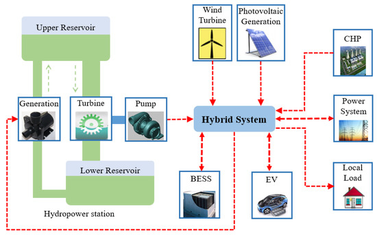
Figure 1. The conceptual structure of the considered hybrid system with energy flow.

2.2. Objective of Optimal Scheduling Model in Hybrid System

To comprehensively consider economy, environment protection, and the renewable energy consumption level, the day-ahead optimal scheduling model is constructed as follows:

$$C={\displaystyle \sum _{s=1}^{NS}{\pi }_{}^s}\left[{\displaystyle \sum _{t=1}^{NT}\left({\displaystyle \sum _{g=1}^{NG}{C}_{CHP}^{g,t,s}+C_{BESS}^{t,s}+C_{grid}^{t,s}}\right)}\right]+\beta \times CVaR$$

(1)

The above objective is to minimize the operation cost consisting of four distinct terms, including the generation cost of all CHPs, the cost of BESS, the cost of power exchange with the utility grid, and the cost of risk valued by CVaR. The indices g, t, and s represent the CHPs, time periods, and the scenarios. The objective is subject to many system equality and inequality constraints, including the power balance constraint in Equation (2), utility grid power exchange limit in Equation (3), and the constraint of risk in Equation (4). Meanwhile, these costs are calculated by the following model of different energy resources, respectively:

$$P_W^{t,s}+P_{solar}^{t,s}+P_h^{t,s}+{\displaystyle \sum _{g=1}^{NG}{P}_{CHP}^{g,t,s}}+P_{disch\arg e}^{t,s}-P_{ch\arg e}^{t,s}-P_{ev}^{t,s}+P_{grid}^{t,s}=P_{load}^{t,s}$$

(2)

$$-P_{grid}^{\max }\le P_{grid}^{t,s}\le P_{grid}^{\max }$$

(3)

$${\tau }_{}^s\ge \left[{\displaystyle \sum _{t=1}^{NT}\left({\displaystyle \sum _{g=1}^{NG}{C}_{CHP}^{g,t,s}+C_{BESS}^{t,s}+C_{grid}^{t,s}}\right)}\right]-\epsilon$$

(4a)

$$CVaR=\epsilon +\frac{1}{NS(1-c)}{\displaystyle \sum _{s=1}^{NS}{\tau }_{}^s}$$

(4b)

$${\tau }_{}^s\ge 0$$

(4c)

The power balance in Equation (2) ensures that the sum of power generated by local generations and exchanged with the utility grid matches the local load. The power exchange with the utility grid is limited by the flow limits of the associated connecting line, as presented in Equation (3). Equation (4) denotes that the factor of risk with auxiliary variables of CVaR.

2.2.1. The Model of Hydro Power Station

Hydro power is a traditional renewable clean energy. In accordance with the regulation ability of water, the hydropower station can be divided into two categories, a run-off hydropower station and a pumped storage power station. The latter has a certain capacity of reservoir, which can store the appropriate capacity of water and have a certain ability to adjust and control electricity. Therefore, we assumed the hydropower station in this paper is a pumped storage power station to complement the renewable resources effectively. The output power of the hydro unit follows a function with the water flow. The relationship can be expressed as:

$$P_h^{t,s}=F(Q_{}^{t,s})$$

(5)

$$P_h^{\min }\cdot u_h^{g,t}\le P_h^{t,s}\le P_h^{\max }\cdot u_h^{g,t}$$

(6)

$$Vo{l}_{}^{t,s}=Vo{l}_{}^{t-1,s}+R_{}^{t-1}-Q_{}^{t-1,s}-S_{}^{t-1,s}$$

(7)

$$Vo{l}_{}^{\min }\le Vo{l}_{}^{t,s}\le Vo{l}_{}^{\max }$$

(8)

$$Vo{l}_{}^{NT,s}\ge Vo{l}_{}^{end}$$

(9)

$$Vo{l}_{}^{0,s}=Vo{l}_{}^{begin}$$

(10)

The relationship between output power and the water flow is shown in Equation (5), and the output power is limited by the limits of capacity in Equation (6). Equation (7) represents the reservoir volume constraint at time t and t−1, and the right and left limits of the reservoir volume in each hour are expressed in Equation (8). Meanwhile, Equation (9) fixes the hydro reserve at the end of the period to be no less than the terminal volume limit.

2.2.2. The Model of PV and WT

Different from those of a conventional thermal power unit, the operation characteristics and uncertainties of renewable energy sources make it hard to adjust their grid power.

The output power of wind turbines is mainly determined by the speed of wind and based on the nature of the turbine’s power curve. The energy output can be expressed as follows considering the character of wind turbine operation:

$$\{\begin{array}{l}{P}_W=0,v<v_{ci}\&v>v_{co}\\ P_W=P_r\frac{\left(v-v_{ci}\right)}{\left(v_r-v_{ci}\right)}=a+bv,v_{ci}<v<v_r\\ P_W=P_r,v_r<v<v_{co}\end{array}$$

(11)

As another renewable resource, the output of solar power mainly depends on factors such as temperature, light intensity, and panel area. The output of PV can be estimated as follows:

$$P_{solar}=P_{sc}{I}_T\left[1+k\left(T_c-T_r\right)\right]/I_{sc}$$

(12a)

$$T_c=T_a+30I_T/1000$$

(12b)

Equation (12b) calculates the working temperature of photovoltaic cell components in order to estimate the output power in Equation (12a).

2.2.3. The Model of CHP

In contrast to wind and solar photovoltaic, CHP units are highly controllable. In addition, ramp-up and ramp-down times of CHP units are short. Therefore, they can be used to ensure balance and stability in the electric grid because of their flexibility. The cost of CHP as a function of output power is represented as follows:

$$C_{CHP}^{g,t,s}=F_{CHP}^{g,t,s}+y_{}^{g,t}{S}_{}^g$$

(13)

$$y_{}^{g,t}+z_{}^{g,t}\le 1$$

(14)

$$y_{}^{g,t}-z_{}^{g,t}=u_{CHP}^{g,t}-u_{CHP}^{g,t-1}$$

(15)

$$T_{CHP}^{g,t,s}={\delta }_{CHP}^{}\times P_{CHP}^{g,t,s}$$

(16)

$$T_{demand}^{g,t,s}=T_{CHP}^{g,t,s}-T_{sur}^{g,t,s}$$

(17)

$$0\le P_{CHP}^{g,t,s,k}\le u_{CHP}^{g,t}{P}_{CHP}^{g,k,\max }$$

(18)

$$P_{CHP}^{g,t,s}-P_{CHP}^{g,t-1,s}\le R_u^g(1-y_{}^{g,t})+y_{}^{g,t}{P}_{CHP}^{g,\min }$$

(19)

$$-R_u^g(1-z_{}^{g,t})-z_{}^{g,t}{P}_{CHP}^{g,\min }\le P_{CHP}^{g,t,s}-P_{CHP}^{g,t-1,s}$$

(20)

The cost of CHP in an objective function consists of the running cost and the start-up cost shown in Equation (13). Equations (14) and (15) represent the running state of CHP with state variables. The constraints of thermal load are shown in Equations (16) and (17). Equation (18) represents the limits of CHP output, which are subject to commitment status and operating characteristics. Equations (19) and (20) define the left and right limits of the CHP ramping rate according to parameters of CHP.

2.2.4. The Model of BESS

The battery energy storage component in power system not only can smooth the output fluctuation of some intermittent energy sources, such as wind power and photovoltaic power, but can also participate in demand side management and the schedule of the smoothing power system load curve to reduce security problems caused by the load fluctuation of power system. The principle of battery energy storage is the charging and discharging of the chemical reaction between across the electrodes inside the battery. The battery energy storage cost can be expressed as:

$$C_{BESS}^{t,s}=\theta \times \left(P_{disch\arg e}^{t,s}+P_{ch\arg e}^{t,s}\right)$$

(21)

$$So{C}_{BESS}^{t,s}=So{C}_{BESS}^{t-1,s}+{\eta }_{BESS}^c{P}_{cha\arg e}^{t,s}-\raisebox{1ex}{$P_{discha\arg e}^{t,s}$}\!\left/ \!\raisebox{-1ex}{${\eta }_{BESS}^d$}\right.$$

(22)

$$So{C}_{BESS}^{\min }\le So{C}_{BESS}^{t,s}\le So{C}_{BESS}^{\max }$$

(23)

$$So{C}_{BESS}^{0,s}=So{C}_{BESS}^{begin}$$

(24)

$$So{C}_{BESS}^{NT,s}\ge So{C}_{BESS}^{end}$$

(25)

$$P_{BESS}^{t,s}=P_{disch\arg e}^{t,s}-P_{ch\arg e}^{t,s}$$

(26)

$$0\le P_{disch\arg e}^{t,s}\le P_{disch\arg e}^{\max }$$

(27)

$$0\le P_{ch\arg e}^{t,s}\le P_{ch\arg e}^{\max }$$

(28)

The cost of BESS in an objective function consists of the depreciable cost of discharge and charge shown in Equation (21), and the output power is calculated in Equation (26). Equation (22) represents the SoC constraint at time t and t−1, and the right and left limits of the SoC in each hour are expressed in Equation (23). Meanwhile, Equation (25) fixes the SoC at the end of the period to be no less than the terminal limit. Equations (27) and (28) represent the right and left limits of discharge and charge power.

2.2.5. The Model of EV

Different from that of a traditional load, the charging and discharging power of electric vehicles is based on driving behavior of users, battery characteristics, and charging and discharging device. It is uncertain in the two dimensions of time and space, so it is necessary to simplify it in order to solve it in an actual situation. Equation (29) shows the limit of the charging power, not exceeding the maximum charging power of charging pile. Equation (30) represents the capacity relationship between t−1 and t moment. Equations (31) and (32) show the capacity limit, and Equation (33) expresses the charging time is assumed as 8 h.

$$0\le P_{ev}^{t,s}\le P_{ev}^{\max }$$

(29)

$$So{C}_{ev}^{t,s}=So{C}_{ev}^{t-1,s}+{\eta }_{ev}^c{P}_{ev}^{t,s}$$

(30)

$$So{C}_{ev}^{\min }\le So{C}_{ev}^{t,s}\le So{C}_{ev}^{\max }$$

(31)

$$So{C}_{ev}^{evnt,s}\ge So{C}_{ev}^{end}$$

(32)

$$evnt=8$$

(33)

Above all, the objective and constraints of hybrid energy system are shown in Equations (1)–(4). The hydro power constraints are shown in Equations (5)–(10), and the wind and photovoltaic power generation constraints are shown in Equations (11) and (12). Equations (13)–(20) represent the constraints of CHP, battery energy storage constraints are shown in Equations (21)–(28), and electric vehicles constraints are shown in Equations (29)–(33).

3. Solution Methodology

Regarding the proposed day-ahead optimal scheduling model of the hybrid system, two key issues need to be solved: Firstly, how to deal with multiple uncertainties influences the finally results of the proposed model. Secondly, how to incorporate the objective function into the mixed integer programming (MIP) problem affects the efficiency of solution.

3.1. Latin Hypercube Sampling and Scene Reduction (LHSSR) Method

The LHSSR method is an effective method to deal with the uncertainty of renewable energy sources. The method firstly samples the probability distribution of renewable energy sources, to get large samples to cover the random variable space. Then, combining it with the scene cutting method to cut scene and probability statistics greatly reduces the amount of calculation to satisfy the accuracy of the premise. Assume that sample size is N, number of random variables is z, and the Nth sample can be expressed as $X_n=[X_{n1},X_{n2},\dots ,X_{nz}],n\in (1,n)$. The procedure of the LHSSR method is as follows in Table 1:

Table 1. The procedure of Latin hypercube sampling and scene reduction (LHSSR) method.

Procedure—LHSSR Method
Scene construction
Step 1	Assume $x_w\in [x_{wd},x_{wu}]$, the probability distribution function of $x_w$ is $f_w\left(x_w\right)$
Step 2	Divide the scope $\left[f_w\right(x_{wd}),f_w(x_{wu}\left)\right]$ into N equal probability interval
Step 3	Randomly select $q_i$ in all probability subinterval $\left[\right(i-1)/N,i/N]$
Step 4	Denote $q_i^{}=(i-1+r)/N$ and $y_{iw}^{}=q_i^{}\cdot (f_w^{}(x_{wu}^{})-f_w^{}(x_{wd}^{}))+f_w^{}(x_{wd}^{})$
Step 5	Obtain sample by inverse transformation: $x_{iw}^{}=f_w^{-1}(y_{iw}^{})$
Scene reduction
Step 6	Initialization $p_i^{}=\frac{1}{N}$
Step 7	Calculate distance as to any two scenarios $d_k^{}(X_i^{},X_j^{})=\sqrt{{\displaystyle \sum _{w=1}^z{(x_{iw}^{}-x_{jw}^{})}^2}}$
Step 8	Search the nearest scene of $X_i$ expressed as $\min \{d_k^{}(X_i^{},X_j^{}),i\ne j\}$
Step 9	Calculate the product $P_{KDi}^{}=\min \{d_k^{}(X_i^{},X_j^{}),i\ne j\}\times p_i^{}$
Step 10	Search for the smallest $P_{KD}$ expressed as $P_{KDs}^{}=\min \left\{P_{KDi}^{}|1\le i\le N\right\}$
Step 11	Update scenarios probability $p_j^{}=p_j^{}+p_i^{}$ and reduce scene $X_i$ from the scene set
Step 12	Update the scene number $N=N-n_i^{}$ and return Step 7.

3.2. Piecewise Linearization of the Objective Function

Piecewise linearization is widely used in the nonlinear curve of the power unit for the convenience to solve and accelerate its convergence, as shown in Figure 2.

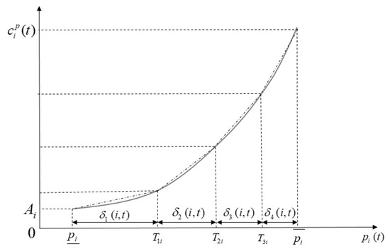
Figure 2. Piecewise linearization of cost curve.

The process of piecewise linearization of the cost curve can be expressed as the following formulas:

$$c_i^p(t)=A_i^{}{u}_i^t+{\displaystyle \sum _{l=1}^{L_i^{}}{F}_{l,i}^{}{\delta }_l^{}(i,t)}$$

(34)

$$p_i^{}(t)={\displaystyle \sum _{l=1}^{L_i^{}}{\delta }_l^{}(i,t)}+\underset{\_}{p_i^{}}{u}_i^t$$

(35)

$${\delta }_1^{}(i,t)\le T_{1,i}^{}-\underset{\_}{p_i^{}}$$

(36)

$${\delta }_l^{}(i,t)\le T_{l,i}^{}-T_{l-1,i}^{}$$

(37)

$${\delta }_{L_i^{}}^{}(i,t)\le \overline{p_i^{}}-T_{L_i^{}-1}^{},i$$

(38)

$${\delta }_l^{}(i,t)\ge 0$$

(39)

where $F_{l,i}$ is the increased cost of the i-th generator at the l section of the piecewise linearization curve, ${\delta }_l^{}(i,t)$ is the output of the i-th generator at the l section in moment t, and $L_i$ is the number of the piecewise section.

In the objective function, only the cost of CHP is nonlinear. Based on the piecewise linearization method above, the nonlinear constraint (Equation (13)) can be converted into Equation (40) as follows:

$$P_{CHP}^{g,t,s}=P_{CHP}^{g,\min }{u}_{CHP}^{g,t}+{\displaystyle \sum _{k=1}^{NK}{P}_{CHP}^{g,t,s,k}}$$

(40a)

$$F_{CHP}^{g,t,s}=F_{CHP}^{g,\min }{u}_{CHP}^{g,t}+{\displaystyle \sum _{k=1}^{NK}{P}_{CHP}^{g,t,s,k}{C}_{CHP}^{g,k}}$$

(40b)

Therefore, the objective function and constraints are linearized, and the problem can be converted into an MIP problem, solved using commercial solver CPLEX 12.4 (IBM, Armonk, NY, USA).

4. Results

4.1. Parameter and Settings

The developed model of a hybrid energy system was applied to a real demonstration project in China, which was conceptualized with representative costs and technical data from numerous previous studies. The hybrid energy system was composed of two photovoltaic modules, a wind turbine, two battery energy storage modules, four electric vehicle chargers, a combined heat and power, and a hydroelectric power plant, which is illustrated in detail in Table 2. The parameters of each module are represented in Table 3, Table 4, Table 5 and Table 6. The power outputs of renewable resources, including wind and PV and local load in a typical day, are represented in Figure 3. The time interval of RES is assumed as 15 min, and the period is 96. The electricity prices in a typical day are shown in Figure 4.

Table 2. Components of the hybrid energy system.

Module	Hydro	WG	PV	BESS	EV	CHP
Number	1	1	2	2	4	1
Installed capacity/kW	20,000	200	150,155	100	90	600

Table 3. Parameters of the hydro power.

Parameter	Value
Maximum output/kW	20,000
Minimum output/kW	500
Maximum capacity/Hm3	600
Minimum capacity/Hm3	200
Original capacity/Hm3	500
Final capacity/Hm3	500
Water flow/0.04 m3/s	0.04

Table 4. Parameters of combined heat and power (CHP).

Parameter	Value
Maximum output/kW	600
Minimum output/kW	60
Start-up cost/RMB	100
Maximum output of piecewise	200
Consumption coefficient of unit output	[0.6709,0.6934,0.7159]
Ramp-up rate/kW/min	600
Ramp-down rate/kW/min	600
heat-power ratio	2.54
Heat load/kJ	0

Table 5. Parameters of a battery energy storage system (BESS).

Parameter	Value
Discharging efficiency	0.9
Charging efficiency	0.9
Maximum SoC	160
Minimum SoC	40
Rated output	100
Depreciation expense of unit output/RMB	0.08
Original SoC	80
Final SoC	80

Table 6. Parameters of electric vehicle chargers (EV).

Parameter	Value
Rated power of charging pile/kW	90
Battery capacity of EV	324
Battery efficiency	0.08
Original quantity of EV	80
Final quantity of EV	80

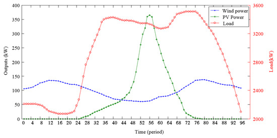
Figure 3. Output of renewable resources and load in a typical day.

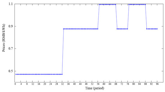
Figure 4. Electricity prices in a typical day.

Because of the influence of socioeconomic development and population growth, the demands can be described as parameters with a fluctuant interval. Hence, assume the fluctuating intervals of renewable resources and load demands as, respectively, ±20% and ±10% [39]. The confidence coefficient of risk is 0.95, and the risk aversion coefficient of the energy service provider is 0.3.

4.2. Results of the Proposed Model

Depending on the parameters above, construct 1500 scenes using Latin hypercube sampling, finally getting 150 scenarios with the scene reduction technology. Combined with the piecewise linearization method, the above proposed strategies are all MIP problems. Therefore, they can be solved by commercial solver CPLEX 12.4 efficiently, and the optimal results of the proposed model are shown in Table 7 and Table 8.

Table 7. Optimal output power of each generator in the above model.

Time	CHP/kW	BESS1/kW	BESS2/kW	EV1/kW	EV2/kW	EV3/kW	EV4/kW	Hydro/kW	Tie-Line Power/kW
1	0	0	0	0	0	54	0	0	2406
2	0	0	0	0	0	0	0	0	2352
3	0	0	0	0	0	0	0	0	2356
4	0	0	0	0	0	0	0	0	2364
5	0	0	0	0	54	0	0	0	2264
6	0	0	0	0	0	0	0	0	2210
7	0	0	0	0	0	0	0	0	2223
8	0	0	0	0	0	0	0	0	2236
9	0	0	0	54	0	0	0	0	2211
10	0	0	0	0	0	0	0	0	2103
11	0	0	0	0	0	0	0	0	2102
12	0	0	0	0	0	0	54	0	2114
13	0	0	0	0	0	0	0	0	2024.6
14	0	0	−29.63	0	0	0	0	0	2113.5
15	0	0	−29.63	0	0	0	0	0	2112.6
16	0	0	−29.63	0	0	0	0	0	2112.9
17	0	0	0	90	0	0	0	0	2156.7
18	0	0	0	0	90	0	0	0	2156.9
19	0	0	0	0	0	90	0	0	2157.2
20	0	0	0	0	0	0	90	0	2156.8
21	0	0	0	90	0	0	0	0	2185.8
22	0	0	0	0	90	0	0	0	2186.7
23	0	0	0	0	0	90	0	0	2186.3
24	0	0	0	0	0	0	90	0	2185.9
25	0	0	0	0	0	0	0	0	2485.89
26	0	−29.63	0	0	0	0	0	0	2575.7
27	0	−29.63	0	0	0	0	0	0	2576.4
28	0	−29.63	0	0	0	0	0	0	2577.9
29	15	0	0	0	90	0	0	0	3064.2
30	15	0	0	90	0	0	0	0	3065
31	15	0	0	0	0	0	90	0	3066.1
32	15	0	0	0	0	90	0	0	3065.7
33	150	0	0	0	0	0	0	125	3013.3
34	150	0	0	0	0	0	0	125	3013.5
35	150	0	0	0	0	0	0	125	3013.5
36	150	0	0	0	0	0	0	125	3015.1
37	150	0	0	0	0	0	0	1450	1721.2
38	150	0	0	0	0	0	0	1450.4	1713.4
39	150	0	0	0	0	0	0	1460.4	1701.6
40	150	0	0	0	0	0	0	1480	1678.2
41	150	0	0	0	0	0	0	3158	0
42	150	0	0	0	0	0	0	3158	0
43	150	0	0	0	0	0	0	3158	0
44	150	0	0	0	0	0	0	3158	0
45	150	0	0	0	0	0	0	125	2930
46	150	0	0	0	0	0	0	125	2929.1
47	150	0	0	0	0	0	0	125	2929.5
48	150	0	0	0	0	0	0	125	2931.2
49	150	0	0	0	0	0	0	125	2949.8
50	150	0	0	0	0	0	0	125	2950.1
51	150	0	0	0	0	0	0	125	2950.4
52	150	0	0	0	0	0	0	125	2951.2
53	150	0	0	0	0	0	0	3048	0
54	150	0	0	0	0	0	0	3050	0
55	150	0	0	0	0	0	0	3048	0
56	150	0	0	0	0	0	0	3048	0
57	150	0	0	0	0	0	0	3019	0
58	150	0	0	0	0	0	0	3019	0
59	150	0	0	0	0	0	0	3018.9	0
60	150	0	0	0	0	0	0	3019	0
61	150	0	0	0	0	0	0	3061	0
62	150	0	0	0	0	0	0	3060.5	0
63	150	0	0	0	0	0	0	3060.1	0
64	150	0	0	0	0	0	0	3061.2	0
65	150	0	0	0	0	0	0	3269.8	0
66	150	0	0	0	0	0	0	3270.1	0
67	150	0	0	0	0	0	0	3270.6	0
68	150	0	0	0	0	0	0	3270	0
69	150	0	0	0	0	0	0	125	3207.8
70	150	0	0	0	0	0	0	125	3207.7
71	150	0	0	0	0	0	0	125	3209.1
72	150	0	0	0	0	0	0	125	3211.4
73	150	0	0	0	0	0	0	125	3212.3
74	150	0	0	0	0	0	0	125	3213
75	150	0	0	0	0	0	0	125	3216
76	150	0	0	0	0	0	0	125	3210.5
77	150	0	18	0	0	0	0	3686.3	0
78	150	0	18	0	0	0	0	3686.3	0
79	150	0	18	0	0	0	0	3686.3	0
80	150	0	18	0	0	0	0	3687	0
81	150	0	0	0	0	0	0	3040	0
82	150	0	0	0	0	0	0	3041.8	0
83	150	0	0	0	0	0	0	3041.5	0
84	150	0	0	0	0	0	0	3039.7	0
85	150	0	0	0	0	0	0	2763.8	0
86	150	0	0	0	0	0	0	2765	0
87	150	0	0	0	0	0	0	2756.9	0
88	150	0	0	0	0	0	0	2764	0
89	150	0	0	0	0	0	0	125	2287.7
90	150	0	0	0	0	0	0	125	2284
91	150	0	0	0	0	0	0	125	2279.6
92	150	0	0	0	0	0	0	125	2290.1
93	150	36	0	0	0	0	0	2117	0
94	150	18	0	0	0	0	0	2117	0
95	150	18	0	0	0	0	0	2117	0
96	150	0	0	0	0	0	0	2117	0

Table 8. Optimal results of the proposed model.

	Cost/RMB	CVaR/RMB	Objective/RMB
Results	111,275	120,306	147,366

Table 7 represents the optimal output power of each generator in a hybrid energy system. Along with the increase of the local load demand, CHP and hydro power gradually begin to be put into operation, and the CHP operates at its maximum output all the time from the 33th period, while the output of hydro power changes with the fluctuation of the electricity price. Due to the electric vehicles needing a full charge to work before 8:00 a.m., the power exchange with EVs focuses on periods 1 to 32. With regard to the BESSs, they charge at a low electricity price between periods 14 to 16 and 26 to 28. and discharge at a high electricity price at 8:00 p.m. from periods 77 to 80 to get more economic benefits. From periods 53 to 68 and 77 to 88, the hydro power works at a high output power level because of the higher electricity price, while the tie-line power is zero to reduce the total cost in the hybrid energy system. Table 8 shows the optimal results of the proposed model in the hybrid system, consisting of the cost of operation and the cost of risk.

5. Discussion

In order to show the advantages of the proposed model, the tie-line power performance and the comparison results of the hybrid energy system with different situations are given in the following part, in which the effectiveness and the economy improvement are verified.

5.1. Comparison of Different Models

Considering the high cost of investment about BESS and charging piles, we compared the optimal results without the BESS or charging piles. The results of four different models are shown in Table 9. The tie-line power with power grid is represented in Figure 5.

Table 9. Optimal results of the compared models.

	Include All	No BESS	No EV	No BESS and EV
Cost/RMB	111,275	111,291	110,664	110,680
CVaR/RMB	120,306	120,324	119,693	119,710
Objective/RMB	147,366	147,388	146,572	146,593

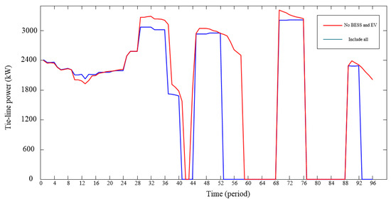
Figure 5. Tie-line power of the compared model.

BESS has the ability to store energy, so it can discharge at high prices and charge at a low price to reduce the economic cost and stabilize the tie-line power. Comparing scheduling models where BESS participates and where it does not, we found that the total cost and risk all dropped, and the economic objective was lower in Table 9, which is consistent with the fact. Regarding the hybrid energy system, the charging piles of EV are opposite to the BESS. The charging piles can be seen as a controllable load, so the total cost and risk will drop without them.

Figure 5 shows the tie-line power curve of the compared model. Throughout the time of operation, the curve of the model including all is much smoother than the compared model without BESS and EV. At periods 28 to 42, 46 to 59, and 70 to 76, the power of the tie-line in the proposed model is lower than those of the compared models without BESS and EV, respectively. Therefore, with the diversification of load demands, expanding the types of energy is important to peak shaving and valley filling.

In order to show the advantages of the proposed method, the computational time and the comparison results of the hybrid energy system with different situations are given in the following part.

5.2. Comparison of Different Methods

It is important to compare the proposed method with traditional methods regarding the above model, including all energy modules. This paper illustrates and compares the following three cases to investigate the advantages of the proposed method. Case 1 is the method proposed in this paper, and case 2 is the method with Monte Carlo sampling, scene reduction, and piecewise linearization. Case 3 is the intelligent method (PSO). The results of the three different methods are shown in Table 10.

Table 10. Optimal results of the compared methods.

	Objective/RMB	Computational Time/s
Case 1 (PL-LHSSR)	147,366	23.38
Case 2 (PL-MCSR)	147,371	25.14
Case 3 (PSO)	147,366.8	80.02

The method in case 2 is similar to the proposed method in case 1, and the difference is the sampling method. In Table 10, the results of the objective and computational time in case 2 is slightly more than those in case 1. However, the computational time of the intelligent method (PSO) is much longer than that in case 1. The computational time in case 3 is nearly four times as long as that in case 1. The main reason is that piecewise linearization can effectively reduce the solving time. The objective result in case 3 is slightly equal to case 2. From Table 10, the proposed method has advantages in optimal results and computational time.

5.3. Impact of the Fluctuation of Uncertainty Variables

According to different seasons and regions, the difference of load curve and renewable resources is obvious. Therefore, it is necessary to consider the fluctuation of uncertainty variables on the influence of the objective function. Considering three scenarios: Reduction of 10%, unchanged, and increase of 10%, the optimal results are shown as follows:

Table 11 represents the effects of the fluctuation of uncertainty variables on the objective function of the proposed model in hybrid energy system. Wind and PV as renewable resources have the features of low cost and high risk. With the increasing output of wind or PV, the cost reduces from 111,275 to 111,114 and 111,135, while the risk increases from 120,306 to 120,471 and 120,429 in Table 11. The results are opposite as to the case of decreasing output. In addition, the fluctuation of local load results has much more of an impact on the optimal results. The relative change reaches 20% when the load fluctuates by 10%, while the relative change only reaches 1% when the renewable resources fluctuate by 10%. Therefore, it is particularly important to improve the forecasting accuracy of the load demand.

Table 11. Optimal results of the uncertainty fluctuations.

Results	Cost/RMB	CVaR/RMB	Objective/RMB
Initial	111,275	120,306	147,366
Wind + 10%	111,114	120,471	147,255
Wind − 10%	111,436	120,140	147,478
PV + 10%	111,135	120,429	147,264
PV − 10%	111,414	120,183	147,469
Load + 10%	132,794	142,718	175,609
Load − 10%	89,755	97,891	119,122

5.4. Impact of the Time Intervals of RES

According to different granularity requirements, the difference in time intervals of RES is obvious. Therefore, it is necessary to consider the different granularity requirements of RES on the influence of the objective function. Considering three scenarios: 5-min intervals, 10-min intervals, and 15-min intervals, the optimal results are shown as follows:

Table 12 represents the sensitive studies of different time intervals of RES. Due to the small scale of RES compared to the whole scale of energy system, the impact of different time intervals on the optimal results can be negligible. The objective results of different scenarios are approximately equal.

Table 12. Optimal results of different time intervals.

Results	Cost/RMB	CVaR/RMB	Objective/RMB
5-min	111,275	120,303	147,365
10-min	111,275	120,306	147,366
15-min	111,275	120,306	147,366

5.5. Impact of the Coefficient of Risk Aversion

In the renewable-based hybrid energy system supplied by energy service providers, different providers have different coefficients of risk aversion. Consider five scenarios to study the impact of risk coefficient for optimization model. The optimal results are shown in Table 13.

Table 13. Components of the hybrid energy system.

Coefficient of Risk Aversion	Objective/RMB
0.1	123,301
0.2	135,335
0.3	147,366
0.5	171,423
0.8	207,519

Table 13 represents the sensitive studies on the provider’s risk aversion for the hybrid energy system. A larger coefficient of risk aversion for the energy service provider indicates less tolerance towards possible uncertainty in the model. With the increase of the coefficient of risk aversion, the system pays more attention to risk, leading to the increase in the cost of risk. Thus, the hybrid system’s objective cost is increased by the increase in coefficient of risk aversion.

6. Conclusions

This paper proposed a concept of a renewable-based hybrid energy system which can effectively restrain the fluctuations in wind and photovoltaic generation to improve their stabilities. Taking into account the cost of operation and risk, an optimal scheduling model of this system was put forward. An optimization method was proposed based on Latin hypercube sampling, scene reduction, and piecewise linearization. The main achievements and conclusions are listed below:

(1)

A concept of a renewable-based hybrid energy system including PV, WT, BESS, EV, CHP, and hydroelectric power was proposed to solve the reliable and economically justifiable integration of RES into the power system.

(2)

An optimal scheduling model of this system was put forward considering the cost of operation and risk.

(3)

An optimization method was proposed based on Latin hypercube sampling, scene reduction, and piecewise linearization to deal with multiple uncertainties, including renewable resource volatility, the load demand, and different energy service providers’ coefficient of risk aversion.

(4)

Based on the real data obtained in China, the performance of the proposed model and method was evaluated. Results showed that the renewable-based hybrid system can not only reduce the intermittent and volatility of renewable resources but also ensure the smoothness of the tie-line power as much as possible. The effectiveness and the economy improvement of the proposed model and method were verified.

(5)

In future studies, the environmental factors of the hybrid energy system and how to deal with uncertainty efficiently in a power system can be studied. Hence, how to improve the reliable and economically justifiable integration of RES into the power system is worth further research.

References

- Wang, L.; Vo, Q.; Prokhorov, A.V. Stability Improvement of a Multimachine Power System Connected with a Large-Scale Hybrid Wind-Photovoltaic Farm Using a Supercapacitor. IEEE Trans. Ind. Appl. 2018, 54, 50–60. [Google Scholar] [CrossRef]
- Fabbri, A.; Roman, T.G.S.; Abbad, J.R.; Quezada, V.M. Assessment of the cost associated with wind generation prediction errors in a liberalized electricity market. IEEE Trans. Power Syst. 2005, 20, 1440–1446. [Google Scholar] [CrossRef]
- Jurasz, J.; Mikulik, J.; Krzywda, M.; Ciapała, B.; Janowski, M. Integrating a wind-and solar-powered hybrid to the power system by coupling it with a hydroelectric power station with pumping installation. Energy 2018, 144, 549–563. [Google Scholar] [CrossRef]
- Liserre, M.; Sauter, T.; Hung, J.Y. Future energy systems: Integrating renewable energy sources into the smart power grid through industrial electronics. IEEE Ind. Electron. Mag. 2010, 4, 18–37. [Google Scholar] [CrossRef]
- Jones, L.E. Renewable Energy Integration: Practical Management of Variability, Uncertainty, and Flexibility in Power Grids; Academic Press: Cambridge, MA, USA, 2014. [Google Scholar]
- Mwasilu, F.; Justo, J.J.; Kim, E.K.; Do, T.D.; Jung, J.W. Electric vehicles and smart grid interaction: A review on vehicle to grid and renewable energy sources integration. Renew. Sustain. Energy Rev. 2014, 34, 501–516. [Google Scholar] [CrossRef]
- Papaefthymiou, S.V.; Karamanou, E.G.; Papathanassiou, S.A.; Papadopoulos, M.P. A wind-hydro-pumped storage station leading to high RES penetration in the autonomous island system of Ikaria. IEEE Trans. Sustain. Energy 2010, 1, 163–172. [Google Scholar] [CrossRef]
- Wang, K.Y.; Luo, X.J.; Wu, L.; Liu, X.C. Optimal coordination of wind-hydro-thermal based on water complementing wind. Renew. Energy 2013, 60, 169–178. [Google Scholar] [CrossRef]
- Malakar, T.; Goswami, S.K.; Sinha, A.K. Impact of load management on the energy management strategy of a wind-short hydro hybrid system in frequency based pricing. Energy Convers. Manag. 2014, 79, 200–212. [Google Scholar] [CrossRef]
- Kellogg, W.D.; Nehrir, M.H.; Venkataramanan, G.; Gerez, V. Generation unit sizing and cost analysis for stand-alone wind, photovoltaic, and hybrid wind/PV systems. IEEE Trans. Energy Convers. 1998, 13, 70–75. [Google Scholar] [CrossRef]
- De Almeida, A.T.; Martins, A.; Jesus, H.; Climaco, J. Source reliability in a combined wind-solar-hydro system. IEEE Trans. Power Appar. Syst. 1983, 6, 1515–1520. [Google Scholar] [CrossRef]
- Reddy, S.S. Optimal scheduling of thermal-wind-solar power system with storage. Renew. Energy 2017, 101, 1357–1368. [Google Scholar] [CrossRef]
- Biswas, P.P.; Suganthan, P.N.; Amaratunga, G.A.J. Optimal power flow solutions incorporating stochastic wind and solar power. Energy Convers. Manag. 2017, 148, 1194–1207. [Google Scholar] [CrossRef]
- Moghaddam, I.G.; Nick, M.; Fallahi, F.; Sanei, M.; Mortazavi, S. Risk-averse profit-based optimal operation strategy of a combined wind farm–cascade hydro system in an electricity market. Renew. Energy 2013, 55, 252–259. [Google Scholar] [CrossRef]
- Khodayar, M.E.; Abreu, L.; Shahidehpour, M. Transmission-constrained intrahour coordination of wind and pumped-storage hydro units. IET Gener. Transm. Distrib. 2013, 7, 755–765. [Google Scholar] [CrossRef]
- Helseth, A.; Gjelsvik, A.; Mo, B.; Linnet, Ú. A model for optimal scheduling of hydro thermal systems including pumped-storage and wind power. IET Gener. Transm. Distrib. 2013, 7, 1426–1434. [Google Scholar] [CrossRef]
- De la Nieta, A.A.S.; Contreras, J.; Muoz, J.I.; Catalo, J.P. Optimal wind reversible hydro offering strategies for midterm planning. IEEE Trans. Sustain. Energy 2015, 6, 1356–1366. [Google Scholar] [CrossRef]
- Meibom, P.; Hilger, K.B.; Madsen, H.; Vinther, D. Energy comes together in Denmark: The key to a future fossil-free Danish power system. IEEE Power Energy Mag. 2013, 11, 46–55. [Google Scholar] [CrossRef]
- Benam, M.R.; Madani, S.S.; Alavi, S.M.; Ehsan, M. Optimal configuration of the CHP system using stochastic programming. IEEE Trans. Power Deliv. 2015, 30, 1048–1056. [Google Scholar] [CrossRef]
- Sheikhi, A.; Ranjbar, A.M.; Oraee, H. Financial analysis and optimal size and operation for a multicarrier energy system. Energy Build. 2012, 48, 71–78. [Google Scholar] [CrossRef]
- Freschi, F.; Giaccone, L.; Lazzeroni, P.; Repetto, M. Economic and environmental analysis of a trigeneration system for food-industry: A case study. Appl. Energy 2013, 107, 157–172. [Google Scholar] [CrossRef]
- Fumo, N.; Mago, P.J.; Chamra, L.M. Emission operational strategy for combined cooling, heating, and power systems. Appl. Energy 2009, 86, 2344–2350. [Google Scholar] [CrossRef]
- Wang, J.J.; Jing, Y.Y.; Zhang, C.F. Optimization of capacity and operation for CCHP system by genetic algorithm. Appl. Energy 2010, 87, 1325–1335. [Google Scholar] [CrossRef]
- Ren, H.; Gao, W.; Ruan, Y. Optimal sizing for residential CHP system. Appl. Therm. Eng. 2008, 28, 514–523. [Google Scholar] [CrossRef]
- Aringhieri, R.; Malucelli, F. Optimal operations management and network planning of a district heating system with a combined heat and power plant. Ann. Oper. Res. 2003, 120, 173–199. [Google Scholar] [CrossRef]
- Rolfsman, B. Combined heat-and-power plants and district heating in a deregulated electricity market. Appl. Energy 2004, 78, 37–52. [Google Scholar] [CrossRef]
- Zugno, M.; Morales, J.M.; Madsen, H. Robust management of combined heat and power systems via linear decision rules. In Proceedings of the 2014 IEEE International Energy Conference (ENERGYCON), Cavtat, Croatia, 13–16 May 2014; pp. 479–486. [Google Scholar]
- Dimoulkas, I.; Amelin, M. Constructing bidding curves for a CHP producer in day-ahead electricity markets. In Proceedings of the 2014 IEEE International Energy Conference (ENERGYCON), Cavtat, Croatia, 13–16 May 2014; pp. 487–494. [Google Scholar]
- De Ridder, F.; Claessens, B. A trading strategy for industrial CHPs on multiple power markets. Int. Trans. Electr. Energy Syst. 2014, 24, 677–697. [Google Scholar] [CrossRef]
- Lahdelma, R.; Hakonen, H. An efficient linear programming algorithm for combined heat and power production. Eur. J. Oper. Res. 2003, 148, 141–151. [Google Scholar] [CrossRef]
- Rao, P.S.N. Combined heat and power economic dispatch: A direct solution. Electr. Power Compon. Syst. 2006, 34, 1043–1056. [Google Scholar] [CrossRef]
- Salgado, F.; Pedrero, P. Short-term operation planning on cogeneration systems: A survey. Electr. Power Syst. Res. 2008, 78, 835–848. [Google Scholar] [CrossRef]
- Lai, S.M.; Hui, C.W. Integration of trigeneration system and thermal storage under demand uncertainties. Appl. Energy 2010, 87, 2868–2880. [Google Scholar] [CrossRef]
- Carpaneto, E.; Chicco, G.; Mancarella, P.; Russo, A. Cogeneration planning under uncertainty. Part II: Decision theory-based assessment of planning alternatives. Appl. Energy 2011, 88, 1075–1083. [Google Scholar] [CrossRef]
- Zapata, J.; Vandewalle, J.; D’haeseleer, W. A comparative study of imbalance reduction strategies for virtual power plant operation. Appl. Therm. Eng. 2014, 71, 847–857. [Google Scholar] [CrossRef]
- Liao, J.; Chuang, Y.; Yang, H.; Tsai, M. BESS-Sizing Optimization for Solar PV System Integration in Distribution Grid. IFAC-Pap. Online 2018, 51, 85–90. [Google Scholar] [CrossRef]
- Chettibi, N.; Mellit, A. Intelligent control strategy for a grid connected PV/SOFC/BESS energy generation system. Energy 2018, 147, 239–262. [Google Scholar] [CrossRef]
- Branco, H.; Castro, R.; Lopes, A.S. Battery energy storage systems as a way to integrate renewable energy in small isolated power systems. Energy Sustain. Dev. 2018, 43, 90–99. [Google Scholar] [CrossRef]
- Li, G.; Sun, W.; Huang, G.H.; Lv, Y.; Liu, Z.; An, C. Planning of integrated energy-environment systems under dual interval uncertainties. Int. J. Electr. Power Energy Syst. 2018, 100, 287–298. [Google Scholar] [CrossRef]
© 2019 by the authors. Licensee MDPI, Basel, Switzerland. This article is an open access article distributed under the terms and conditions of the Creative Commons Attribution (CC BY) license (http://creativecommons.org/licenses/by/4.0/).