Abstract
Urbanization is an important factor in the growth of carbon emissions, as the city is a dense area of carbon emissions. This paper estimates the carbon emissions at the provincial, municipal, and county spatial scales in the Yangtze River Delta region during 2008–2015. On this basis, this paper makes a comprehensive analysis of the pathway and difference of the urbanization to the carbon emission by using the scale variance decomposition method, the space correlation analysis method, the mediation effect test method, and the space panel data model. The results show that the urbanization of the Yangtze River Delta has a significant positive impact on carbon emissions; The pathway from urbanization to industrial structure has a significant impact on carbon emissions. Although the pathway from industrial structure to urbanization to carbon emissions is insignificant, the industrial structure directly affects carbon emissions. There is a significant path from urbanization to the level of economic development to carbon emissions, but there is no mechanism for the economic development level to adversely affect the level of urbanization and thus affect carbon emissions; the chain action pathway from the urbanization level to the employment level to the economic development level to carbon emissions is not significant. Finally, based on the research conclusions, the corresponding policy recommendations are submitted.
1. Introduction
With the in-depth implementation of the new urbanization strategy, China’s urbanization has entered a stage of rapid development. The urbanization rate reached 53.73% in 2013, which is close to the world average level, while there are still some gaps when compared with the developed countries with about 80% urbanization rate. The rapid acceleration of urbanization has caused increasingly serious ecological problems. As the world’s largest carbon emitter, China has an inescapable responsibility in reducing carbon emissions [1]. To this end, the Chinese government has solemnly promised: by 2020, China’s carbon emissions will be 40% to 45% lower than in 2005. This is also the responsibility of China as a responsible big country. Studying carbon emissions from the perspective of urbanization is not only conducive to the coordinated development of China’s economy, population, resources, and environment, but it is also conducive to the scientific formulation of carbon emission reduction policies and the smooth realization of carbon emission reduction targets. Therefore, exploring the impact of urbanization on carbon emissions has important practical and theoretical implications. In view of this, this paper will locate the research area in the Yangtze River Delta urban agglomeration (all the administrative areas of Shanghai, Zhejiang, and Jiangsu, the specific situation is shown in Figure 1) and analyze how the path and difference in regional urbanization development affect carbon emissions, with a view of providing reference for China’s new urbanization development and carbon emission reduction targets.
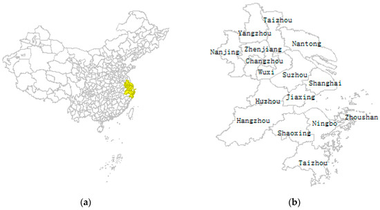
Figure 1.
Location and area map of the Yangtze River Delta. (a) Location map of the Yangtze River Delta and (b) Map of the Yangtze River Delta.
Existing studies generally believe that the level of urbanization has an important impact on regional carbon emissions [2,3]. Some scholars found that "a linear relationship between urbanization and carbon emissions" [4,5], while some scholars believe that "the direct relationship, between urbanization and carbon emissions, is not just a simple linear relationship. Urbanization has both driving and braking effects on carbon emissions” [6,7,8]. When urbanization is in its infancy, the population of urban areas is growing rapidly. The proportion of the primary industry has gradually declined, the proportion of the secondary and tertiary industries has gradually increased, and people’s lifestyles are also gradually becoming more carbonized [9,10,11]. At this time, the scale and the agglomeration effects of the towns have not yet formed, and the combination of these factors, the driving effect of urbanization on carbon emissions, is greater than that of the braking effect, which is reflected in the positive effect of urbanization on carbon emissions [12,13,14]. However, when urbanization develops to a certain level, the scale and agglomeration effects of urbanization and the effect of technology diffusion gradually appear. Together, these factors cause the braking effect of urbanization on carbon emissions to be greater than the driving effect, which is manifested in the negative impact of urbanization on carbon emissions. [15,16,17,18]. Some scholars, such as Asumadu Sarkodie and Phebe Asantewaa Owus. [19], believe that the impact of urbanization on carbon emissions is insignificant.
With the deepening of research, some scholars have gradually realized that there are still major obstacles to establish a clear and direct link between urbanization and carbon emissions. Because the impact of urbanization on carbon emissions is a complex issue that involves many levels, many other factors also impact on carbon emissions, which is the result of the combination of urbanization and other factors. Accordingly, most of the studies have combined urbanization with other relevant factors to examine its impact on carbon emissions—the combined effect. In the joint effect analysis, different scholars selected different impact factors according to the spatial scale of the study and the research purpose, but these generally included the population size, population density, or spatial distribution of population, economic scale, and industrial structure. From the overall research results, it is generally believed that urbanization, related variables, and carbon emissions have a long-term equilibrium relationship [20,21]. However, the research results of specific indicators have different conclusions, because of differences in the scales of research, methods, and factors that were included in the model [22].
Although a great deal of literature has strongly demonstrated the strong correlation between urbanization, related factors, and carbon emissions, many meaningful conclusions and inspirations have been obtained. However, the mechanism of urbanization affecting carbon emissions is extremely complicated. On the one hand, urbanization is more indirectly affected by carbon emissions through other factors, such as production and living [23]. The advancement of urbanization has caused the population to continue to gather in urban areas. Large-scale infrastructure construction, such as roads and buildings in urban areas, will generate a large amount of carbon emissions during the construction process and in the future [24], while urbanization is also a process in which the working population flows from the primary industry to the secondary and tertiary industries. For the primary industry, the decrease in the number of primary industry practitioners promotes a significant increase in the logistics activities that are related to the transportation of agricultural products, and to a certain extent it also promotes the mechanization of the primary industry, thereby increasing carbon emissions. For the secondary and tertiary industries, the concentration of population factors has prompted rapid development, while the high-energy consumption production methods of the secondary and tertiary industries increase carbon emissions [25,26,27,28]. In addition, the promotion of urbanization also accelerates the development of fixed assets investment, cement, export trade, and other industries, which indirectly promotes the growth of carbon emissions. On the other hand, there is a strong correlation between land use, industrial expansion, and carbon emissions. Land use and industrial expansion have a stable contribution to economic growth, and the intensive use of land is gradually increasing with the advancement of science and technology [29]. However, a large amount of greenhouse gases are generated in the process of land use [30,31], which indirectly increase carbon emissions.
Throughout the above studies, it can be observed that the current research on the relationship between urbanization and carbon emissions mainly focuses on the study of the total effect (such as X→Y) and direct effect (such as X + M1 + M2→Y), but this is only a part of the mechanism of urbanization-driven carbon emissions, and it is a very important way for urbanization to act on carbon emissions; that is, indirect research (indirect or mediating effects, such as X→M1→Y; X→M2→Y; X→M1→M2→Y) are not enough. Ignoring the specific roles of other factors in this process often makes the interpretation of statistical results ambiguous and it may lead to the wrong conclusions. In terms of research methods, the current research mainly uses traditional econometric study methods, and it ignores the spatial correlation of carbon emissions between regions. Based on this, this paper study the role of urbanization development of the Yangtze River Delta urban agglomeration on carbon emissions on the basis of spatial correlation.
2. Methodology and Data
Figure 2 shows the method flow chart of this paper.
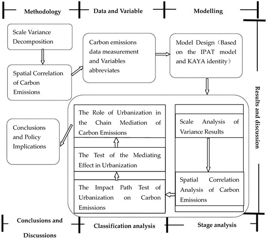
Figure 2.
A flow chart of methodology.
2.1. Methodology
2.1.1. Scale Variance Decomposition
The scale analysis of variance can quantitatively analyze the economic differences at different spatial scales in the region to identify the optimal spatial scale, so it has been widely used in multi-space scale analysis [32,33]. Therefore, this paper uses the scale variance decomposition method to study the carbon emissions in the Yangtze River Delta region and to identify the optimal spatial scale.
The scale variance analysis method first needs to divide the research area into different levels of spatial hierarchy and layer the research units of different scales according to certain criteria. According to the administrative division, the Yangtze River Delta region is divided into three spatial scales and the county scale is the minimum spatial scale. The regional nesting includes the city scale according to the provincial scale, the city scale includes the county scale standard, and the three levels of spatial scale, defined as the provincial, municipal, and county domains, are represented by α, β, and γ respectively, and they indicate that the statistical model of the variance within the region is as follows.
represents the carbon emissions of the (k)th county in the (j)th city of the (i)th province and , , , , and , . N represents the number of counties in the Yangtze River Delta; indicates the number of counties in the (i)th province; and indicates the number of counties in the (j)th city of the (i)th province. Table 1 shows the composition of the scale variance at different spatial scales.

Table 1.
Scale variance composition at different scales.
2.1.2. Spatial Correlation of Carbon Emissions
There are similarities between economic environment or geographical environment in geographically adjacent areas. These factors may cause the regional carbon emissions to show certain correlations, that is, spatial correlations. Moran’s I statistical variable is widely used as a measure of the spatial correlations between inter-regional economic variables. Indeed, the addition of local Anselin and Gestis-Ord hot spot analysis can more fully demonstrate the spatial characteristics of carbon emissions, because this part is not the focus of this paper, this part is not included in the text. The Moran’s I formula is as follows.
, indicates the amount of carbon emissions in region i; n is the number of regions; and, W represents the spatial weight matrix. Its value range between -1 and 1. The closer that the value of I is to 1, the stronger the positive spatial correlation of the carbon emissions between the regions is, I values closer to −1, indicated stronger negative spatial correlations of carbon emissions between the regions, while those that are closer to zero indicates that there is no spatial correlation between carbon emissions.
When measuring the spatial correlation of a region, it is first necessary to define a spatial weight matrix to describe the spatial neighbor relationship. The spatial weight matrix is generally divided into the adjacent spatial weight matrix, the geographic distance spatial weight matrix, and the economic distance spatial weight matrix. In the geographic distance spatial weight matrix, determining the Euclidean distance between two points is necessary. Therefore, the spatial distance weight matrix is not considered in the modeling analysis.
The adjacent spatial weight matrix is mainly used to describe the geographic border relationship of regions, and it is an important weight matrix for describing relative positional relationships. In this paper, we use the first-order car adjacent to define the adjacent spatial weight matrix, as shown in Equation (3):
The economic distance spatial weight matrix is used to describe the difference in economic development level between the two regions. It is a weight matrix that describes the absolute positional relationship between the regions from an economic perspective. The formula is as shown in Equation (4):
represents the economic development of region I; it is usually measured by Gross Domestic Product (GDP). This paper uses the real GDP average values from 2008 to 2015 (based on 2008), which eliminated the factor of inflation.
2.2. Data
2.2.1. Carbon Emissions Data Measurement
This paper selects coal, coke, crude oil, gasoline, kerosene, diesel, fuel oil, and natural gas to calculate carbon emissions. The calculation formula for carbon emissions is as follows:
Standard coal represents the consumption of the (j)th energy in the (i)th region, and it is obtained by multiplying the consumption of the energy by the standard coal conversion coefficient. The various energy conversion factors are taken from the China Energy Statistical Yearbook. indicates the carbon emission coefficient of this energy source. The specific value is derived from the Intergovernmental Panel on Climate Change (IPCC)’s National Greenhouse Gas Emission Inventory Guide 2006. The standard coal conversion coefficient and the carbon emission coefficient are shown in Table 2.
Table 2.
The value of the energy conversion standard coal coefficient and carbon emission coefficient.
All of the data in this paper are from China Statistical Yearbook, China Energy Statistical Yearbook, and City Statistical Yearbook of the Yangtze River Delta from 2009 to 2016. The urbanization data of some counties (county-level cities) are missing. In order to ensure statistical consistency, this paper characterizes the level of urbanization according to the proportion of the non-agricultural population at the end of the year.
2.2.2. Variables abbreviates
The Table 3 is an explanation of the abbreviations of the variables that appear in the text.
Table 3.
The explanation of variables.
2.3. Model Design
Most scholars [34,35,36] often use two basic conceptual models to study the factors that affect carbon emissions: the IPAT (Environmental load, Population, Affuence, Technology)model and KAYA identity (First proposed by Japanese professor Yoichi Kaya at a seminar of IPCC in 1989, decomposes carbon emissions into four influencing factors).
IPAT model is created by a well-known demographer Professor Paul R. Ehrlich of Stanford University in the United States, who proposed an identical equation regarding the relationship between environmental load (I) and population (P), affluence (A), and technology (T):
Formula (6) indicates the pressure of economic development on resources and environment, P indicates the total population, A indicates the level of per capita resource consumption or consumption (per capita GDP), T indicates the degree of environmental damage that is caused by various technologies providing consumer goods, which is also known as environmental efficiency, as expressed in material terms.
The KAYA identity decomposes carbon emissions into four influencing factors. The formula is as follows:
P indicates the population size, G indicates the gross national product (GDP), E indicates the energy consumption, G/P indicates the per capita GDP, E/G indicates the energy consumption intensity, and C/E indicates the energy consumption carbon intensity.
Referring to these two conceptual models, based on the basic principles of economics and previous research conclusions [37,38], this paper extracts the theoretical path of urbanization on carbon emissions.
① Urbanization → The proportion of secondary industry → Carbon emissions
② Urbanization → The proportion of tertiary industry → Carbon emissions
③ The proportion of secondary industry → Urbanization → Carbon emissions
④ The proportion of tertiary industry → Urbanization → Carbon emissions
⑤ Urbanization → Economic development level → Carbon emissions
⑥ Economic development level → Urbanization → Carbon emissions
⑦ Urbanization → Social Employment Level → Economic Development Level → Carbon Emissions
The STIRPAT model is the basic model for decomposing carbon emissions. The specific form is as shown in Equation (8).
represents a random error term. By taking the natural logarithm of both sides of the formula (8), the equation can be transformed into a linear model, which facilitates the estimation of the model and the addition of other influencing factors. This paper explores the mechanism of action of various factors on carbon emissions that are based on the STIRPAT model.
According to the previous analysis, carbon emissions have a positive spatial correlation under the economic distance spatial weight matrix, so the spatial correlation between regions should be considered when constructing the empirical model. Based on this, this paper establishes a spatial panel model with both time and space effects that are based on the STIRPAT model. The specific form of the model is as shown in Equation (9).
i, j represents different regions; represents the economic distance spatial weight matrix; represents the independent variable vector; represents the carbon emissions; is the independent variable regression coefficient vector; is the dependent variable spatial regression coefficient; φ is the independent variable spatial regression coefficient; and λ is the spatial error regression coefficient.
If , , then Equation (9) is a spatial lag panel data model (SLPDM) that measures the impact of carbon emissions in the adjacent regions on carbon emissions in a local region. If , , then Equation (9) is a spatial error panel data model (SEPDM) that reflects the influence of factors that have not been considered, except for independent variables in adjacent regions on carbon emissions. If , , , then Equation (9) is a spatial Durbin panel data model (SDPDM) that measures both the carbon emissions in adjacent areas and the influence of neighbouring areas’ independent variables on carbon emissions in the local area.
In the course of the research, the LR (Likelihood Ratio)and Wald (Wald test was proposed by Wald in 1943) tests are generally used to determine which form of spatial panel model to use. The specific test steps are as follows: (1) establish a spatial Durbin panel data model (SDPDM) and estimate it; (2) propose two null hypotheses (: the spatial Durbin panel data model can be simplified to the spatial lag panel data model (SLPDM); and, : the spatial Durbin panel model can be simplified to the spatial error panel data model (SLPDM)); and, (3) the significance level of the two hypotheses is measured. It is assumed that the rejection of the two hypotheses at the same time would cause the establishment of the spatial Durbin panel data model.
First, the model was tested by LR, Wald, and Hausman. The test results are shown in Table 4.
Table 4.
The results of LR, Wald, and Hausman tests in the spatial panel data model.
It can be seen from the test results in Table 4 that the null hypothesis of the Hausman test is rejected when the significance level is 1%. At the same time, the spatial lag model of LR test and Wald test are significant when the significance level is 1%, the spatial error model of LR test and Wald test are significant when the significance level is 1%, so it is determined that the spatial effect of the fixed-effect spatial Durbin panel data model should be used in modeling analysis.
The median effect test method is widely used in the field of psychology. It can be used to analyze the influence and transmission mechanism between variables. Therefore, in recent years it has been widely used in the fields of medicine, economics, and management.
The dependent variable is set as X, the mediating variable is M, and the dependent variable is Y. The following test models are separately constructed.
represents the carbon emissions; represents the independent variable vector, that is, , , and represent the regression residual terms. c represents the total effect, a, b represents the mediating effect, and c’ represents the direct effect.
In this paper, the stepwise regression method is used to test the mediating effect. The test steps are as follows: (1) we determined whether the test coefficient c is significant, if it is then we proceed to the next step; (2) we check whether the coefficients a, b is significant. If they are significant, we test the coefficient c’. If at least one coefficient is not significant, the sobel test is performed. If it is significant, this indicates that the mediation effect is outstanding. If it is not significant, then this indicates that the mediation effect is not remarkable. (3) If the coefficient c’ is significant, it indicates that there is a portion mediating effect. If it is not significant, this indicates that there is a complete mediating effect.
3. Results and Analysis
3.1. Scale Analysis of Variance Results
The carbon emissions at different spatial scales are scaled according to the formula of Table 1. The results of the variance analysis are shown in Figure 3.
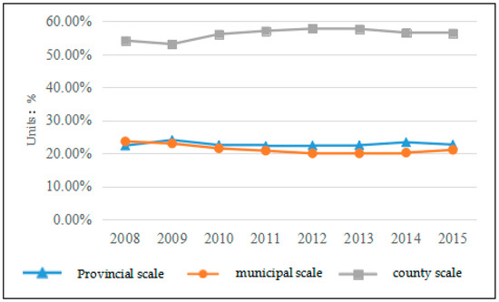
Figure 3.
Scale variance decomposition of different scales of the Yangtze River Delta in 2008–2015.
The results of the scale analysis of variance show that from 2008 to 2015, at the county level, carbon emissions carry the largest amount of information, and their contribution rate is higher than those of the provincial and municipal scales, accounting for more than 50% of the total information, on average. The contributions of the provincial and municipal scales have remained at a level of 23%.
From the perspective of scale variance, as is consistent with previous studies [39], the roles of urbanization and mediating variables on carbon emissions at the county scale reflect the overall level of force in the Yangtze River Delta relatively more objectively, but it is clear that there are no advantages or disadvantages at various scales. In order to study the economic phenomena at the spatial scale, it is necessary to construct a model on the spatial scale.
3.2. Spatial Correlation Analysis of Carbon Emissions
The estimated results of Table 5 are consistent with those of previous studies, indicating that there are spatial effects on carbon emissions in cities in the Yangtze River Delta [40], but the difference is that the carbon emissions in the Yangtze River Delta show significant positive spatial correlation under the economic distance spatial weight matrix. Under the adjacent spatial weight matrix, the carbon emissions of the Yangtze River Delta show negative spatial correlation, but at the 10% significance level, this negative spatial correlation is not significant. In regard to the economic distance and space weight, at the 5% significance level there is a positive spatial correlation between carbon emissions in areas of similar economic development. From this, it can be judged that the geographical proximity is not the main reason for the spatial correlation of carbon emissions in the Yangtze River Delta. This may be because different city-level units use administrative orders to lay out the industry. At junctions between cities, there is often a county with high carbon emissions holding another county with low carbon emissions. This phenomenon is particularly common in the Jiangsu province. For the purpose of protecting the environment of this city, some cities have placed high-energy consumption and high-pollution enterprises in county areas where the city’s winter winds travel towards, and for neighboring cities, the county in this position is the central city. The administrative units do not deploy high-pollution and high-energy-consuming enterprises in the upward direction, which results in a negative spatial correlation of carbon emissions in geographically adjacent areas. The reason why this negative spatial correlation is not significant may be that the administrative boundaries of different urban areas have became blurred at the county scale.
Table 5.
Moran’s value of carbon emissions from the county scale under the two-weight matrix.
The carbon emissions in the Yangtze River Delta show a significant positive spatial correlation under the economic distance spatial weight matrix. This shows that the areas with similar economic development levels have similar carbon emissions. The reason for this is that the areas with similar levels of economic development have mutual learning and mutual influence during the process of urbanization, industrial planning, and economic development planning.
3.3. The Impact Path Test of Urbanization on Carbon Emissions
From Table 6, we can see the following.
Table 6.
Impact path test result of Urbanization → Mediating Variables → Carbon Emissions.
(1) The total benefits and direct effects of urbanization on carbon emissions.
From the estimation results of Column1, Column4, and Column7 in Table 6, the urbanization level (lnU) coefficient is statistically significant at the 5% significance level, indicating that the total effect of lnU on carbon emissions (lnY) is significant. From the results of Column3, Column6, and Column9, the lnU coefficients are statistically significant at the 5% significance level, indicating that the direct effect of lnU on lnY is significant. Moreover, lnU has a positive impact on lnY, different from previous studies [32], indicating that the scale effect of urbanization on carbon emissions has not yet appeared. This is mainly because the overall urbanization development of the Yangtze River Delta is still in the primary stage of urbanization development. Urbanization has promoted large scale infrastructure construction and housing construction in the region, resulting in a large amount of energy consumption. On the other hand, urban roads have higher road hardening rates, sparse vegetation, and a lower “carbon sink effect”.
(2) The impact of urbanization on the proportion of secondary and tertiary industries and the level of economic development.
According to the results that are shown in Column 2, Column 5, and Column 8 in Table 6, the urbanization level (lnU) coefficient is statistically significant at the 5% significance level. Moreover, lnU has a positive impact on lnY, different from previous studies [41], it shows that the development of urbanization has promoted improvements in the economic development level and in the development of secondary and tertiary industries.
The partial regression coefficients of the urbanization level (lnU) for the secondary industry ratio (lnC1) and the tertiary industry ratio (lnC2) are 0.035 and 0.028, respectively, and they are statistically significant at the 5% significance level (Column 5 and Column 8). It shows that the development of urbanization has promoted the development of the secondary and tertiary industries. According to the results of Column2 and Column5, for every 1% increase in urbanization level (lnU) in the Yangtze River Delta region, the proportion of secondary (lnC1) and tertiary (lnC2) industries increased by 0.035% and 0.028%, respectively. Urbanization plays a greater role in promoting the secondary industry than its contribution to the tertiary industry. Therefore, in the process of urbanization, the industrial structure should be optimized to expand the role of urbanization in driving the development of the tertiary industry. At present, although the role of urbanization in the Yangtze River Delta region for the tertiary industry has been highlighted, its level of action needs to be further improved.
The partial regression coefficient of the urbanization level (lnU) for economic development (lnG) is 0.959 and it is statistically significant at the 5% significance level (Column8), indicating that an improvement in the urbanization level will promote economic development.
(3) The mediating effect test.
The estimation results of Column1 to Column9 in Table 6 show that the coefficients of lnU are statistically significant at the significance level of 5%, indicating that lnC1, lnC2, and lnG are significant mediator variables, and all of them are partial mediating effects. The explanation for this is that there is a pathway through which urbanization significantly affects carbon emissions by affecting the level of economic development and the proportion of secondary and tertiary industries.
3.4. The Test of the Mediating Effect in Urbanization
(1) The impacts of secondary and tertiary industries, economic development on carbon emissions.
It can be seen from Column1 in Table 7 that the proportion of second industry (lnC1) has no significant positive effect on carbon emissions (lnY), in which case, no subsequent analysis is required.
Table 7.
The impact path test result of related variables → urbanization → carbon emissions.
From the estimation results of Column4 in Table 7, it can be seen that the proportion of tertiary industry (lnC2) coefficient is statistically significant at the 10% significance level, indicating that the total effect of lnC2 on carbon emissions (lnY) is significant. According to the estimation results of Column6, it can be seen that the lnC2 coefficients are statistically significant at the 5% significance level, indicating that the direct effect of lnC2 on lnY is significant. Moreover, lnC2 has a positive impact on lnY. Based on the estimation results of Column7 and Column9 in Table 7, it can be seen that the economic development level (lnG) coefficient is statistically significant at the 1% significance level, indicating that the total effect and direct effect of lnG on carbon emissions (lnY) are significant. Moreover, lnG has a positive impact on lnY. Therefore, as is consistent with previous research, the industrial structure will have an impact on regional carbon emissions [42], but the difference in the tertiary industry ratio (lnC2) can be judged to have a significant positive impact on carbon emissions (lnY). Generally speaking, the carbon emissions of the secondary industry are higher than the carbon emissions of the tertiary industry. Therefore, in the case of relatively stable carbon emissions, the higher the proportion of the secondary industry, the higher the carbon emissions when compared to the tertiary industry; the higher the proportion of the tertiary industry is, the lower the level of carbon emissions. Accordingly, in order to reduce carbon emissions and achieve low-carbon development of the regional economy, Shanghai, Jiangsu, and Zhejiang provinces should appropriately reduce their secondary industry proportions, increase their tertiary industry proportion, and actively promote the optimization and upgrade of the industrial structure. On the one hand, we should increase the level of investment in environmental management of the secondary industry, such as urging high-energy-consuming enterprises to purchase energy saving and environmental protection devices.
(2) The impact of secondary and tertiary industries, economic development level on urbanization.
From the estimation results of Column5 in Table 7, it can be seen that the proportion of tertiary industry (lnC2) on the urbanization level (lnU) is not statistically significant (−1.700). From the estimation results of Column8 in Table 7, it can be seen that the partial regression coefficients of economic development level (lnG) for urbanization level (lnU) is 0.074, respectively, and it is statistically significant at the 1% significance level, indicating that the current level of economic development (lnG) can significantly promote the improvement of regional urbanization level (lnU) and carbon emissions (lnY) [42].
(3) The mediating effect test of urbanization.
Because the coefficients of lnC2 and lnU in Column5 and Column6 are not significant, the Sobel test is performed. Since , , and the statistics are not significant, we can get that there is no significant effect path of the tertiary industry ratio (lnC2) through the role of urbanization (lnU) on affecting carbon emissions (lnY). In addition, since the correlation coefficients in Column7 to Colunm9 are statistically significant, this indicates that lnG significantly affects lnY by acting on lnU, and the mediating effect of urbanization accounts for 54% of the total effect.
3.5. The role of urbanization in the chain mediation of carbon emissions
It can be seen from the results of Table 8 lnG(1) that, when the significance level is 1%, urbanization (lnU) and the population (lnP) effectively promote the improvement of the regional economic development level (lnG). The elastic coefficients are 0.362 and 0.243, respectively. The lnG(2) column shows that the social employment level (lnS) has a significant positive effect on regional economic development (lnG), with a significance level of 10%, and its elastic coefficient is 0.098. The lnS column shows that urbanization (lnU) significantly promotes social employment (lnS) at a level of significance of 1%. However, the lnY(3) column shows that the social employment level (lnS) is included in the model regression, and it is found that lnS has no significant effect on lnY when the significance level is 10%. It can be seen that the chain intermediary effect of the pathway from urbanization (lnU) → social employment level (lnS) → economic development level (lnG) → carbon emission (lnY) is not significant.
Table 8.
The chain for intermediary test results of Urbanization (lnU) → Social Employment Level (lnS) → Economic Development Level (lnG) → Carbon Emission (lnY).
According to the above analysis, Figure 4 shows the significant impact path of urbanization on carbon emissions.
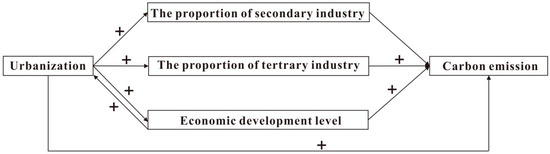
Figure 4.
The significant impact path of urbanization on carbon emissions.
In Figure 4, “+” represents a positive promotion effect, the proportion of second industry (lnC1) has no significant positive effect on carbon emissions (lnY). It can be seen that the pathway of urbanization → the proportion of second industry (the proportion of third industry, economic development level) → carbon emissions and economic development → urbanization → carbon emissions plays a significant role.
4. Conclusions and Discussions
Based on the carbon emissions data of the Yangtze River Delta region in 2008–2015, this paper undertook the research regarding the impact path of urbanization to carbon emissions. When compared with previous studies, firstly, the results of different scales are compared and the optimal scale is selected by using the method of scale variance decomposition, which makes the study of different scales more objective. Secondly, based on spatial correlation, this paper improves the previous research methods. Finally, we consider the relationship between the research objects and study the influence path of urbanization on carbon emissions through the correlation variables, which extend the connotation of energy and environment.
4.1. Conclusions
The main results show as following:
(1) There is a positive spatial correlation of carbon emissions in the Yangtze River Delta. In some cities, there is a phenomenon of “being a neighbor” when laying out high-energy enterprises.
(2) The scale effect of urbanization on carbon emissions has not yet appeared. Urbanization has significantly affected the industrial structure of the region, and of the pathway of urbanization → the proportion of second industry (the proportion of third industry, economic development level) → carbon emissions play a significant role, but there is no mechanism for the economic development level to adversely affect the level of urbanization and thus affect carbon emissions.
(3) The increase in urbanization rate has provided more employment opportunities for the society, but the promotion of social employment level has not promoted the development of regional economic development. From the urbanization level to the employment level, to the economic development level, to the carbon emission linkage path, is not significant. However, there is no mechanism for the economic development level to adversely affect the level of urbanization and thus affect carbon emissions.
4.2. Discussions
4.2.1. Discussion on the Results of Scale Variance Decomposition
This section estimates the carbon emissions of provinces, cities, and counties in the Yangtze River Delta region and the present situation is briefly analyzed. The results of the scale analysis of variance show that, from 2008 to 2015, at the county level, carbon emissions carry the largest amount of information, and their contribution rate is higher than those of the provincial and municipal scales, accounting for over 50% of the total information, on average. The contributions of the provincial and municipal scales have remained at a level of 23%. This may be because the imbalance between the regional developments has led to huge differences in carbon emissions. From the perspective of regional dimensions, Jiangsu province has the highest carbon emission level and the differences between Shanghai and Zhejiang are relatively small. At the municipal scale, the regional differences in carbon emissions within the Yangtze River Delta urban agglomeration are very large, the carbon emissions in the central region are high, and the carbon emissions in the north and south are relatively low. Therefore, it is especially important to further optimize the urban industrial structure and change the traditional extensive mode of production.
4.2.2. Discussion on the Results of Spatial Analysis of Carbon Emissions
This section analyzes the spatial correlation of carbon emissions and the results show that the carbon emissions in the Yangtze River Delta region are negatively correlated with the adjacent spatial weight matrix; but at the 10% significance level, this negative spatial correlation is insignificant. This negative spatial correlation may be due to the blurring of administrative boundaries in different urban areas on the county scale. Regarding economic distance and space weight, at the 5% significance level, there is a positive spatial correlation between carbon emissions in areas of similar economic development; this shows that carbon emissions from regions with similar levels of economic development are similar. The reason is that areas with similar levels of economic development learn and influence each other in the process of urbanization, industrial planning, and economic development planning.
4.2.3. Discussion on the Results of the Significant Impact Path of Urbanization on Carbon Emissions
This section analyzes the significant impact path of urbanization on carbon emissions, with the results illustrating that there are three action paths: urbanization → the proportion of second industry (the proportion of third industry, economic development level) → carbon emissions and economic development → urbanization → carbon emissions. This may be because urbanization has promoted large scale infrastructure construction and housing construction in the region, which results in a large amount of energy consumption. At the same time, the level of economic development is also an important factor to promote the urbanization process of the Yangtze River Delta urban agglomeration. Therefore, in order to reduce carbon emissions and achieve low-carbon development of the regional economy, the industrial structure should be optimized in the process of urbanization promotion. On the other hand, we should increase the level of investment in environmental management of the secondary industry, such as urging high-energy-consuming enterprises to purchase energy saving and environmental protection devices.
4.3. Policy Implications
Based on our research results, the main policy implications of our proposals are as follows:
(1) Developing a low-carbon industry. All of the regions should have a holistic view on reducing carbon emissions and achieving regional low-carbon development, and strengthening cross-regional cooperation. Some cities should play a “demonstration effect” of carbon emission reduction, achieve “coordinated development” of low-carbon economy among regions, and eliminate the emergence of the phenomenon of “being a neighbour”. Low-carbon industrial clusters, including thermal power emission reduction, industrial energy saving and emission reduction, energy-saving buildings, resource recycling, environmental protection equipment, energy-saving materials, and other low-carbon industrial clusters should be vigorously developed. Vigorously promote scientific and technological progress, enhance enterprise technology and equipment capabilities, and adopt low-carbon technologies to improve energy efficiency. Develop and utilize new clean energy sources, such as solar, wind, and nuclear energy, and gradually change the traditional energy structure.
(2) Carbon emissions can be effectively curbed by optimizing urban industrial structure and upgrading industrial structure. It is necessary to take urbanization as an opportunity for industrial adjustment, guide the national economy to take the secondary and tertiary industries as the leading role, appropriately restrict the development of high-energy-consuming industries, and vigorously develop low-carbon service industries.
(3) The government should properly control the speed and scale of urbanization and control the urbanization as an opportunity for low-carbon development. The rapid growth of carbon emissions has improved the transportation network within and between cities, strengthened the communication and communication between cities, and clearly defined the functions of each city from the perspective of the city. The role of the central city in the radiation of surrounding towns and villages should be emphasized, an improvement of the overall urbanization level in the region should be promoted, and the development of a low-carbon economy within the region should be promoted.
Author Contributions
F.W. and J.L. conceived the idea of this paper; J.L. provided financial support; G.W. and M.G. performed the model; M.G. analyzed the data; Y.Q. finished the first draft; G.W., L.J., W.F. assisted in modifying the paper and translating papers. All the authors read and confirmed the final manuscript.
Acknowledgments
This work was supported by the National Natural Science Foundation of China (Grant No. 71673270; No. 71403268), China Scholarship Council Project (Grant No. 201806425016).
Conflicts of Interest
The authors declare no conflict of interest.
References
- Dong, F.; Yu, B.; Hadachin, T.; Dai, Y.; Wang, Y. Drivers of carbon emission intensity change in China. Resour. Conserv. Recycl. 2018, 129, 187–201. [Google Scholar] [CrossRef]
- Johnson, H.E.; Sushinsky, J.R.; Holland, A.; Bergman, E.J.; Balzer, T. Increases in Residential and Energy Development are Associated with Reductions in Recruitment for a Large Ungulate. Glob. Chang. Biol. 2017, 2, 578–591. [Google Scholar] [CrossRef] [PubMed]
- Zhang, Y.J.; Yi, W.C.; Li, B.W. The Impact of Urbanization on Carbon Emission: Empirical Evidence in Beijing. Energy Procedia 2015, 75, 2963–2968. [Google Scholar] [CrossRef]
- Ren, L.; Wang, W.; Wang, J.; Liu, R. Analysis of Energy Consumption and Carbon Emission during the Urbanization of Shandong Province, China. J. Clean. Prod. 2015, 103, 534–541. [Google Scholar] [CrossRef]
- Sheng, P.; Guo, X. The Long-Run and Short-Run Impacts of Urbanization on Carbon Dioxide Emissions. Econ. Model. 2016, 53, 208–215. [Google Scholar] [CrossRef]
- Li, K.; Lin, B. Impacts of Urbanization and Industrialization on Energy Consumption/Emissions: Does the Level of Development Matter? Renew. Sustain. Energy Rev. 2015, 52, 1107–1122. [Google Scholar] [CrossRef]
- Dong, X.; Yuan, G. China’s Greenhouse Gas Emissions Dynamic Effects in the Process of Its Urbanization: A Perspective from Shocks Decomposition under Long-Term Constraints. Energy Procedia 2011, 5, 1660–1665. [Google Scholar]
- Li, C.; Kuang, Y.; Huang, N.; Zhang, C. The Long-Term Relationship between Population Growth and Vegetation Cover: An Empirical Analysis Based on the Panel Data of 21 Cities in Guangdong Province, China. Int. J. Environ. Res. Public Health 2013, 2, 660–677. [Google Scholar] [CrossRef] [PubMed]
- Cole, M.; Neumayer, E. Examining the Impact of Demographic Factors on Air Pollution. Popul. Environ. 2004, 1, 5–21. [Google Scholar] [CrossRef]
- Yang, Y.; Zhao, T.; Wang, Y.; Shi, Z. Research on Impacts of Population-Related Factors on Carbon Emissions in Beijing from 1984 to 2012. Environ. Impact Assess. Rev. 2015, 55, 45–53. [Google Scholar] [CrossRef]
- Wang, H.; Wang, Y.; Wang, H.; Liu, M.; Zhang, Y. Mitigating Greenhouse Gas Emissions from China’s Cities: Case Study of Suzhou. Energy Policy 2014, 68, 482–489. [Google Scholar] [CrossRef]
- York, R. Demographic Trends and Energy Consumption in European Union Nations, 1960–2025. Soc. Sci. Res. 2007, 3, 855–872. [Google Scholar] [CrossRef]
- Liddle, B.; Lung, S. Age-Structure, Urbanization, and Climate Change in Developed Countries: Revisiting Stirpat for Disaggregated Population and Consumption-Related Environmental Impacts. Popul. Environ. 2010, 5, 317–343. [Google Scholar] [CrossRef]
- Wang, Y.; Li, L.; Kubota, J.; Han, R.; Zhu, X. Does Urbanization Lead to More Carbon Emission? Evidence from a Panel of Brics Countries. Appl. Energy 2016, 168, 375–380. [Google Scholar] [CrossRef]
- York, R.; Rosa, E.A.; Dietz, T. A Rift in Modernity? Assessing the Anthropogenic Sources of Global Climate Change with the Stirpat Model. Int. J. Sociol. Soc. Policy 2003, 10, 31–51. [Google Scholar] [CrossRef]
- Sharma, S.S. Determinants of Carbon Dioxide Emissions: Empirical Evidence from 69 Countries. Appl. Energy 2011, 1, 376–382. [Google Scholar] [CrossRef]
- Xu, H.; Zhang, W. The Causal Relationship between Carbon Emissions and Land Urbanization Quality: A Panel Data Analysis for Chinese Provinces. J. Clean. Prod. 2016, 137, 241–248. [Google Scholar] [CrossRef]
- Ali, H.S.; Abdul-Rahim, A.S.; Ribadu, M.B. Urbanization and Carbon Dioxide Emissions in Singapore: Evidence from the Ardl Approach. Environ. Sci. Pollut. Res. Int. 2017, 2, 1967–1974. [Google Scholar] [CrossRef]
- Asumadu-Sarkodie, S.; Owusu, P.A. A Multivariate Analysis of Carbon Dioxide Emissions, Electricity Consumption, Economic Growth, Financial Development, Industrialization, and Urbanization in Senegal. Energy Sources Part Econ. Plan. Policy 2017, 1, 77–84. [Google Scholar] [CrossRef]
- Wang, S.; Fang, C.; Guan, X.; Pang, B.; Ma, H. Urbanisation, Energy Consumption, and Carbon Dioxide Emissions in China: A Panel Data Analysis of China’s Provinces. Appl. Energy 2014, 136, 738–749. [Google Scholar] [CrossRef]
- Wang, Y.; Chen, L.; Kubota, J. The Relationship Between Urbanization, Energy Use and Carbon Emissions: Evidence from a Panel of Association of Southeast Asian Nations (Asean) Countries. J. Clean. Prod. 2016, 112, 1368–1374. [Google Scholar] [CrossRef]
- Ouyang, X.; Lin, B. Carbon Dioxide Emissions during Urbanization: A Comparative Study Between China and Japan. J. Clean. Prod. 2017, 143, 356–368. [Google Scholar] [CrossRef]
- Zhang, Z.; Zhao, Y.; Su, B.; Zhang, Y. Embodied Carbon in China’s Foreign Trade: An Online Sci-E and Ssci Based Literature Review. Renew. Sustain. Energy Rev. 2017, 1, 492–510. [Google Scholar] [CrossRef]
- Pacheco-Torres, R.; Roldan, J.; Gago, E.J.; Ordonez, J. Assessing the Relationship between Urban Planning Options and Carbon Emissions at the Use Stage of New Urbanized Areas: A Case Study in Warm Climate Location. Energy Build. 2017, 136, 73–85. [Google Scholar] [CrossRef]
- Wang, S.; Fang, C.; Ma, H.T. Spatial Differences and Multi-Mechanism of Carbon Footprint Based on Gwr Model in Provincial China. J. Geogr. Sci. 2014, 4, 612–630. [Google Scholar] [CrossRef]
- Xiong, C.; Yang, D.; Huo, J. Spatial-Temporal Characteristics and Lmdi-Based Impact Factor Decomposition of Agricultural Carbon Emissions in Hotan Prefecture, China. Sustainability 2016, 8, 262. [Google Scholar] [CrossRef]
- Videras, J. Exploring Spatial Patterns of Carbon Emissions in the USA: A Geographically Weighted Regression Approach. Popul. Environ. 2014, 2, 137–154. [Google Scholar] [CrossRef]
- Wang, F.; Gao, M.; Liu, J.; Fan, W. The Spatial Network Structure of China’s Regional Carbon Emissions and Its Network Effect. Energies 2018, 11, 2706. [Google Scholar] [CrossRef]
- Pan, H.; Deal, B.; Chen, Y. A Reassessment of urban structure and land-use patterns: Distance to CBD or network-based?—Evidence from Chicago. Region. Sci. Urban Econ. 2018, 70, 215–228. [Google Scholar] [CrossRef]
- Seto, K.C.; Shepherd, J.M. Global urban land-use trends and climate impacts. Curr. Opin. Environ. Sustain. 2009, 1, 89–95. [Google Scholar] [CrossRef]
- Hu, Y.; Jia, G.; Pohl, C. Improved monitoring of urbanization processes in China for regional climate impact assessment. Environ. Earth Sci. 2015, 12, 8387–8404. [Google Scholar] [CrossRef]
- Cushman, S.A.; Mcgarigal, K. Hierarchical, Multi-scale decomposition of species-environment relationships. Landsc. Ecol. 2002, 7, 637–646. [Google Scholar] [CrossRef]
- Cai, B.; Yu, R. Comparison on Spatial Scale Analysis Methods in Landscape Ecology. Acta Ecol. Sin. 2008, 5, 2279–2287. [Google Scholar]
- José, M.; María, L. Driving forces of Spain’s CO2 emissions: A LMDI decomposition approach. Renew. Sustain. Energy Rev. 2015, 48, 749–759. [Google Scholar]
- Jung, S.; Kyoungjin, A.N. Regional energy-related carbon emission characteristics and potential mitigation in eco-industrial parks in South Korea: Logarithmic mean Divisia index analysis based on the Kaya identity. Energy 2012, 1, 231–241. [Google Scholar] [CrossRef]
- Budzianowski, W.M. Modelling of CO2 content in the atmosphere until 2300: Influence of energy intensity of gross domestic product and carbon intensity of energy. Inter. J. Glob. Warm. 2013, 1, 1–17. [Google Scholar] [CrossRef]
- Hu, J.; Jiang, X. Study on the Influence of Urbanization on Carbon Emissions from the Perspective of Urban Agglomeration. J. China Univ. Geosci. 2015, 6, 11–21. [Google Scholar]
- Chuntao, W.U. The Impact of Urbanization on Agricultural Carbon Emissions in China—An Empirical Study Based on Provincial Data. Econ. Surv. 2015, 1, 12–18. [Google Scholar]
- Wang, G. Urbanization: Focus of the Transformation of China’s Economic Development Model. Econ. Res. 2010, 12, 43–59. [Google Scholar]
- Tao, A.; Yang, S.; Li, Y. The Impact of Urbanization Quality on the Spatial Effects of Carbon Emissions: A Case Study of 16 Cities in the Yangtze River Delta Region. Urban Probl. 2016, 12, 11–18. [Google Scholar]
- Huo, B. Research on the Influencing Factors of the Differences of Urbanization Development in China: Based on the Empirical Analysis of Provincial Panel Data from 1992 to 2015. Inq. Econ. Issues 2017, 4, 76–82. [Google Scholar]
- Yang, G.; Wu, Q.; Tu, Y. Researchs of China’s Regional Carbon Emission Spatial Correlation and Its Determinants: Based on the Method of Social Network Analysis. J. Bus. Econ. 2016, 4, 56–68. [Google Scholar]


© 2019 by the authors. Licensee MDPI, Basel, Switzerland. This article is an open access article distributed under the terms and conditions of the Creative Commons Attribution (CC BY) license (http://creativecommons.org/licenses/by/4.0/).