Figure 1.
The paving of the Fast Kurtogram.
Figure 1.
The paving of the Fast Kurtogram.
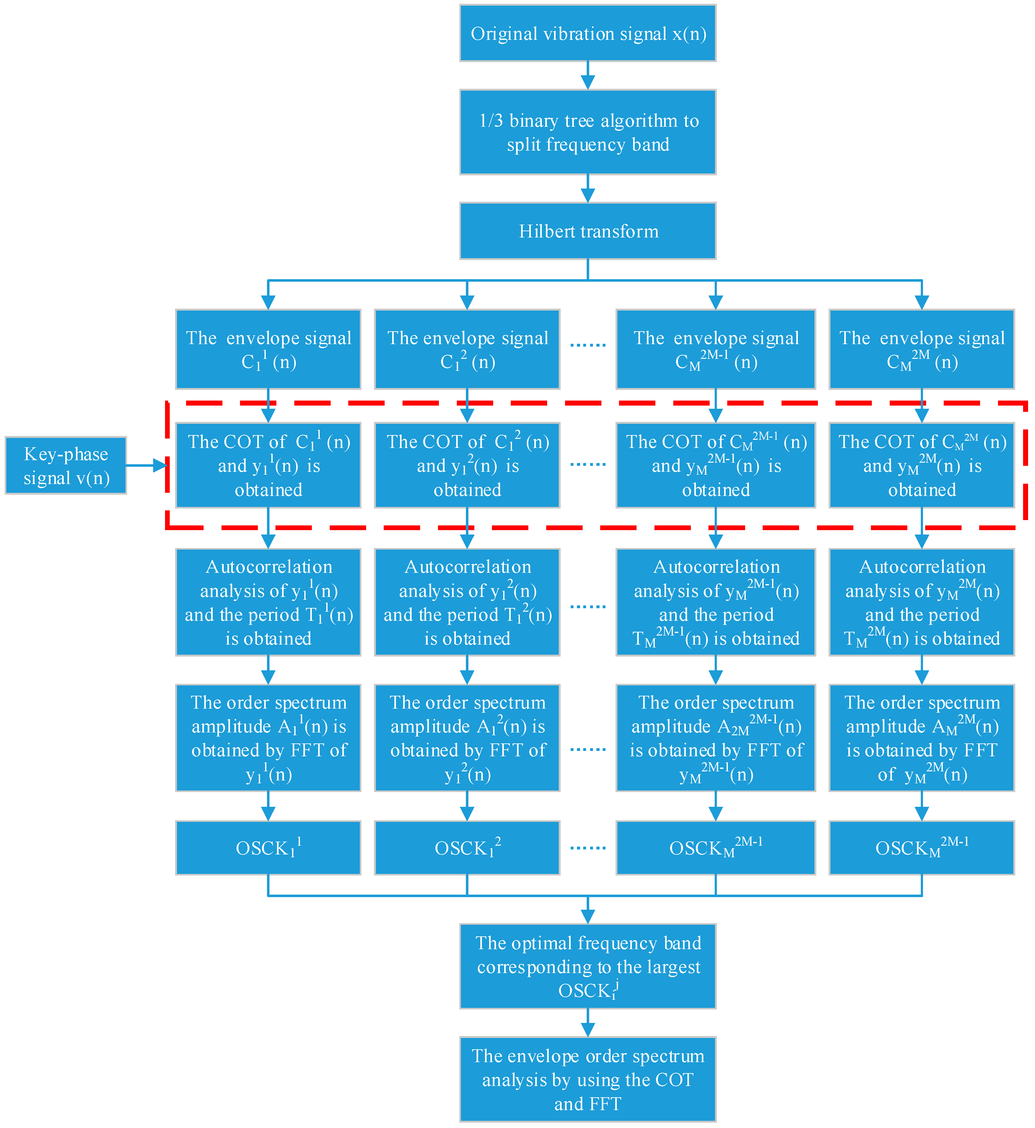
Figure 2.
The flowchart of proposed method.
Figure 2.
The flowchart of proposed method.
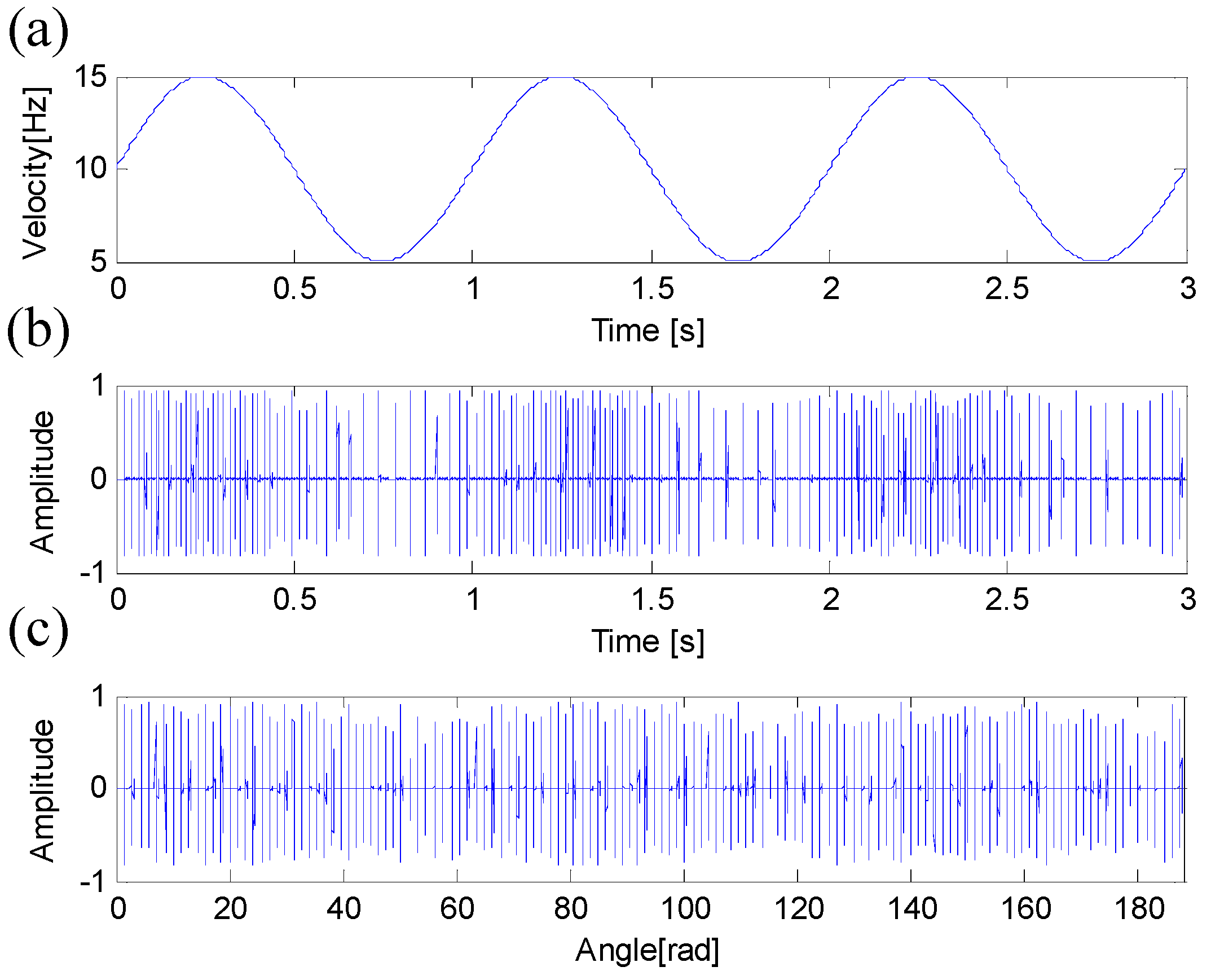
Figure 3.
Simple simulation: (a) the shaft rotational frequency, (b) the impulse signal in the time domain and (c) the resampling signal in the angle domain.
Figure 3.
Simple simulation: (a) the shaft rotational frequency, (b) the impulse signal in the time domain and (c) the resampling signal in the angle domain.
Figure 4.
STFTs of the simulation: (a) STFT of the time-domain signal and (b) STFT of the angular-domain signal.
Figure 4.
STFTs of the simulation: (a) STFT of the time-domain signal and (b) STFT of the angular-domain signal.
Figure 5.
Envelopes of the filtered signals: (a) envelope of the time-domain filtered signal and (b) envelope of the angular-domain filtered signal.
Figure 5.
Envelopes of the filtered signals: (a) envelope of the time-domain filtered signal and (b) envelope of the angular-domain filtered signal.
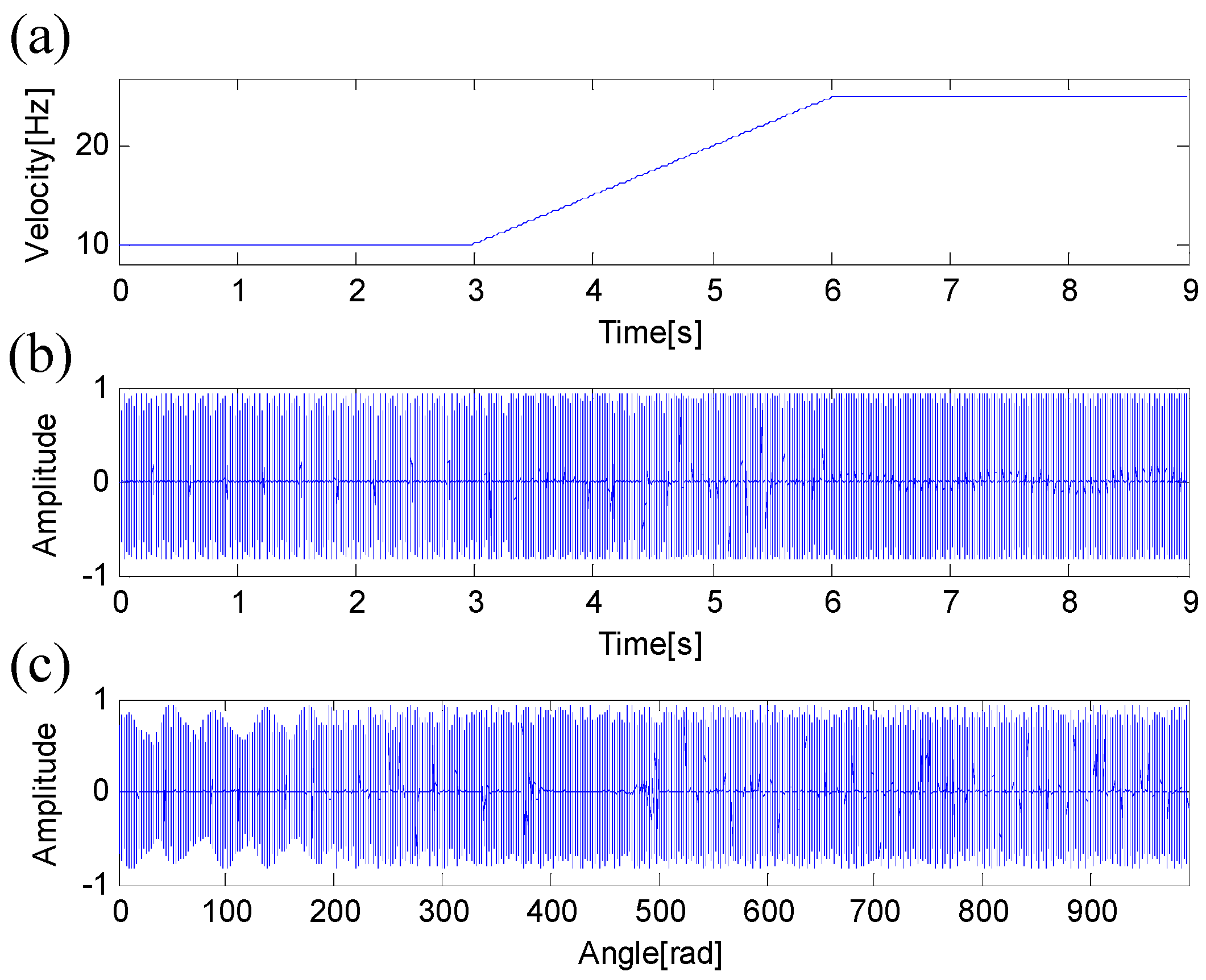
Figure 6.
Simple simulation: (a) the shaft rotational frequency, (b) the impulse signal in the time domain and (c) the resampling signal in angle domain.
Figure 6.
Simple simulation: (a) the shaft rotational frequency, (b) the impulse signal in the time domain and (c) the resampling signal in angle domain.
Figure 7.
(a) The shaft rotational frequency, (b) the normalized kurtosis of different indexes.
Figure 7.
(a) The shaft rotational frequency, (b) the normalized kurtosis of different indexes.
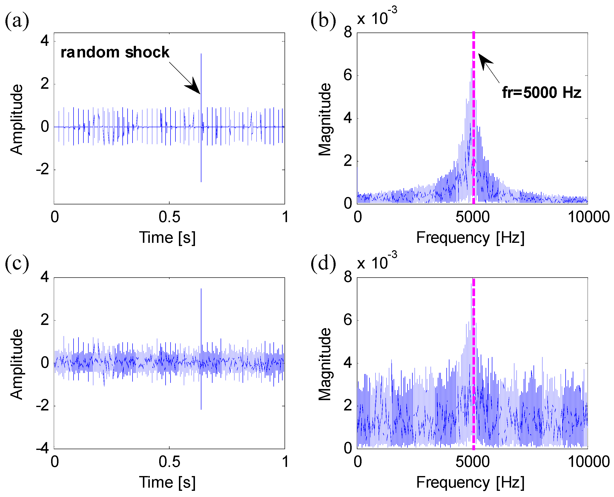
Figure 8.
Simple simulation: (a) the simulated signal, (b) the frequency spectra of (a), (c) the noise-added signal with SNR = −5 dB and (d) the frequency spectra of (c).
Figure 8.
Simple simulation: (a) the simulated signal, (b) the frequency spectra of (a), (c) the noise-added signal with SNR = −5 dB and (d) the frequency spectra of (c).
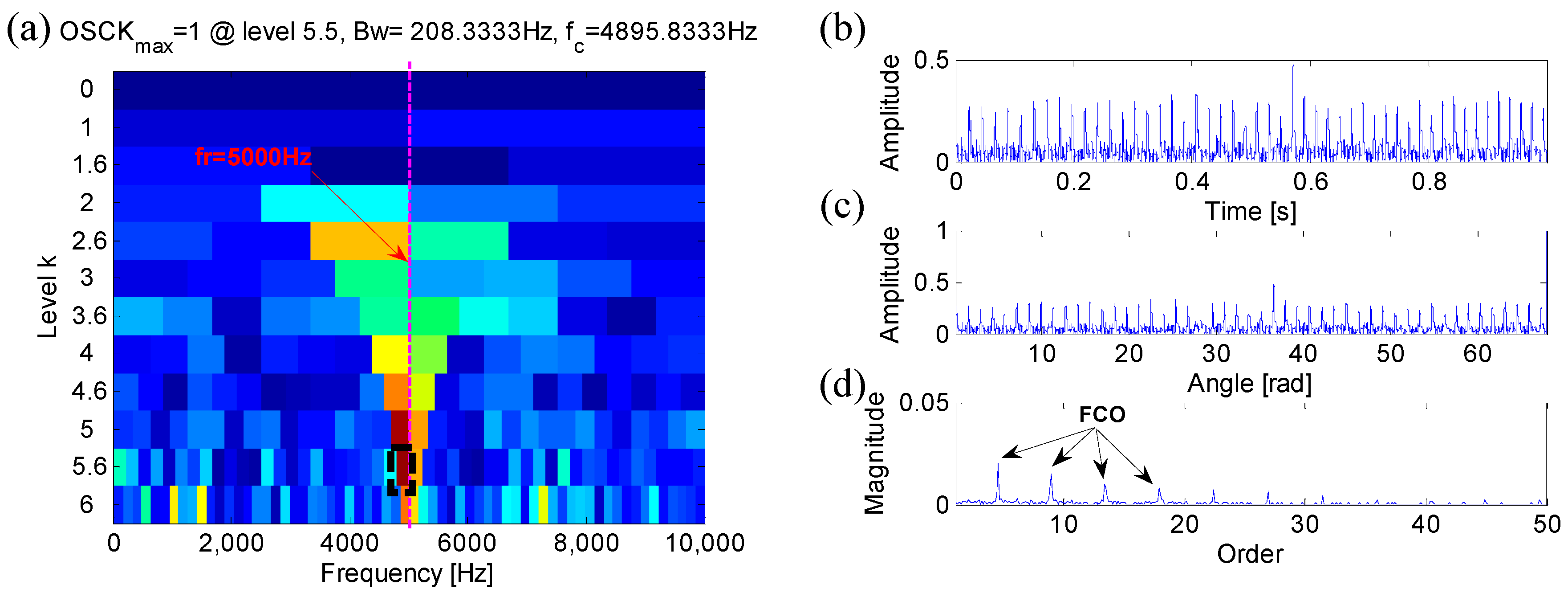
Figure 9.
The results obtained by the FOSCK for processing the mixed signal with same resonant frequency: (a) FOSCK, (b) the envelope of the band-pass filtered signal, (c) the resampling envelope signal of (b,d) the envelope order spectrum of (c).
Figure 9.
The results obtained by the FOSCK for processing the mixed signal with same resonant frequency: (a) FOSCK, (b) the envelope of the band-pass filtered signal, (c) the resampling envelope signal of (b,d) the envelope order spectrum of (c).
Figure 10.
Simple simulation: (a) the simulated signal, (b) the frequency spectra of (a), (c) the noise-added signal with SNR= −5 dB and (d) the frequency spectra of (c).
Figure 10.
Simple simulation: (a) the simulated signal, (b) the frequency spectra of (a), (c) the noise-added signal with SNR= −5 dB and (d) the frequency spectra of (c).
Figure 11.
The results obtained by the FOSCK for processing the mixed signal with different resonant frequencies: (a) FOSCK, (b) the envelope of the band-pass filtered signal, (c) the resampling envelope signal of (b,d) the envelope order spectrum of (c).
Figure 11.
The results obtained by the FOSCK for processing the mixed signal with different resonant frequencies: (a) FOSCK, (b) the envelope of the band-pass filtered signal, (c) the resampling envelope signal of (b,d) the envelope order spectrum of (c).
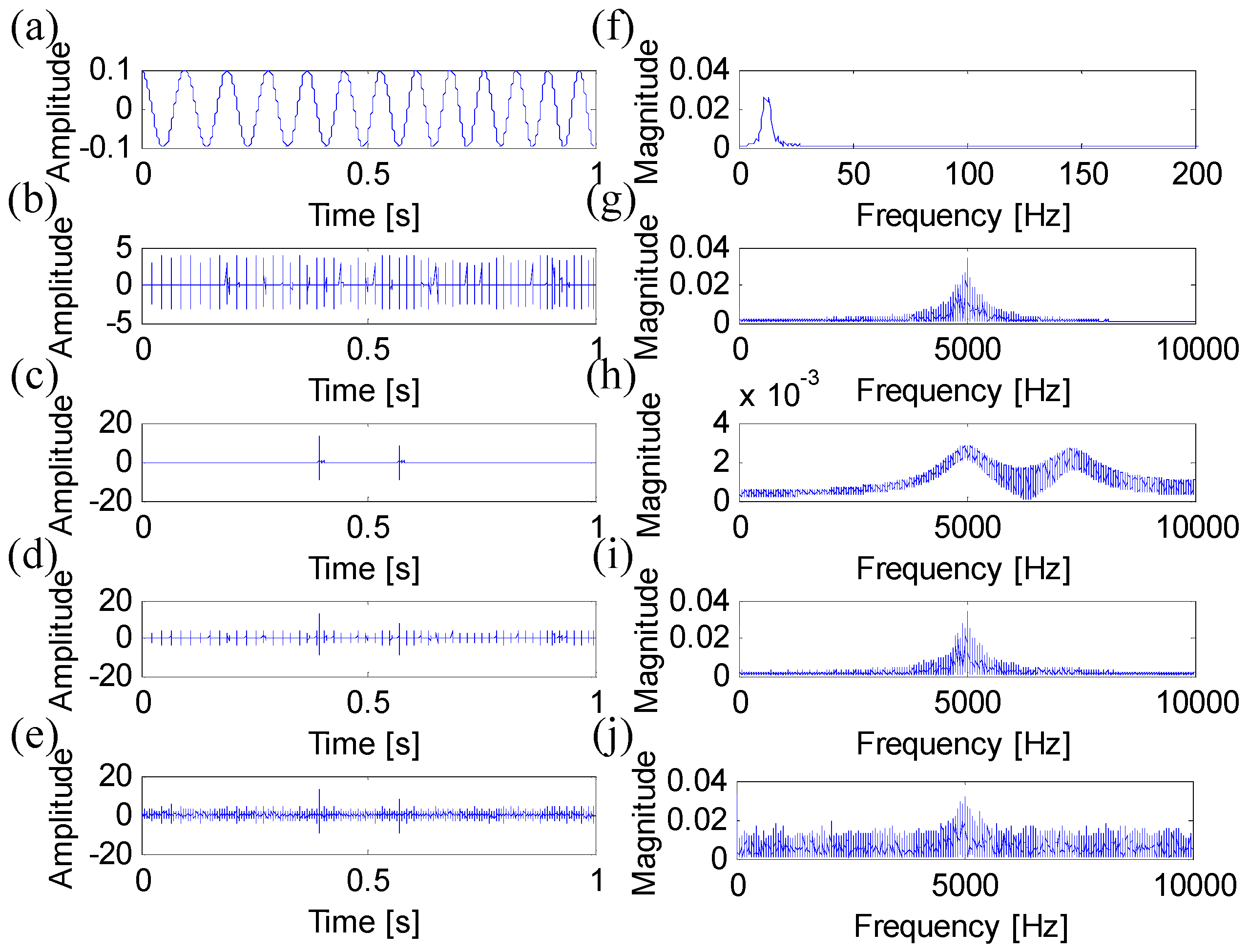
Figure 12.
Simulated signals: (a) a deterministic component signal, (b) the fault impulse signal, (c) the random shocks, (d) the synthetic signal without noise added, (e) the synthetic signal with noise-added and SNR = −5 and (f–j) the frequency spectra of the different components.
Figure 12.
Simulated signals: (a) a deterministic component signal, (b) the fault impulse signal, (c) the random shocks, (d) the synthetic signal without noise added, (e) the synthetic signal with noise-added and SNR = −5 and (f–j) the frequency spectra of the different components.
Figure 13.
The results obtained by the FK for processing the mixed signal: (a) FK, (b) the envelope of the band-pass filtered signal, (c) the resampling envelope signal of (b,d) the envelope order spectrum of (c).
Figure 13.
The results obtained by the FK for processing the mixed signal: (a) FK, (b) the envelope of the band-pass filtered signal, (c) the resampling envelope signal of (b,d) the envelope order spectrum of (c).
Figure 14.
The results obtained by the WPTK for processing the mixed signal: (a) WPTK, (b) the envelope of the band-pass filtered signal, (c) the envelope of the resampling of (b,d) the envelope order spectrum of (c).
Figure 14.
The results obtained by the WPTK for processing the mixed signal: (a) WPTK, (b) the envelope of the band-pass filtered signal, (c) the envelope of the resampling of (b,d) the envelope order spectrum of (c).
Figure 15.
The results obtained by the Protrugram for processing the mixed signal: (a) Protrugram, (b) the envelope of the band-pass filtered signal, (c) the envelope of the resampling of (b,d) the envelope order spectrum of (c).
Figure 15.
The results obtained by the Protrugram for processing the mixed signal: (a) Protrugram, (b) the envelope of the band-pass filtered signal, (c) the envelope of the resampling of (b,d) the envelope order spectrum of (c).
Figure 16.
The results obtained by the FOSCK for processing the mixed signal: (a) FOSCK, (b) the envelope of the band-pass filtered signal, (c) the envelope of the resampling of (b,d) the envelope order spectrum of (c).
Figure 16.
The results obtained by the FOSCK for processing the mixed signal: (a) FOSCK, (b) the envelope of the band-pass filtered signal, (c) the envelope of the resampling of (b,d) the envelope order spectrum of (c).
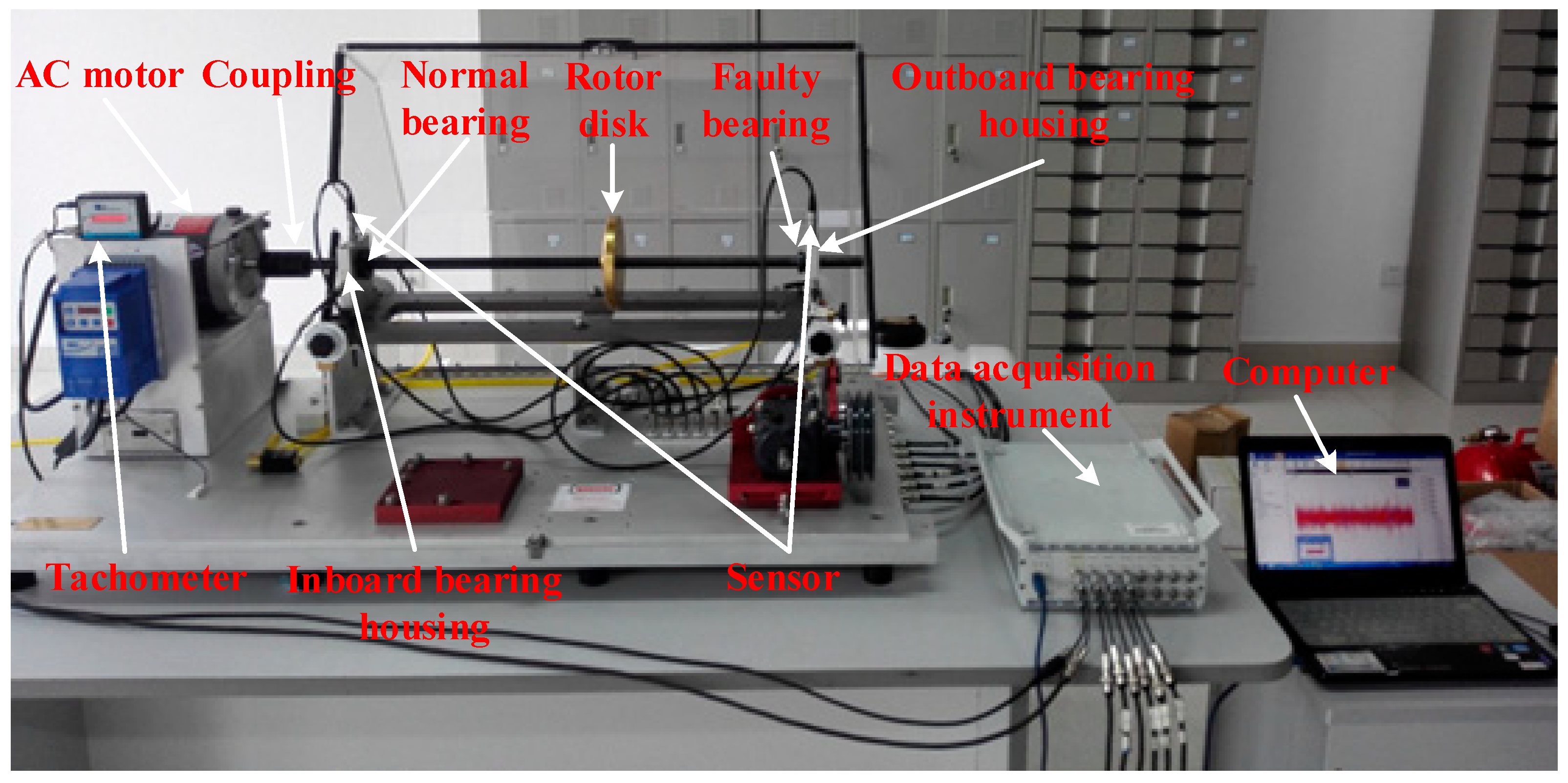
Figure 17.
The test bench for bearing fault detection.
Figure 17.
The test bench for bearing fault detection.
Figure 18.
The signal measured from a normal bearing: (a) time-domain signal, (b) the shaft rotational frequency from 20 Hz to 25 Hz, (c) the frequency spectrum of (a,d) TFR by using STFT.
Figure 18.
The signal measured from a normal bearing: (a) time-domain signal, (b) the shaft rotational frequency from 20 Hz to 25 Hz, (c) the frequency spectrum of (a,d) TFR by using STFT.
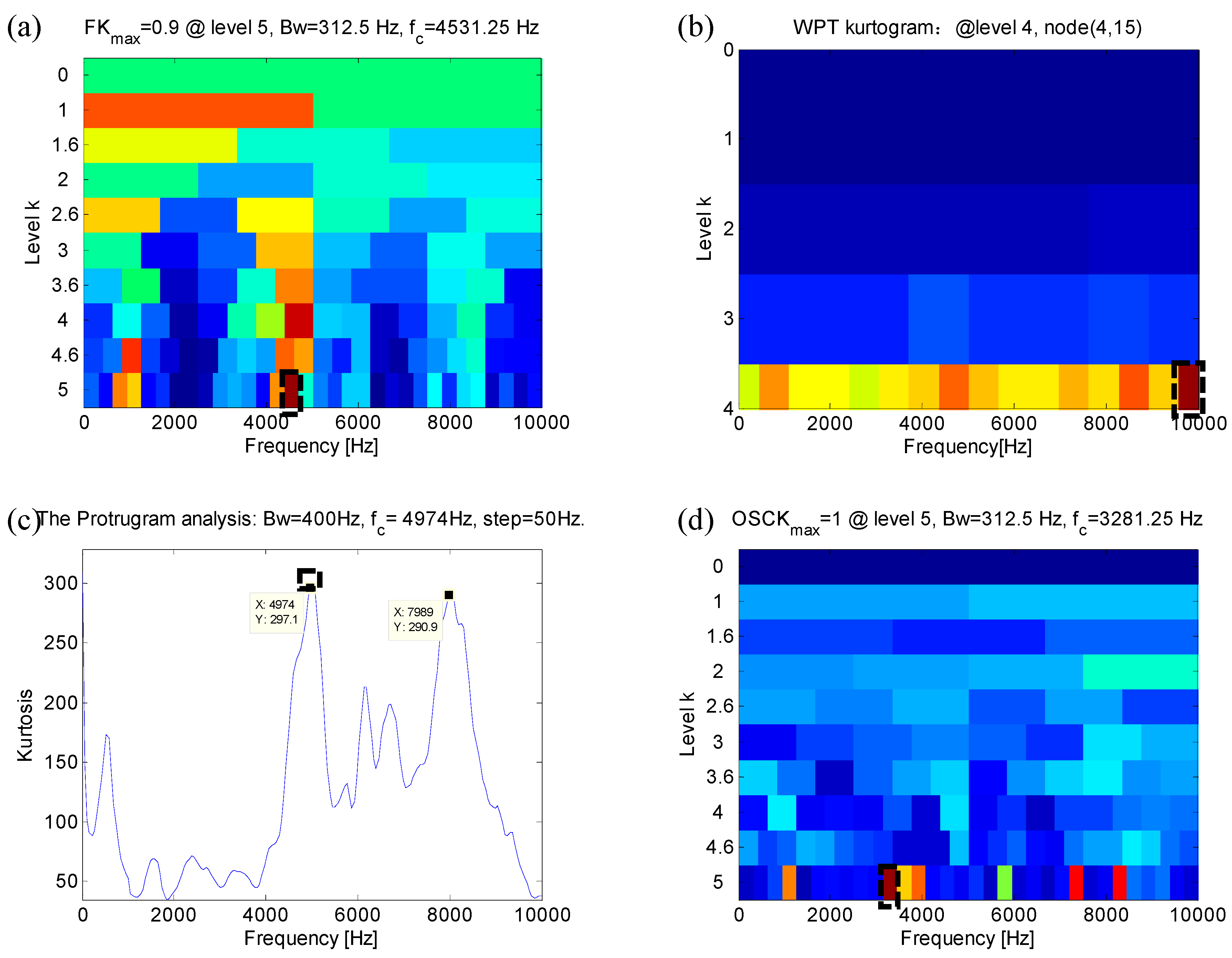
Figure 19.
The optimal frequency band obtained by different methods: (a) FK, (b) WPTK, (c) Protrugram and (d) FOSCK.
Figure 19.
The optimal frequency band obtained by different methods: (a) FK, (b) WPTK, (c) Protrugram and (d) FOSCK.
Figure 20.
The envelope order spectra of the signal obtained by different methods: (a) FK, (b) WPTK, (c) Protrugram and (d) FOSCK.
Figure 20.
The envelope order spectra of the signal obtained by different methods: (a) FK, (b) WPTK, (c) Protrugram and (d) FOSCK.
Figure 21.
The signal measured from an outer race fault bearing: (a) time-domain signal, (b) the shaft rotational frequency from 20 Hz to 25 Hz, (c) the frequency spectrum of (a,d) TFR by using STFT.
Figure 21.
The signal measured from an outer race fault bearing: (a) time-domain signal, (b) the shaft rotational frequency from 20 Hz to 25 Hz, (c) the frequency spectrum of (a,d) TFR by using STFT.
Figure 22.
The optimal frequency band obtained by different methods: (a) FK, (b) WPTK, (c) Protrugram and (d) FOSCK.
Figure 22.
The optimal frequency band obtained by different methods: (a) FK, (b) WPTK, (c) Protrugram and (d) FOSCK.
Figure 23.
The envelope order spectra of the signal obtained by different methods: (a) FK, (b) WPTK, (c) Protrugram and (d) FOSCK.
Figure 23.
The envelope order spectra of the signal obtained by different methods: (a) FK, (b) WPTK, (c) Protrugram and (d) FOSCK.
Figure 24.
The signal measured from an outer race fault bearing: (a) time-domain signal, (b) the shaft rotational frequency from 20 Hz to 25 Hz, (c) the frequency spectrum of (a,d) TFR by using STFT.
Figure 24.
The signal measured from an outer race fault bearing: (a) time-domain signal, (b) the shaft rotational frequency from 20 Hz to 25 Hz, (c) the frequency spectrum of (a,d) TFR by using STFT.
Figure 25.
The optimal frequency band obtained by different methods: (a) FK, (b) WPTK, (c) Protrugram and (d) FOSCK.
Figure 25.
The optimal frequency band obtained by different methods: (a) FK, (b) WPTK, (c) Protrugram and (d) FOSCK.
Figure 26.
The envelope order spectra of the signal obtained by different methods: (a) FK, (b) WPTK, (c) Protrugram and (d) FOSCK.
Figure 26.
The envelope order spectra of the signal obtained by different methods: (a) FK, (b) WPTK, (c) Protrugram and (d) FOSCK.
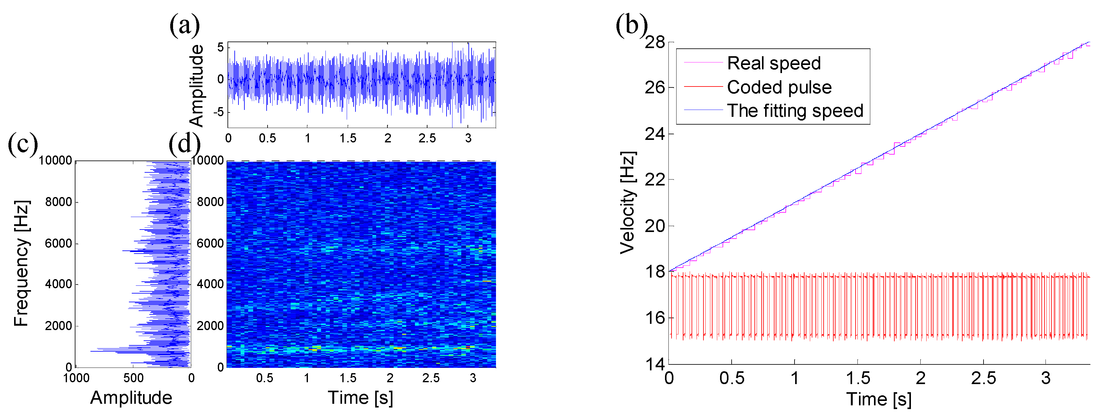
Figure 27.
The signal measured from an outer race fault bearing: (a) time-domain signal, (b) the shaft rotational frequency from 18 Hz to 28 Hz, (c) the frequency spectrum of (a,d) TFR by using STFT.
Figure 27.
The signal measured from an outer race fault bearing: (a) time-domain signal, (b) the shaft rotational frequency from 18 Hz to 28 Hz, (c) the frequency spectrum of (a,d) TFR by using STFT.
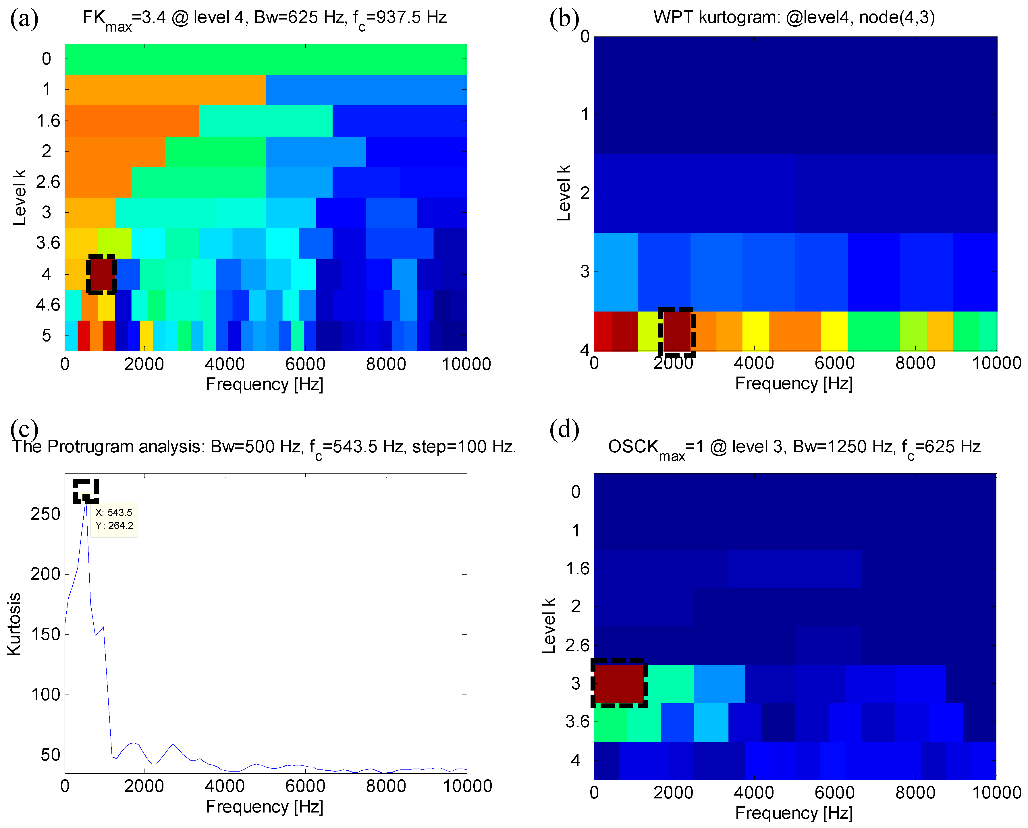
Figure 28.
The optimal frequency band obtained by different methods: (a) FK, (b) WPTK, (c) Protrugram and (d) FOSCK.
Figure 28.
The optimal frequency band obtained by different methods: (a) FK, (b) WPTK, (c) Protrugram and (d) FOSCK.
Figure 29.
The envelope order spectra of the signal obtained by different methods: (a) FK, (b) WPTK, (c) Protrugram and (d) FOSCK.
Figure 29.
The envelope order spectra of the signal obtained by different methods: (a) FK, (b) WPTK, (c) Protrugram and (d) FOSCK.
Figure 30.
The signal measured from an inner race fault bearing: (a) time-domain signal, (b) the shaft rotational frequency from 20 Hz to 25 Hz, (c) the frequency spectrum of (a,d) TFR by using STFT.
Figure 30.
The signal measured from an inner race fault bearing: (a) time-domain signal, (b) the shaft rotational frequency from 20 Hz to 25 Hz, (c) the frequency spectrum of (a,d) TFR by using STFT.
Figure 31.
The optimal frequency band obtained by different methods: (a) FK, (b) WPTK, (c) Protrugram and (d) FOSCK.
Figure 31.
The optimal frequency band obtained by different methods: (a) FK, (b) WPTK, (c) Protrugram and (d) FOSCK.
Figure 32.
The envelope order spectra of the signal obtained by different methods: (a) FK, (b) WPTK, (c) Protrugram and (d) FOSCK.
Figure 32.
The envelope order spectra of the signal obtained by different methods: (a) FK, (b) WPTK, (c) Protrugram and (d) FOSCK.
Figure 33.
The signal measured from an inner race fault bearing: (a) time-domain signal, (b) the shaft rotational frequency from 20 Hz to 25 Hz, (c) the frequency spectrum of (a,d) TFR by using STFT.
Figure 33.
The signal measured from an inner race fault bearing: (a) time-domain signal, (b) the shaft rotational frequency from 20 Hz to 25 Hz, (c) the frequency spectrum of (a,d) TFR by using STFT.
Figure 34.
The optimal frequency band obtained by different methods: (a) FK, (b) WPTK, (c) Protrugram and (d) FOSCK.
Figure 34.
The optimal frequency band obtained by different methods: (a) FK, (b) WPTK, (c) Protrugram and (d) FOSCK.
Figure 35.
The envelope order spectra of the signal obtained by different methods: (a) FK, (b) WPTK, (c) Protrugram and (d) FOSCK.
Figure 35.
The envelope order spectra of the signal obtained by different methods: (a) FK, (b) WPTK, (c) Protrugram and (d) FOSCK.
Figure 36.
The signal measured from an inner race fault bearing: (a) time-domain signal, (b) the shaft rotational frequency from 18 Hz to 28 Hz, (c) the frequency spectrum of (a,d) TFR by using STFT.
Figure 36.
The signal measured from an inner race fault bearing: (a) time-domain signal, (b) the shaft rotational frequency from 18 Hz to 28 Hz, (c) the frequency spectrum of (a,d) TFR by using STFT.
Figure 37.
The optimal frequency band obtained by different methods: (a) FK, (b) WPTK, (c) Protrugram and (d) FOSCK.
Figure 37.
The optimal frequency band obtained by different methods: (a) FK, (b) WPTK, (c) Protrugram and (d) FOSCK.
Figure 38.
The envelope order spectra of the signal obtained by different methods: (a) FK, (b) WPTK, (c) Protrugram and (d) FOSCK.
Figure 38.
The envelope order spectra of the signal obtained by different methods: (a) FK, (b) WPTK, (c) Protrugram and (d) FOSCK.
Table 1.
Parameters of the simulation model.
Table 1.
Parameters of the simulation model.
| N (s) | Bn | φm | f (Hz) | fo | fs (kHz) | fr (kHz) | β (kHz) | τn |
|---|
| 3 | 1 | 0 | 5–15 | 4.5 | 20 | 5 | 1.2 | 0.01 |
Table 2.
Parameters of the simulation model.
Table 2.
Parameters of the simulation model.
| | N (s) | Bn | φm | f (Hz) | fo | fs (kHz) | fr1 (kHz) | fr2 (kHz) | β1 (kHz) | β2 (kHz) | τn | SNR (dB) |
|---|
| Case 1 | 1 | 1 | 0 | 10–12 | 4.5 | 20 | 5 | \ | 1.2 | 3 | 0.01 | −5 |
| Case 2 | 1 | 1 | 0 | 10–12 | 4.5 | 20 | 5 | 7.3 | 1.2 | 3 | 0.01 | −5 |
Table 3.
Parameters of the simulation model.
Table 3.
Parameters of the simulation model.
| N (s) | Bn | φm | f (Hz) | fo | fs (kHz) | fr1 (kHz) | fr2 (kHz) | β1 (kHz) | β2 (kHz) | τn | SNR (dB) |
|---|
| 1 | 1 | 0 | 10–15 | 4.5 | 20 | 5 | 7.3 | 1.2 | 3 | 0.01 | −5 |
Table 4.
Parameters of the bearings.
Table 4.
Parameters of the bearings.
| Fault Severity | Bearing Type | Number of Balls | Contact Angle | Pitch Diameter | Ball Diameter | BPFO | BPFI |
|---|
| 3/4” Rotor bearing | ER-12K | 8 | 0 | 1.318 in | 0.3125 in | 3.048 | 4.95 |
Table 5.
Parameters of each experiment.
Table 5.
Parameters of each experiment.
| Acceleration (Hz/s) | Experimental Study #1 | Experimental Study #2 | Experimental Study #3 |
|---|
| a | 4/3 | 3/2 | 3 |
Table 6.
Parameters of each experiment.
Table 6.
Parameters of each experiment.
| Acceleration (Hz/s) | Experimental Study #4 | Experimental Study #5 | Experimental Study #6 |
|---|
| a | 4/3 | 3/2 | 3 |
Table 7.
Bearing fault diagnosis result.
Table 7.
Bearing fault diagnosis result.
| Fault Location | Outer Race Fault | Inner Race Fault |
|---|
| Experimental Study | #1 | #2 | #3 | #4 | #5 | #6 |
|---|
| FK | Y | N | Y | N | N | N |
| WPTK | Y | N | N | N | N | N |
| Protrugram | Y | Y | N | N | N | N |
| FOSCK | Y | Y | Y | Y | Y | Y |
Table 8.
Method robustness.
Table 8.
Method robustness.
| Interference | Random Shock | Large Speed Fluctuation | Different Acceleration | Heavy Noise |
|---|
| FK | N | Y | P | N |
| WPTK | N | N | P | N |
| Protrugram | Y | N | Y | N |
| FOSCK | Y | Y | Y | Y |


