Article

JIT Production Strategy and Maintenance for Quality Deteriorating Systems

by
Héctor Rivera-Gómez
*,
Oscar Montaño-Arango
,
José Ramón Corona-Armenta
,
Jaime Garnica-González
,
Antonio Oswaldo Ortega-Reyes
and
Gustavo Erick Anaya-Fuentes
Academic Area of Engineering, Autonomous University of Hidalgo, Pachuca-Tulancingo Road km. 4.5, City of Knowledge, Mineral de la Reforma, Hidalgo 42184, Mexico
*
Author to whom correspondence should be addressed.
Appl. Sci. 2019, 9(6), 1180; https://doi.org/10.3390/app9061180
Submission received: 28 January 2019 / Revised: 28 February 2019 / Accepted: 14 March 2019 / Published: 20 March 2019
(This article belongs to the Section Mechanical Engineering)

Abstract

:

Featured Application

The model presented in this paper can be applied in production systems composed of unreliable machines subject to deterioration whose production rates can be controlled. Examples include the systems found in important industries including: Automotive, aircraft, machine tools, semiconductor, and electronics manufacturing. Therefore, given the trade-offs related with deterioration and the strong interactions between the important functions of production planning, quality, and maintenance, advanced engineering scheduling methods such as the model presented in this paper are required to keep industries profitable.

Abstract

We study the optimal production planning and major maintenance scheduling for an unreliable manufacturing system. We assume that the production unit experiences progressive deterioration that negatively influences product quality. For the production policy, we extend improve traditional threshold policies with a superior alternative, based on a just-in-time (JIT) strategy. The paper brings a new vision on the importance of implementing more effective production strategies based on JIT methods, instead of traditional threshold policies. When a failure occurs, the production unit is minimally repaired, and when the major maintenance is selected, the machine is restored to brand-new conditions. The objective of the model is to determine the simultaneous JIT production and major maintenance strategy that minimizes the total cost. Due to the stochastic features of the system, a simulation-based optimization approach is proposed, which combines the descriptive capabilities of simulation modeling with analytical models, statistical analysis, and optimization techniques. The results verify that the proposed simulation–optimization approach provides new and coherent results that highlight the strong influence of quality deterioration on the determination of the control parameters. A sensitivity analysis and a comparative study are conducted to illustrate that significant cost savings could be obtained with the proposed approach.

1. Introduction

With the current global manufacturing context, the quality of products has become a critical factor to succeed in industrial markets. Moreover, the high variability of demand leads manufacturers to devise robust production and maintenance strategies to ensure delivery reliability. However, the current context is posing serious challenges on companies to continually reduce their costs. To cope with these challenges, advanced manufacturing systems need to be operated with balanced solutions, considering simultaneously the three key functions of production logistics, product quality, and equipment maintenance. This joint problem is particularly important in manufacturing systems prone to progressive deterioration. Nevertheless, there is a limited amount of literature dedicated to this critical problem and several important issues remain unsolved.
In this section, we discussed contributions on the production–quality connection and the production–maintenance link, since they have been the base in recent years for the development of more integrated models simultaneously addressing the functions of production–quality–maintenance. Furthermore, we present some papers on the deterioration field, because progressive degradation may considerably alter the control policy. Additionally, contributions of simulation techniques are discussed, since they are attractive solution alternatives given that analytical solutions are not available for the production systems under study because of their high stochastic complexity.
The progress in technology has allowed production managers to exercise a better control and analysis of product quality and production logistics performance. For example, a number of different kinds of analytical models focusing on the production–quality relationship have been developed in recent years, such as the paper of Kim and Gershwin [1], where numerical studies were conducted for a production system with defective production. They also successfully determined several indexes such as the total production rate, the effective production rate of conforming units, and the yield. Kim and Gershwin [2] presented an approximation method for the performance analysis of manufacturing lines with defective production. They also analyzed different versions of a production line that differs in the locations of the inspection stations and in the sets of machines that each inspection station monitors. Moreover, the results of the research carried out by Colledani and Tolio [3] have taken into account the impact of the quality control action on the production flow of parts in a system. In their model, the behavior of the production system is monitored by statistical control charts. Another analytical model has been introduced by Colledani et al. [4], where they analyzed the production rate of conforming parts for manufacturing systems with progressively deteriorating machines. In their model, they incorporated preventive maintenance. As can be noted from these papers, most of the studies have focused in the determination of performance indexes. However, the present paper aims to provide decision-makers with an integrated policy which adequately manages their production, quality, and maintenance operations in response to disruptive random events such as failures, increasing defectives, and deterioration. In particular, for the production policy, we seek to extend traditional threshold policies with superior manufacturing practices in the form of just-in-time (JIT) production strategies.
There are many studies in the literature dealing with the association between production and quality control strategies. For instance, Hajji et al. [5] studied the joint production control and product specifications with decision making. They also observed that the profit under joint production–quality and product design could increase considerably compared with the case where decisions are completely dissociated. In Bouslah et al. [6], the authors dealt with the problem of joint determination of the optimal lot sizing and production control for an unreliable production system, where the quality control of lots produced was conducted using an acceptance sampling plan. Mhada et al. [7] addressed the problem of optimal joint assignment of buffer sizes and inspection station placement for an unreliable transfer line. In their model, the location of one station is fixed to inspect finished parts, while the location of the other station is chosen to optimize the total per unit time average cost. More recently, Rivera-Gómez et al. [8] presented a model for the joint production and repair activity planning for a manufacturing system which produces defectives. In their formulation, they used an intensity control model that allowed them to implement different types of repairs, such as imperfect and minimal repairs. It is evident that quality and production modeling has been demonstrated to provide considerable advantages, as seen in these papers. Nevertheless, maintenance strategies must also be considered in these models, since these three key functions are highly coupled and optimal decisions can only be reached when these functions are captured and addressed simultaneously.
The coupling of production and maintenance strategies has been the subject of several studies in recent years. For instance, Kumar-Sharma et al. [9] proposed a framework based on failure mode effect analysis and Petri nets to analyze and predict the uncertain behavior of an industrial system. The authors aim to understand the behavioral dynamics of the system and adapt maintenance practices to improve system reliability and maintainability aspects. The control of production systems subject to maintenance was addressed by Hajej et al. [10], where a preventive maintenance plan was provided in order to decrease the failure rate. They took into account the influence of delivery time, and they obtained the optimal delivery and production plans with the corresponding preventive maintenance periods. Nourelfath et al. [11] studied the problem of integrating imperfect preventive maintenance and production planning. They considered the existence of nonconforming items in the produced lots and machine inspection for maintenance and restoration purposes. Dellagi et al. [12] developed an analytical model in order to determine an integrated maintenance and production plan under a required service level which takes into consideration the influence of the production rate on the failure rate. As can be noted, one drawback of these papers is that their focus has only been on production and maintenance strategies. Nonetheless, manufacturing companies must manage several functional areas successfully in order to ensure efficient coordination and effective decision-making, according to Callahan et al. [13]. Furthermore, given the repercussions of deterioration processes on the control strategy, their effects must be minded.
In a manufacturing environment, deterioration is a common phenomenon which impacts not only the production system but also may influence the product quality. Therefore, to ensure a rational exploitation of production systems, integrated models must assess the effects of degradation to keep high product quality and performance. Recent years have seen considerable growth in interest in deteriorating systems. For instance, Dehayem et al. [14] presented a method to determine the optimal production, repair/replacement, and preventive maintenance policies for a deteriorating manufacturing system. In their model, preventive maintenance is available to improve the reliability of the machine. In the same vein, Hajej et al. [15] dealt with the combined production and maintenance plans for a deteriorating manufacturing system. They took into account the deterioration of the failure rate according to the production rate of the machine to derive an optimal maintenance schedule. Khatab et al. [16] proposed an imperfect maintenance optimization model, where the system considered was assumed to be continuously monitored and subject to stochastic degradations. The objective of their model consisted of finding the optimal number of preventive maintenance actions to maximize the average availability of the system. In Ayed et al. [17], an optimal production plan considering the degradation of a manufacturing system following its production rate and its availability was introduced. To ensure the satisfaction of the demand, a second manufacturing system with a stochastic service level was available as production support. Indeed, the growing importance of deteriorating systems has led to an increasing interest in the development of optimization models in this domain, as observed in the presented papers. It should be highlighted that the literature has traditionally addressed availability deterioration. Nevertheless, the industrial reality shows that deterioration also impacts product quality and so it must be integrated into the decisions. Unfortunately, given the complexity of these stochastic degrading systems, alternative resolution methods such as simulation techniques are justified, since analytical solutions are cumbersome to obtain.
A significant branch of the literature has applied simulation techniques to analyze unreliable manufacturing systems, since they allow us to reproduce their set of dynamics and stochastic behavior, and also because such techniques permit us to include more realistic considerations of industrial production units. For example, Gharbi et al. [18] proposed a simulation modelling approach to address the production control problem of an unreliable manufacturing system, where, due to availability fluctuations, such machines fall short of meeting the long-term demand rate. Thus, a reserve machine is called upon for support if the finished product inventory level drops below a specific degree. In the same direction, Berthaut et al. [19] proposed a simulation model for the joint preventive maintenance and production control policy of an unreliable production system. They compared different maintenance strategies. Another simulation model was introduced by Hlioui et al. [20] who dealt with simultaneous production, replenishment, and raw material quality control. They compared two quality control policies, an acceptance sampling plan, and 100% inspection for lots of raw material. Tolio and Ratti [21] developed an analytical and simulation model for evaluating the performance of a production line. With their method, it is possible to model different cases such as machines having phase-type failure time distributions, serial/parallel machines, and quality control machines. A common feature of the above situation is that simulation modelling has been applied successfully in several studies, since it allows for the relaxation of unrealistic assumptions and reproduction of complex real dynamics. Nonetheless, despite the contributions of these papers, important problems remain unsolved in the interaction of production–quality–maintenance functions. More precisely, for production planning, we aim to enhance company competitiveness at implementing a JIT production strategy to improve performance through lower inventory levels and reduce the total incurred cost. The potential economic cost savings that could be obtained with the proposed joint control policy are highlighted in the comparative study section.
The main research tasks devised in this paper are aligned with the extension of existing models in the production–quality–maintenance domain and the concurrent extension of analysis for these models. In particular, this paper has three objectives: (i) To combine issues that have been studied separately such as production planning, quality, and maintenance scheduling; (ii) to demonstrate how additional cost savings can be obtained by implementing a JIT production strategy rather than classical production threshold policies; and (iii) to propose a robust feedback control comprising of a detailed model of the manufacturing system dynamics and effective countermeasures that limit the effects of disruptive random events that occur in production, such as failures, repairs, defectives, wear, and decay of production capacity. Some research about these issues has been done, but more is needed to have a fundamental understanding of the behavior of such systems. In particular, the set of characteristics proposed in this paper has not been treated in the literature before. Advanced simulation techniques have been used to simulate, optimize, and analyze an integrated model associated with the aforementioned objectives. Additionally, an extensive sensitivity analysis and a comparative study are discussed to illustrate the effectiveness of the proposed approach.
The remainder of the paper is organized as follows. In Section 2, we review the industrial context that motivates the research. Section 3 describes the model proposed, as well as the production and major maintenance policies implemented. The simulation–optimization approach adopted in the paper is detailed in Section 4. Additionally, in this section, we validate our simulation model. In Section 5, the paper presents a numerical example. A sensitivity analysis and a comparative study are conducted in Section 6 and Section 7, respectively, to show the capabilities of the proposed integrated model. Finally, Section 8 concludes the paper.

2. Industrial Motivation

In manufacturing, the intense competition in the current marketplace has forced companies to reexamine their methods of operation management, since their stability and survival in an increasingly competitive market depend on their ability to produce higher-quality products at a lower cost and in allowable delivery times, according to Green et al. [22]. One of the most successful strategies to reach these objectives is based on JIT strategies, which have shown salient presence according to Fullerton et al. [23]. In fact, JIT strategies have become more important than in previous years because of the impact of globalization in the manufacturing sector, as noted by García-Alcaraz et al. [24].
The integrated model presented in this paper has many applications to several industries in which machines are unreliable and subjected to random failures, for which the production rates can be controlled and whose components stochastically deteriorate over time. The deterioration phenomenon is common in several sectors, such as the automobile, aircraft engine, and machine tools sectors, according to Kouedeu et al. [25].
The joint analysis of production, maintenance, and quality in JIT environments is an attractive alternative for industries for the continuous improvement of waste reduction, and is a means for improving inventory management, reducing the inventory of finished products, and shortening customer response time. Additionally, a JIT production plan must be supported with an appropriate quality and maintenance strategy, since with the increasing adoption of JIT processes, lean, agile, and flexible manufacturing, and the growth of mechanization and automation, reliability, and availability, are crucial for the company profitability, according to Amendola et al. [26]. Below, we introduce an integrated model and apply appropriated techniques for its solution.

3. Problem Statement

Let us introduce the manufacturing system under study that consists of an unreliable production unit producing one part type. Due to the random availability of the unit, its uptimes and downtimes are assumed to follow Markov dynamics, with states in Ω = { 1 , 2 , 3 } and generator matrix Q ( · ) such that Q ( · ) = { q α α } , where q α α denotes the transition rates from state α to α , q α α 0 , q α α = α α q α α , and α , α Ω. Thus, α ( t ) denotes a continuous-time discrete space stochastic process that describes the modes of the production unit, such that: α ( t ) = 1 , the production unit is operational; α ( t ) = 2 , the unit is at failure, where a minimal repair is conducted, leaving the unit in as-bad-as-old (ABAO) conditions; and α ( t ) = 3 , the unit is under major maintenance that restores the system to as-good-as-new (AGAN) conditions. The major maintenance implies a perfect repair that serves to mitigate all the effects of the deterioration process. In this case, after the conduction of a major maintenance, the rate of defectives is restored to initial conditions.
The dynamic behavior of the inventory level x ( t ) can be described by the following differential Equations:
x ( t ) t = u ( t ) d ( 1 β ( a ) )
where u ( t ) represents the production rate at time t , d is the demand rate, and β ( a ) denotes the defectives rate at age a . Note that in Equation (1) the demand rate is adjusted by 1 / ( 1 β ( a ) ) , since the production unit must produce more to compensate for the increasing presence of defective units originated by the deterioration process. The production rate at any instant in time must satisfy the capacity constraint 0 u ( t ) u m a x , where u m a x denotes the maximum production rate.
When processing parts, it is assumed that the production system progressively ages. Thus, we define a ( t ) as the age of the production unit at time t . This age a ( t ) is measured by the cumulative number of parts produced at time t since the last conduction of a major maintenance, and it is calculated using the following Equation:
a ( t ) t = η 0 · u ( t )
a ( T ) = 0
where η 0 is a given positive constant and T refers to the last restart time of the production unit. One noteworthy feature of the model is the incorporation of the effects of a deterioration process in its formulation. In this regard, we assume that the rate of defectives increases as the machine ages [3], as denoted in the following Equation:
β ( a ) = b 0 + b 1 [ 1 e η 1 θ a ( t ) η 2 ]
More formally, b 0 is the rate of defectives at AGAN conditions, b 1 is the upper limit considered in the deterioration process, and η 1 and η 2 are non-negative constants. θ is an adjustment parameter with value in 0 θ 1 , which is useful to adjust the pace of increment of the defectives rate for a particular production system. Equation (4) allows us to model the quality deterioration phenomenon, which in this case implies that the rate of defectives β increases as the machine ages. Due to the random availability of the production unit, its steady state availability π 1 can be calculated as follows:
π i · Q ( · ) = 0   and   i = 1 3 π i = 1
In view of Equations (5), for the operational mode we have:
π 1 = 1 1 + q 12 / q 21 + q 13 / q 31
Additionally, when considering the effects of the deterioration process on the rate of defectives, the decision-maker must ensure that the productions system is able to satisfy product demand at high levels of deterioration. Thus, the following feasibility condition must be satisfied:
u m a x · π 1 d ( 1 β ( a ) )
The above equation ensures that the production system will be able to meet the demand, even in extreme cases of severe deterioration.

3.1. Production Inventory Control Problem

The central premise of the approach is the incorporation of a JIT production strategy into the production control policy, where such JIT strategy consists of a zero-inventory policy. The aim of such an approach is to enhance company competitiveness through lower inventory levels and to reduce the total incurred cost. To make things concrete, the JIT strategy is combined with a derivation of the so-called Hedging Point Policy, where the production rate at any instant of time t is controlled with the following expressions:
If a ( t ) B J I T :
u * ( 1 , x , a ) = { u m a x i f x ( t ) < 0 d / ( 1 β ( a ) ) i f x ( t ) = 0 0 i f x ( t ) > 0
If a ( t ) > B J I T :
u * ( 1 , x , a ) = { u m a x i f x ( t ) < Z p d / ( 1 β ( a ) ) i f x ( t ) = Z p 0 i f x ( t ) > Z p
The critical point of the proposed production policy is to implement a JIT production strategy when the production unit is under the age B J I T , since at such age the effects of deterioration are considered to be non-significant. Thus, there is no need to maintain stock as protections against shortages and defectives, justifying a zero-inventory policy. Then, as the machine ages and surpasses age B J I T , a threshold inventory strategy is implemented to maintain an amount of inventory Z p as a protection to mitigate the effect of increasing defectives and other disruptions encountered in production.

3.2. Major Maintenance Policy

Upon defining the production policy, we state that the production unit is restored to AGAN conditions based on a deterioration-based maintenance policy. In this case, a major maintenance is scheduled when the production unit age surpasses the critical value A 0 . Thus, the major maintenance policy is given by:
w * ( 1 , x , a ) = { 1 i f   a ( t ) A 0 0 o t h e r w i s e
where A 0 is the control parameter for the maintenance policy that defines the appropriate time to trigger a major maintenance. The proposed feedback control policy depends on the control parameters ( Z p , B J I T , A 0 ) , and determines the production and major maintenance rates ( u * , w * ) as functions of the system state ( α , x , a ) .

3.3. Optimization Problem

Another aspect of the model development is the description of the optimization problem implied. In this case, it consists of finding the optimal values of the production parameter B J I T , the inventory level Z p , and the critical age for major maintenance A 0 which minimize the key performance measure for this type of system. In this case, that is denoted by the expected total incurred cost T C , which is subject to Equations (1)–(7). Furthermore, the total cost includes the inventory/backlog cost, the quality cost, and the maintenance cost. For our discussion, the average inventory-holding and backlog cost per unit of time I B ( t ) during the interval [ 0 , T ] is defined as:
I B ( t ) = 1 T · 0 T ( C + x + ( t ) + C x ( t ) ) d t
with
x + = m a x ( 0 , x )
x = m a x ( x , 0 )
where constants C + and C indicate the inventory and backlog cost, respectively. The average total quality cost per unit of time Q C ( t ) during [ 0 , T ] is defined by the defectives cost C d e f as follows:
C ( t ) = 1 T · ( C d e f 0 T ( β ( t ) · d ) d t )
For convenience, the average maintenance cost per unit of time M C ( t ) during [ 0 , T ] includes the minimal repair cost and the major maintenance cost such that:
M C ( t ) = 1 T · ( C R · N R ( t ) + C M · N M ( t ) )
where indexes N R ( t ) and N M ( t ) refer to the numbers of minimal repairs and major maintenances that were conducted in the interval [ 0 , T ] , respectively. In summary, the optimization problem is to solve the following stochastic model:
M i n   T C ( Z p , B J I T , A 0 ) = lim t ( I B ( t ) + Q C ( t ) + M C ( t ) )
subject to Equations (1)–(7) (dynamics of quality and inventory):
Z p , B J I T , A 0 0
In a sense, the formulated optimization model merely confirms a non-linear and highly stochastic problem. Therefore, classical mathematical programming methods cannot be used to solve the problem (14). This is because it is not straightforward to derive a closed-form solution for the total incurred cost, given the Markov dynamics of the transition rates and the progressive increment of the defectives rate due to deterioration. In this context, a simulation–optimization-based approach is proposed to determine an optimal solution for the objective function and define the respective control parameters.

4. Simulation–Optimization Approach

This section discusses the simulation–optimization approach used to determine the optimal control parameters. In particular, our approach combines simulation and optimization techniques to accurately model the stochastic behavior of the production system. We combine an analytical model with the descriptive capacities of simulation techniques, and statistical analysis based on the design of experiments and response surface methodology. This approach has been successfully applied in cases where analytical solutions are not available, such as in Rivera-Gómez et al. [27]. We adopted a simulation–optimization approach because it provides effective capabilities of modeling and modifying complex systems, such as those studied in this paper. Additionally, such an approach is closely related to stochastic systems and so they are appropriate when studying real-world phenomena, as stated in Goti et al. [28] and Oyarbide-Zubillaga et al. [29]. With the proposed approach, we managed to implement the stochastic nature of real production systems. The approach is applied to the control problem of Section 3 and consists of the following sequential steps:
Step 1-Mathematical model: In this step, we provide rigorous modeling to analytically formulate the production system under study, and define the decision variables, the objective function to be minimized, and the control parameters of the joint control policy.
Step 2-Simulation model: We develop a combined discrete–continuous simulation model that uses the control parameters ( Z p , B J I T , A 0 ) as inputs to evaluate the stochastic behavior and the performance of the production system, defined in this case by the total incurred cost. The complete description of the simulation model is provided in the next section.
Step 3-Statistical analysis: In this step, we perform a design of experiments (DOE) to fit the total incurred cost reported from the simulation model with a second-order regression model. Additionally, the obtained regression model is statistically analyzed to determine the main effects and significant interactions that must be included in the optimization phase.
Step 4-Optimization: The obtained cost regression model is optimized in this step within the feasible domain of the control parameters, defining the optimal values of ( Z p * , B J I T * , A 0 * ) and the optimal total cost. In this step, the optimal control policy is also analyzed extensively in a sensitivity analysis to validate the obtained results.

4.1. Simulation Model

A combined discrete–continuous simulation model was developed and executed through the Arena simulation software, as presented in the diagram of Figure 1. The simulation model seeks to reproduce the material flow and the logic associated with the integrated production and major maintenance policy, as presented previously in Section 3. In particular, the inputs of the simulation model are defined by the control parameters ( Z p , B J I T , A 0 ) , and furthermore, the differential equations (1) and (2) are integrated continuously using the Runge–Kutta–Fehlberg method. The discrete parts of the simulation model reproduce the stochastic duration of minimal repairs and major maintenance. Regarding the continuous parts, the simulation model is complemented with a C++ subroutine that serves to instantly update the rate of defectives β ( · ) , using Equation (4) and the age of the machine a ( · ) . The C++ subroutine also determines the inventory x + and backlog level x . Both discrete and continuous parts of the model work in synchrony to reproduce the interactions and stochastic behavior of the production system. The production and major maintenance policies are performed according to the logic defined in Equations (8)–(10), and so, detection mechanisms are implemented in the simulation model to properly adjust the control rates. At the end of the simulation run, the model provides indicators to calculate the average inventory-holding and backlog cost I B ( t ) , the quality cost Q C ( t ) , and the maintenance cost M C ( t ) using Equations (11)–(13), respectively.

4.2. Simulation Model

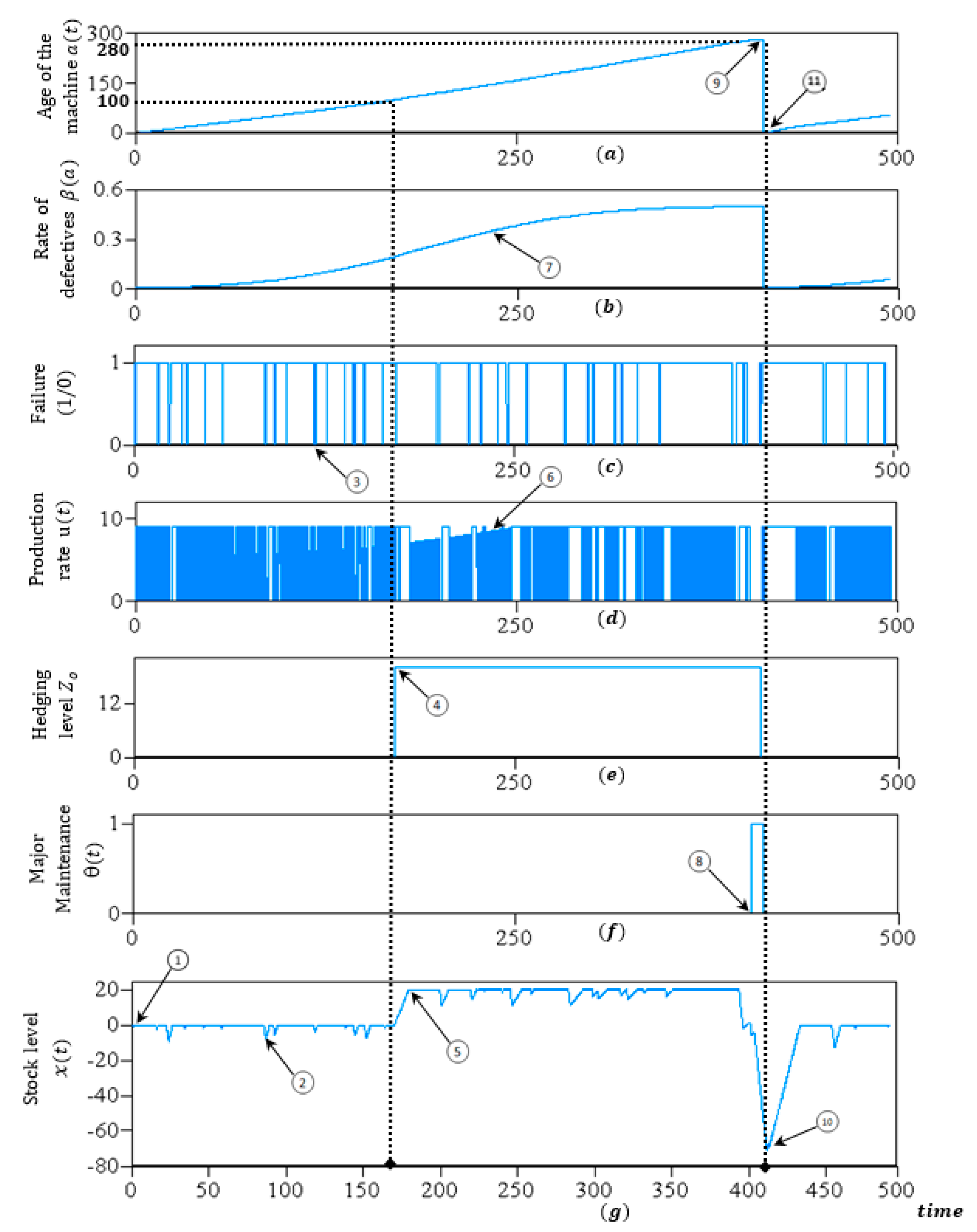
In order to ensure the accuracy of the simulation model, we conducted a validation analysis, where we traced a set of key indicators representative of the system behavior. In Figure 2, we present a simulation sample of the dynamics of the production system over a period of time where the control parameters were set to Z p = 20 , B J I T = 100 , and A 0 = 280 . From observing Figure 2, we note that at time t = 0 , the production unit is in brand-new conditions and so there is no need to maintain safety stock, thus Z p = 0 (see arrow 1 in Figure 2g). After that, we note the occurrence of several random failures, as in time t = 90 , where we see the reduction of the stock level when the unit fails (see arrow 2 in Figure 2g). Failures are identified in Figure 2c, as marked by arrow 3. Then, at time t = 160 , the unit reaches the critical age B J I T = 100 , which indicates the change of the production policy, triggering the increase of the stock level from Z p = 0 to Z p = 20 (see arrow 4 in Figure 2e). At this point ( t = 160 ), the stock level will progressively increase until its optimal threshold value Z p = 20 (see arrow 5 in Figure 2g). The change of the production threshold indicates that given the accumulated effects of deterioration on the machine, mainly observed in the increase of the rate of defectives, safety stock is needed to ensure demand satisfaction with flawless parts. As the machine continues its deterioration pattern, we note that at time t = 240 , the unit operates at rate d / ( 1 β ( a ) ) (see arrow 6 in Figure 2d) to compensate for the increase in the rate of defectives, since its level of deterioration is considerably high, as indicated by arrow 7 in Figure 2b. Then at time t = 400 , the unit reaches the critical age A 0 = 280 that triggers a major maintenance (see arrow 8 in Figure 2f). Before the conduction of such major maintenance, the production unit reaches its maximum level of deterioration, as noted by arrow 9 in Figure 2a. Additionally, we observe from arrow 10 in Figure 2g that the stock level decreases considerably, since the conduction of a major maintenance requires more time than a minimal repair. Furthermore, after the conduction of a major maintenance, we observe a considerable reduction in the rate of defectives, as shown by arrow 11 in Figure 2a. This is because major maintenance restores the production unit to AGAN conditions and eliminates the effects of deterioration. From this point, the production threshold is set again to Z p = 0 , indicating the beginning of a new deterioration cycle. Finally, based on the assessment of the dynamics of Figure 2, we verify that the production and major maintenance policies operate properly: A safety stock is needed when the age of the unit reaches the critical age B J I T , and a major maintenance is triggered when such age surpasses the value of A 0 .

5. Numerical Example

For illustrative purposes, this section provides a numerical example of the proposed integrated model. In this numerical instance, we considered three independent variables ( Z p , B J I T , A 0 ) and one dependent variable denoted by the total incurred cost. Simulation runs are conducted according to a complete 3 3 factorial design. For each combination of independent factors ( Z p , B J I T , A 0 ) , the design 3 3 is replicated four times, denoting ( 3 3 × 4 ) = 108 simulation runs. The simulation run length of each replication is set to 100,000 time units to ensure steady state conditions. The value of the parameters used in the numerical example are provided in Table 1.
Table 2 presents the costs parameters used in the numerical example.
The levels of the independent variables ( Z p , B J I T , A 0 ) , presented in Table 3, are chosen from the observation of the production unit given by preliminary runs made off-line. In what follows, to ensure that B J I T < A o , we define B J I T = k · A o , where k [ 0 , 1 ] .
Using the data of Table 1, Table 2 and Table 3, the proposed model collects simulation data to fit the dependent variable by a second-order regression function. The simulation results are handled using the statistical software STATGRAPHICS in order to conduct an analysis of variance (ANOVA) and validate the regression model obtained. In this case, the corresponding cost function is given as follows:
T C ( Z p , k , A 0 ) = 631.209 5.163 · Z 0 351.679 · k 2.00021 · A 0 + 0.0144789 · Z o 2 + 0.689607 · Z 0 k + 0.00763879 · Z 0 A 0 + 339.941 · k 2 + 0.322369 · k · A 0 + 0.00302754 · A o 2
Referring to the equation above, Table 4 presents the ANOVA analysis conducted. From this table, we note that all main factors, quadratic effects, and interactions are statistically significant for the response variable, since we note a P-value 5%. Furthermore, we observe a coefficient of correlation of R 2 = 0.902 . This value states that the second-order regression model (15) explains 90.20% of the variability observed in the total incurred cost.
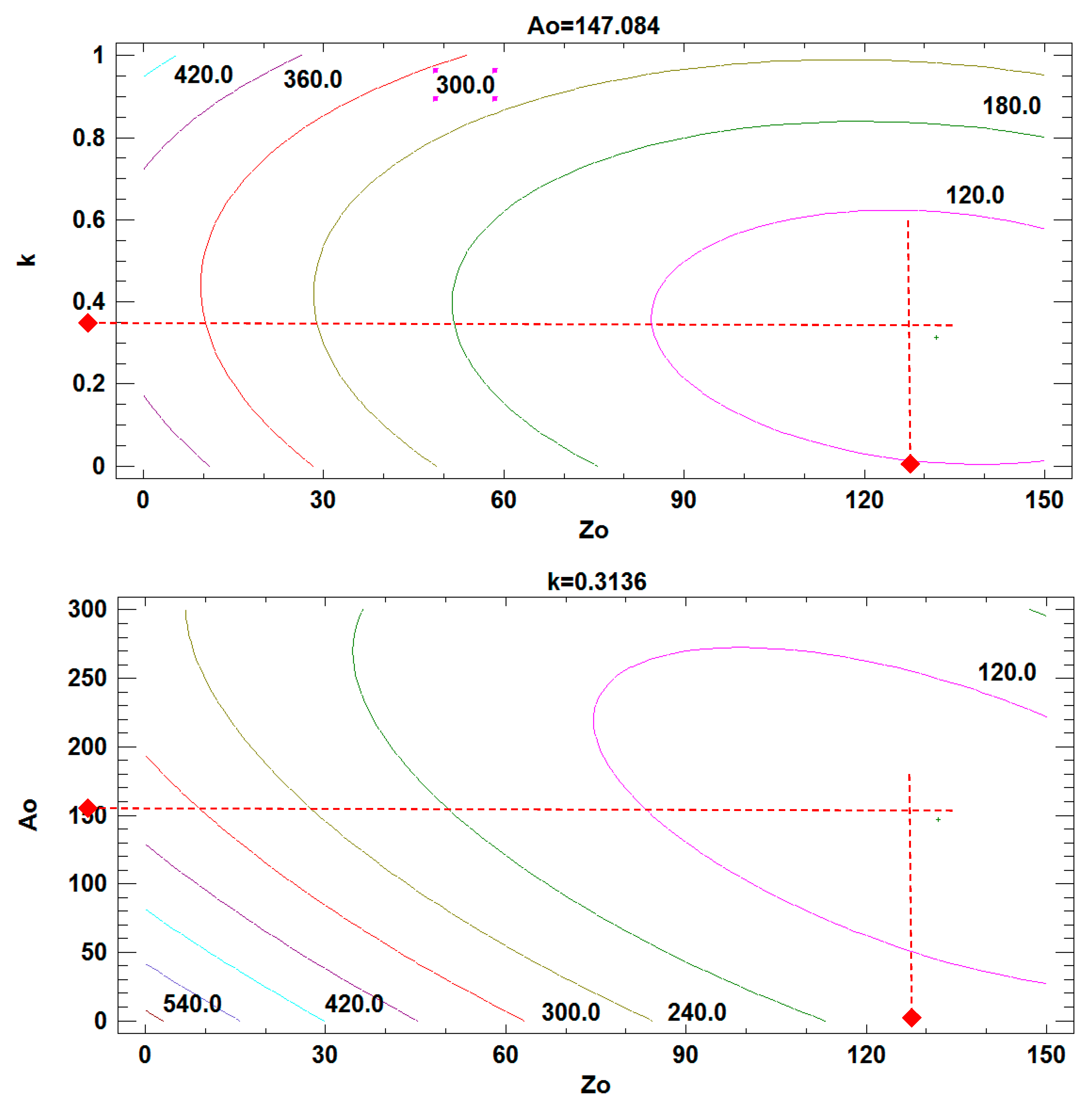
Figure 3 presents the projection of the cost regression model onto two-dimensional spaces.
For our numerical example, the obtained optimal solution is presented in Table 5. The value of k * = 0.3136 yields to define B J I T * = 46.12. The optimal values, presented in Table 5, are the recommended parameters which should be applied to jointly control the production rate and the major maintenance interventions.
From 50 extra-replications of the simulation model, we validated the optimal solution by verifying that the obtained total cost is within the confidence interval [85.69,91.22].

6. Sensitivity and Results Analysis

The primary objective of this section is to proceed with further analysis of a set of experiments and analyze the sensitivity of several cost parameters. The aim of the analysis is to study the behavior of the proposed integrated model, and compare the value of the control parameters and the total incurred cost for different system conditions derived from a basic case. Table 6 presents ten different configurations derived from the variation of five cost categories.
The obtained results of the sensitivity analysis are presented in Table 7, and can be interpreted as follows:
Variation of the inventory cost: When the inventory cost C + increases (case II), the proposed policy reacts by decreasing the production threshold Z p * , since the inventory of products is more penalized. With the increase of such penalization, we also notice that product inventory is limited to the bare minimum, and so the system extends the JIT policy for a longer period of time, thus increasing age B J I T * . By examining the results, we observe that the increment of C + promotes the conduction of more frequent major maintenance as a countermeasure to ensure the production of flawless units. Thus, at increasing C + , the critical age for major maintenance A 0 * reduces. When the inventory cost decreases, we note the opposite effects (case I).
Variation of the backlog cost: When the backlog cost increases (case IV), the shortages of products are more penalized, and thus the production threshold Z p * increases as a protection against the lack of product. Additionally, we note that product deficiency is also tackled by reducing the critical age B J I T * , and with this measure the unit applies less time the JIT policy, thus keeping product inventory for a longer period of time. Upon further investigation, the increment of the backlog cost exerts considerably more pressure to the unit performance, and hence major maintenance is conducted more frequently to mitigate the presence of defective units. The decrement of the backlog cost leads to the inverse effects (case III).
Variation of the minimal repair cost: With the increment of the repair cost C R (case VI), major maintenance must be performed more frequently, since the true usefulness of such maintenance is its ability to mitigate the presence of defective units, so the critical age A 0 * reduces. Furthermore, we note that at reducing age A 0 * , the unit will remain operational for less time, and thus the production threshold becomes less restricted, increasing Z p * as a countermeasure to ensure enough product availability to satisfy customers’ demand. Additionally, product availability is increased by reducing the period of time where the JIT policy is applied, since we note that at increasing C R , the critical age B J I T * reduces. When the repair cost decreases, we observe the inverse effects (case V).
Variation of the major maintenance cost: The increase of the major maintenance cost C M (case VIII) is expected to delay the conduction of major maintenance, thus increasing age A 0 * . This is because the production unit must attain higher levels of deterioration to justify the expensive cost of a major maintenance. Moreover, the intended consequence of delaying the major maintenance is that the unit will be operational for more time, increasing its responsiveness to customers’ demand, and also reducing the need for inventory, decreasing the production threshold Z p * . Furthermore, with more time available for production, the JIT policy is implemented for a longer period of time, and this increases age B J I T * . The reduction of the major maintenance cost has the inverse effects (case VII).
Variation of the defectives cost: When increasing the defectives cost C d e f (case X), it is logical to observe that major maintenances are conducted more frequently to restore the unit faster and, most importantly, reduce the amount of defective units that reach the final customer. Moreover, a close examination of the increment of C d e f shows that the system opts to increase the production threshold to ensure that customers are satisfied with flawless units. This previous measure is complemented with the reduction of the critical age B J I T * to limit the implementation of the JIT policy to a shorter period of time. With this measure, more inventory is available to replace defective units if necessary. The opposite occurs when the defective cost decreases (case IX).
The essence of the preceding analysis and the results of Table 7 is to illustrate the efficiency of our resolution approach and confirm that the structure of the proposed joint control policy remains during all the analysis.

7. Comparative Study

The final issue to be handled in this paper is the conduction of a comparative study which serves to highlight the potential cost savings that can be obtained from our joint control policy. In particular, we compare the performance of the integrated policy ( Z p , B J I T , A 0 ) , which we denoted as Policy-I, with an alternative policy in order to remark the advantage of implementing a JIT policy for moderate levels of deterioration. The second policy considered in the comparison is described as follows:
Policy-II: This paper is derived from the results of Bouslah et al. [30], where the production planning does not implement a JIT strategy. The production strategy consists only of the determination of an optimal inventory threshold level Z p o * , which is constant during the entire time horizon. In this Policy-II, the control parameter B J I T * is disregarded. The control parameters of Policy-II are then ( Z p , A 0 ) , which are jointly optimized.
Fundamentally, a simplified version of the optimization approach described in Section 4 is used to determine the optimal values of the control parameters ( Z p , A 0 ) for Policy-II. In this case, we use a two-factor experimental design for each combination of Z p and A 0 . A regression analysis was used to fit the total expected cost by a quadratic model, using the data of the basic case of Table 1 and Table 2, and the ANOVA for Policy-II reported R 2 = 0.8863 . Furthermore, the two design factors and their interactions were significant, obtaining the following quadratic function:
T C ( Z p , A 0 ) = 579.73 5.32303 · Z 0 1.79105 · A 0 + 0.0165384 · Z o 2 + 0.0088219 · Z 0 A 0 + 0.00231366 · A o 2
When minimizing Equation (16), the cost function for Policy-II provides the results presented in Table 8.
According to Policy-II, the production threshold Z 0 reduces when JIT policy is not implemented. In contrast, Policy-I reported a threshold Z 0 higher than in Policy-II, but the inventory level reaches Z 0 after the age of the machine surpasses B J I T * . Under Policy-II, the conduction of major maintenance is delayed, increasing the critical age A 0 * to compensate for the decrease of the production threshold. Herein, we note that a major difference between these policies is that Policy-I is 37.39% more economical than Policy-II. The significant gap between the costs of both policies is due to the fact that first, Policy-II generates extra inventory costs from implementing the production threshold Z 0 since the beginning of the considered time period. In contrast, Policy-I achieves important cost saving at implementing a JIT policy during the period of time when machine is almost in brand-new conditions. Second, the delay of major maintenances in Policy-II leads to extra defective costs due to the increase of the critical age A 0 * . The obtained results of Table 8 confirm key advantages of our proposed control policy.

8. Conclusions

The practical implications of simultaneously addressing production, product quality, and maintenance strategies for deteriorating production systems are immense. The proposed new model contributes to the active field of research that studies the interactions of production, quality, and maintenance in four ways. First, the strong interrelations of the three key functions of production, quality, and maintenance were fully considered in the proposed joint control policy. Second, we demonstrated through numerical instances that the deterioration process has a direct effect on the production and maintenance policy, since the optimal control parameters of such policies are determined in function of the level of deterioration of the machine. Third, we have found that a JIT policy can be implemented before an optimal age B J I T * , under which the production unit is considered to operate in brand-new conditions, where the effects of the deterioration process are so negligible that there is no need to maintain products in stock. Another important contribution of this paper is that the maintenance strategy is based on quality information feedback that exploits the link between the level of deterioration of the unit and the amount of defectives that it produces. Quality information can be easily determined by the rate of defectives and interpreted to determine the appropriate maintenance option. The integrated model proposed in this paper can be applied for stochastic production systems subject to quality deterioration and where maintenance strategies are available to cope with such effects. Managerial implications for implementing our integrated model in practice require real-time visibility of the process conditions. In this case, for an appropriate control of operations, it is necessary to know the level of product inventory and the level of product quality. Furthermore, product quality should be properly supervised to monitor the production unit and determine an efficient schedule for major maintenance. The sensitivity analysis and the comparative study conducted serve to highlight the efficiency of our control policy compared with alternative strategies that disregard the implementation of JIT polices in the production strategy. The critical point is that considerable cost savings could be obtained from implementing our joint control policy. One limitation of our paper is to assume that the rate of defectives is known all the time. However, an inspection sampling plan could be implemented instead of our approach. In summary, the results obtained so far are satisfactory and foster further research into this domain. A possible extension of this paper is the consideration of more sophisticated sampling plans in the quality control policy, such as the CSP-1 plan or multiple sampling plans.

Author Contributions

H.R.-G. and O.M.-A. conceived the mathematical model; J.R.C.-A. and J.G.-G. developed the numerical approach; A.O.O.-R. performed the sensitivity analysis; and G.E.A.-F. conducted the comparative study.

Funding

This research received no external funding.

Conflicts of Interest

The authors declare no conflict of interest.

References

  1. Kim, J.; Gershwin, S.B. Integrated quality and quantity modeling of a production line. OR Spectr. 2005, 27, 287–314. [Google Scholar] [CrossRef] [Green Version]
  2. Kim, J.; Gershwin, S.B. Analysis of long flow lines with quality and operational failures. IIE Trans. 2008, 40, 284–296. [Google Scholar] [CrossRef] [Green Version]
  3. Colledani, M.; Tolio, T. Integrated analysis of quality and production logistics performance in manufacturing lines. Int. J. Prod. Res. 2011, 49, 485–518. [Google Scholar] [CrossRef] [Green Version]
  4. Colledani, M.; Ebrahimi, D.; Tolio, T. Integrated quality and production logistics modelling for the design of selective and adaptive assembly systems. CIRP Ann. Manuf. Technol. 2014, 63, 453–456. [Google Scholar] [CrossRef]
  5. Hajji, A.; Mhada, F.; Gharbi, A.; Pellerin, R.; Malhamé, R. Integrated product specifications and productivity decision making in unreliable manufacturing systems. Int. J. Prod. Econ. 2011, 129, 32–42. [Google Scholar] [CrossRef] [Green Version]
  6. Bouslah, B.; Gharbi, A.; Pellerin, R. Joint optimal lot sizing and production control policy in an unreliable and imperfect manufacturing system. Int. J. Prod. Econ. 2013, 144, 143–156. [Google Scholar] [CrossRef] [Green Version]
  7. Mhada, F.; Malhamé, R.; Pellerin, R. Joint assignment of buffer sizes and inspection points in unreliable transfer lines with scrapping of defective parts. Prod. Manuf. Res. 2013, 1, 79–101. [Google Scholar] [CrossRef]
  8. Rivera-Gómez, H.; Lara, J.; Montaño-Arango, O.; Hernández-Gress, E.S.; Corona-Armenta, J.R.; Santana-Robles, F. Joint production and repair efficiency planning of a multiple deteriorating system. Flex. Serv. Manuf. J. 2018. [Google Scholar] [CrossRef]
  9. Kumar-Sharma, R.; Kumar, D.; Kumar, P.F.M. A pragmatic tool to model, analyse and predict complex behavior of industrial systems. Eng. Comput. 2007, 24, 319–345. [Google Scholar] [CrossRef]
  10. Hajej, Z.; Turki, S.; Rezg, N. Modelling and analysis for sequentially optimizing production, maintenance and delivery activities taking into account product returns. Int. J. Prod. Res. 2015, 53, 4694–4719. [Google Scholar] [CrossRef]
  11. Nourelfath, M.; Nahas, N.; Ben-Daya, M. Integrated preventive maintenance and production decisions for imperfect processes. Reliab. Eng. Syst. Saf. 2016, 148, 21–31. [Google Scholar] [CrossRef]
  12. Dellagi, S.; Chelbi, A.; Trabelsi, W. Joint integrated production-maintenance policy with production plan smoothing through production rate control. J. Manuf. Syst. 2017, 42, 262–270. [Google Scholar] [CrossRef]
  13. Callahan, R.; Hubbard, K.; Strong, S. Computational methods for planning and developing flexible manufacturing systems. Eng. Comput. 2007, 22, 958–971. [Google Scholar] [CrossRef]
  14. Dehayem Nodem, F.; Kenné, J.P.; Gharbi, A. Simultaneous control of production, repair/replacement and preventive maintenance of deteriorating manufacturing systems. Int. J. Prod. Econ. 2011, 134, 271–282. [Google Scholar] [CrossRef] [Green Version]
  15. Hajej, Z.; Dellagi, S.; Nidhal, R. Optimal integrated maintenance/production policy for randomly failing systems with variable failure rate. Int. J. Prod. Res. 2011, 49, 5695–5712. [Google Scholar] [CrossRef]
  16. Khatab, A.; Ait-Kadi, D.; Rezg, N. Availability optimization for stochastic degrading systems under imperfect preventive maintenance. Int. J. Prod. Res. 2011, 52, 4132–4141. [Google Scholar] [CrossRef]
  17. Ayed, S.; Hajej, Z.; Turki, S.; Rezg, N. FPA method for optimal production planning under availability/degradation machine and subcontracting constraint. Int. J. Prod. Res. 2017, 55, 2135–2148. [Google Scholar] [CrossRef]
  18. Gharbi, A.; Hajji, A.; Dhouib, K. Production rate control of an unreliable manufacturing cell with adjustable capacity. Int. J. Prod. Res. 2011, 49, 6539–6557. [Google Scholar] [CrossRef] [Green Version]
  19. Berthaut, F.; Gharbi, A.; Dhouib, K. Joint modified block replacement and production/inventory control policy for a failure-prone manufacturing cell. Omega 2011, 39, 642–654. [Google Scholar] [CrossRef] [Green Version]
  20. Hlioui, R.; Gharbi, A.; Hajji, A. Integrated quality strategy in production and raw material replenishment in a manufacturing-oriented supply chain. Int. J. Adv. Manuf. Technol. 2015, 81, 335–348. [Google Scholar] [CrossRef] [Green Version]
  21. Tolio, T.; Ratti, A. Performance evaluation of two-machine lines with generalized thresholds. Int. J. Prod. Res. 2018, 56, 926–949. [Google Scholar] [CrossRef]
  22. Green, K.W., Jr.; Inman, R.A.; Birou, L.M.; Whitten, D. Total JIT (T-JIT) and its impact on supply chain competency and organizational performance. Int. J. Prod. Econ. 2014, 147, 125–135. [Google Scholar] [CrossRef]
  23. Fullerton, R.; McWatters, C. The production performance benefits from JIT implementation. J. Oper. Manag. 2001, 19, 81–96. [Google Scholar] [CrossRef]
  24. Alcaraz, J.L.; Macías, A.A.; Luevano, D.J.; Fernández, J.B.; López, A.D.; Macías, E.J. Main benefits obtained from a successful JIT implementation. Int. J. Adv. Manuf. Technol. 2016, 86, 2711–2722. [Google Scholar] [CrossRef]
  25. Kouedeu, A.F.; Kenne, J.P.; Dejax, P.; Songmene, V.; Polotski, V. Production and maintenance planning for a failure-prone deteriorating manufacturing system: A hierarchical control approach. Int. J. Adv. Manuf. Tech. 2016, 76, 1607–1619. [Google Scholar] [CrossRef]
  26. Amendola, L.; Artacho-Ramirez, M.A.; Depool, T. Analysis of key factors to improve maintenance management in the oil & gas industry in latin america. DYNA Ing. Ind. 2017, 92, 567–571. [Google Scholar] [CrossRef]
  27. Rivera-Gómez, H.; Gharbi, A.; Kenné, J.P.; Montaño-Arango, O.; Hernández-Gress, E.S. Subcontracting strategies with production and maintenance policies for a manufacturing system subject to progressive deterioration. Int. J. Prod. Econ. 2018, 200, 103–118. [Google Scholar] [CrossRef]
  28. Goti, A.; Oyarbide-Zubillaga, A.; Sánchez, A. Optimizing preventive maintenance by combining discrete event simulation and genetic algorithms. Hydrocarb. Process. 2007, 86, 115–122. [Google Scholar]
  29. Oyarbide-Zubillaga, A.; Goti, A.; Sanchez, A. Preventive maintenance optimization of multi-equipment manufacturing systems by combining discrete event simulation and multi-objective evolutionary algorithms. Prod. Plan. Control 2008, 19, 342–355. [Google Scholar] [CrossRef]
  30. Bouslah, B.; Gharbi, A.; Pellerin, R. Joint production, quality and maintenance control of a two-machine line subject to operation-dependent and quality-dependent failures. Int. J. Prod. Econ. 2018, 195, 210–226. [Google Scholar] [CrossRef]
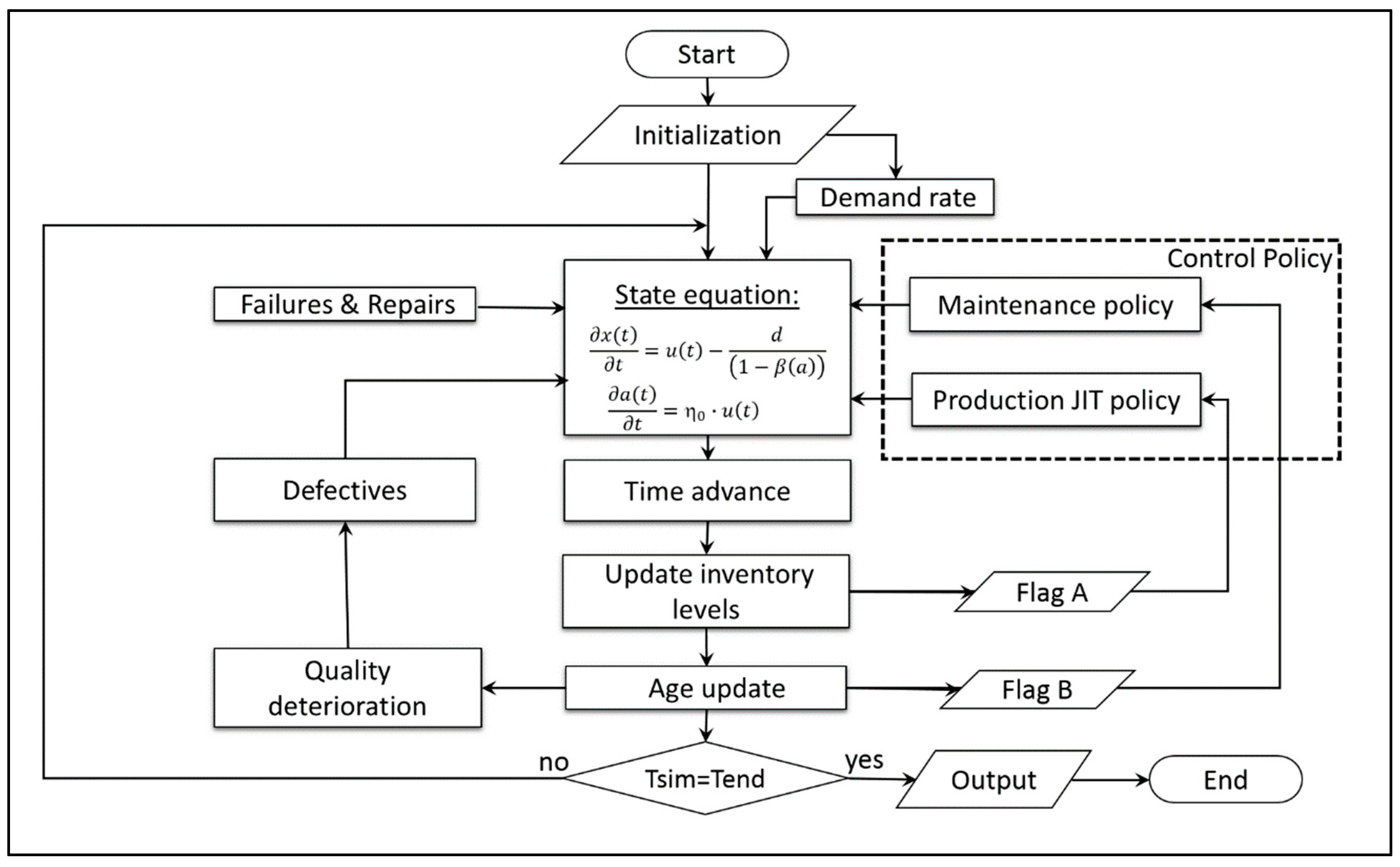
Figure 1. Block diagram of the simulation model.
Applsci 09 01180 g001
Figure 2. Validation of the simulation model.
Applsci 09 01180 g002
Figure 3. Cost projection of the estimated expected total cost.
Applsci 09 01180 g003
Table 1. Parameters for the numerical example.
Parameter: q 12
(1/time units)
q 21
(1/time units)
q 13
(1/time units)
q 31
(1/time units)
θ
Value:0.11.550.150.08
Parameter: u m a x
(product/time units)
d
(product/time units)
η 0 b 0 b 1
Value:95.50.10.010.49
Parameter: η 1 η 2
Value:15 × 10−6.22.4
Table 2. Cost parameters for the numerical example.
Parameter: C + ($/Products/Time Units) C ($/Products/Time Units) C R ($/Repair) C M ($/Major Intervention) C d e f ($/Product)
Value:150100300020
Table 3. Cost parameters for the statistical analysis.
FactorLow LevelHigh LevelDescription
Z 0 10150Production threshold
k 0.10.9Critical value for increasing the stock level to Z p
A o 40300Critical age for triggering major maintenance
Table 4. ANOVA table.
SourceSum of SquaresDfMean SquareF-RatioP-Value
A:Zo255,280.01255,280.0154.070.0000
B:k55,583.3155,583.333.550.0000
C:Ao23,986.3123,986.314.480.0004
AA60,400.7160,400.736.450.0000
AB8,948.118,948.15.400.0249
AC115,969.01115,969.069.990.0000
BB35,500.0135,500.021.430.0000
BC6,744.1216,744.124.070.0499
CC31,414.9131,414.918.960.0001
blocks1,348.0211,348.020.810.3721
Total error71,248.0431,656.93
Total (corr.)666,423.053
Table 5. Optimal control parameters and cross-check validation.
Z 0 * k * A 0 * Total Cost EstimateCross-Check Confidence Interval (95%)
Factor132.020.3136147.08488.13 [ 85.69 ,   91.22 ]
Table 6. Sensitivity analysis for different cost variations.
Cost Variations
CasesCost Parameter C + C C R C M C d e f
Basic case150100300020
Case I C + 0.525100300020
Case II 2150100300020
Case III C 120100300020
Case IV 170100300020
Case V C R 15020300020
Case VI 150300300020
Case VII C M 150100100020
Case VIII 150100500020
Case IX C d e f 15010030005
Case X 150100300050
Table 7. Sensitivity analysis for different cost variations.
Control Parameters VariationsTotal Cost Variations
Par.Cases Z p * k * B J I T * A 0 * C * Remark
-Basic case132.040.313646.12147.0888.13Base for the comparison
C + Case I140.840.197829.63149.8355.78 Z 0 * ,   B J I T * ,   A 0 *
Case II122.170.467066.32142.03133.08 Z 0 * ,   B J I T * ,   A 0 *
C Case III117.520.521578.19149.95 82.70 Z 0 * ,   B J I T * ,   A 0 *
Case IV136.920.250936.87146.98109.89 Z 0 * ,   B J I T * ,   A 0 *
C R Case V131.880.313546.28147.6580.88 Z 0 * ,   B J I T * ,   A 0 *
Case VI132.050.313745.67145.60106.28 Z 0 * ,   B J I T * ,   A 0 *
C M Case VII139.400.317837.13116.8577.63 Z 0 * ,   B J I T * ,   A 0 *
Case VIII127.250.311051.80166.5896.27 Z 0 * ,   B J I T * ,   A 0 *
C d e f Case IX126.580.307851.74168.1175.58 Z 0 * ,   B J I T * ,   A 0 *
Case X143.990.325632.74100.56107.35 Z 0 * ,   B J I T * ,   A 0 *
Table 8. Cost difference of the comparative study.
Control ParametersTotal
Cost *
Cost Difference Δ-Cost (%)
Description Z p o * B J I T * A 0 *
Policy-I132.0246.12147.0888.13-
Policy-II117.38-163.26121.09+37.39%