The Evolving Value of Photovoltaic Module Efficiency


1
Bloomberg L.P., San Francisco, CA 94111, USA
2
School for the Future of Innovation in Society, Arizona State University, Tempe, AZ 85287, USA
*
Author to whom correspondence should be addressed.
Appl. Sci. 2019, 9(6), 1227; https://doi.org/10.3390/app9061227
Submission received: 19 February 2019
/
Revised: 14 March 2019
/
Accepted: 18 March 2019
/
Published: 23 March 2019
(This article belongs to the Special Issue Next Generation Photovoltaic Solar Cells)
Abstract
:PV research is making efforts to create new cell and module efficiency records, while the manufacturing industry and the downstream project developers want to choose the optimal efficiency point where the best economics can be achieved at the system level. In this paper, we define representative system cost structurers for various applications in 2018 and quantify the value of greater module efficiency in lowering the levelized cost of electricity (LCOE). With the transparent methodology, we also extended the analysis into the future until 2025. As the value of module efficiency resides in non-module costs and the non-module costs will account for a higher percentage for a PV system in the future, industry will develop stronger motivation to adopt more efficient modules. Specifically, we examined the economics of bifacial modules and forecast that its market share would grow from 3% in 2018 to 40% in 2025.
1. PV to Supply 24% Electricity by 2050
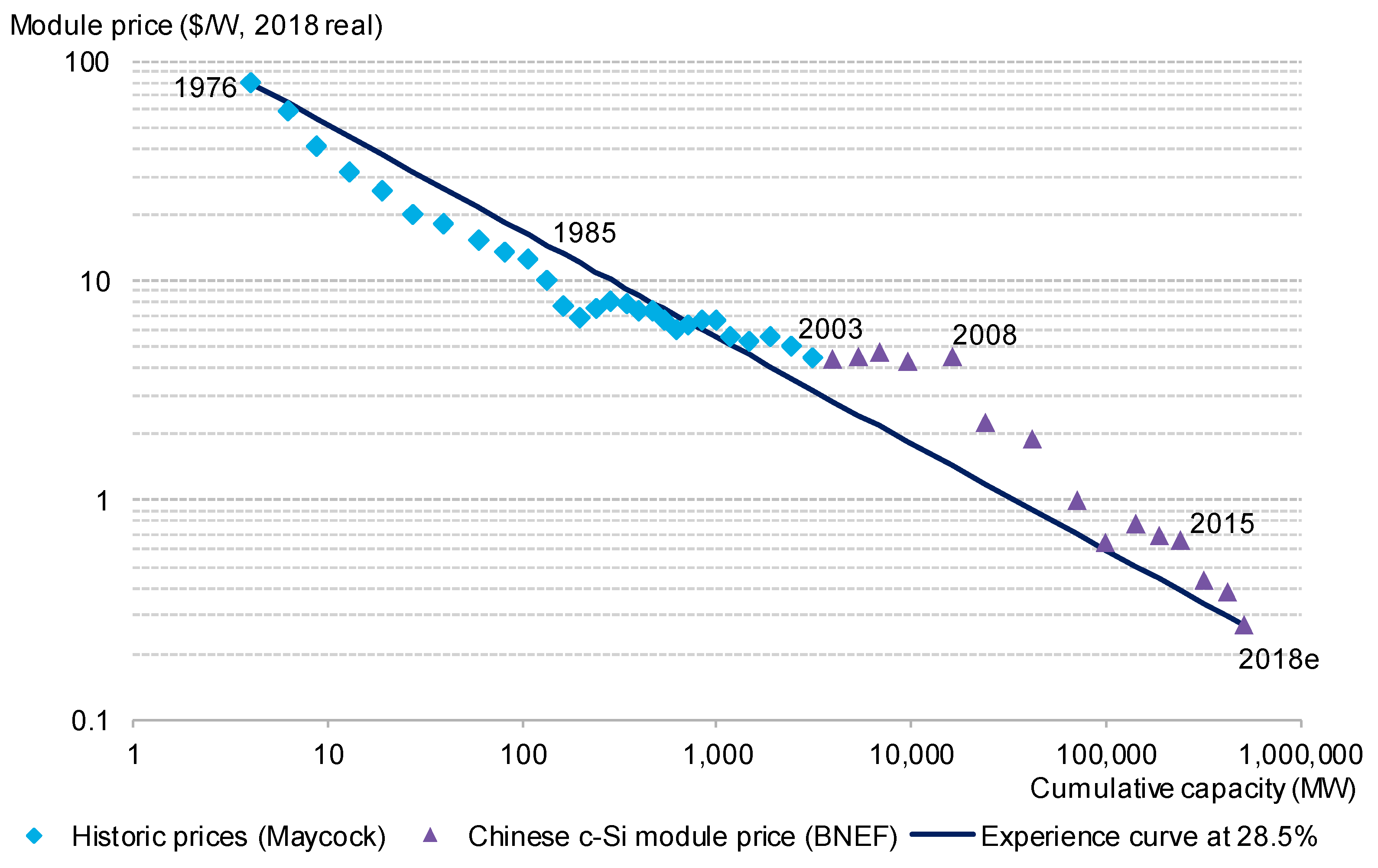
During the past 42 years (since 1976), PV module price dropped by 99.6% from $79.3/W to $0.3/W (both in 2018 USD), demonstrating a learning rate of 28.5% (Figure 1, [1]).
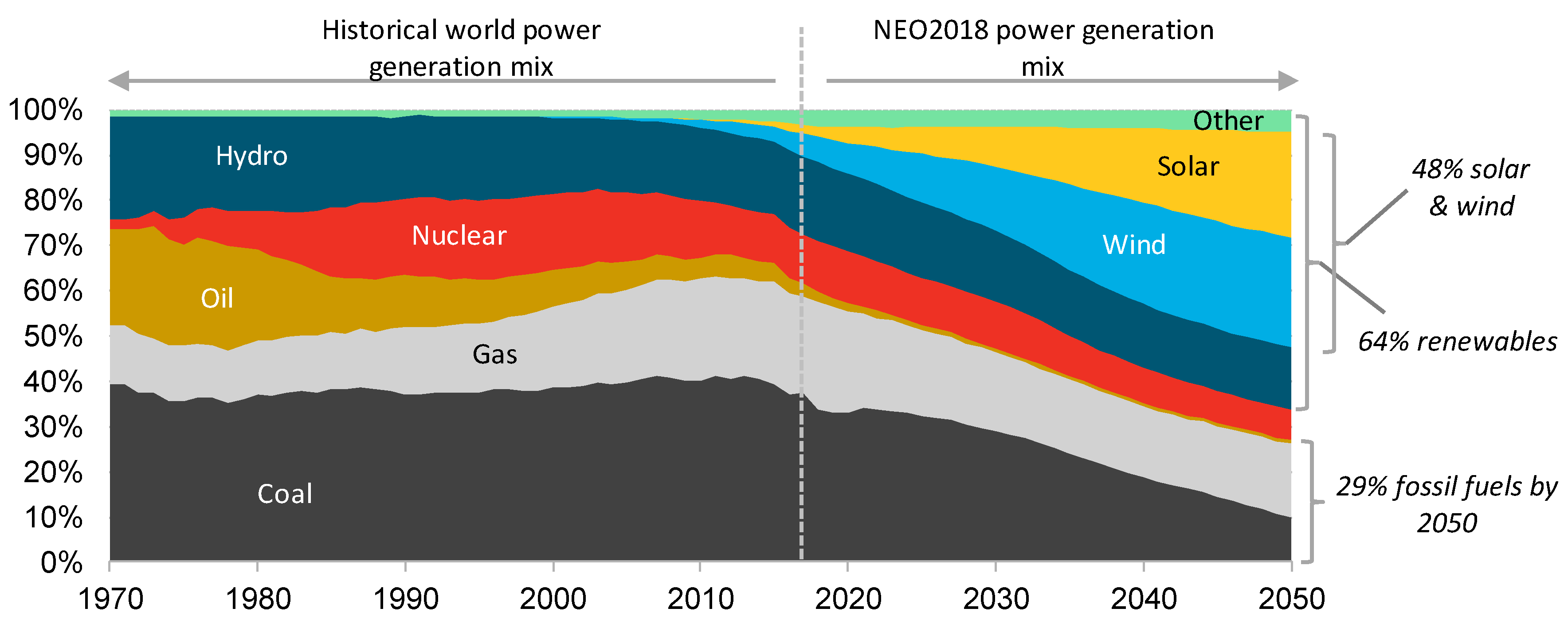
Along with the cost reduction of other components in PV systems, the economics of PV electricity has significantly improved. BloombergNEF expects 24% of worldwide electricity consumption will be supplied by PV by 2050, when a total of about 7TW PV will be installed (Figure 2, [2]).
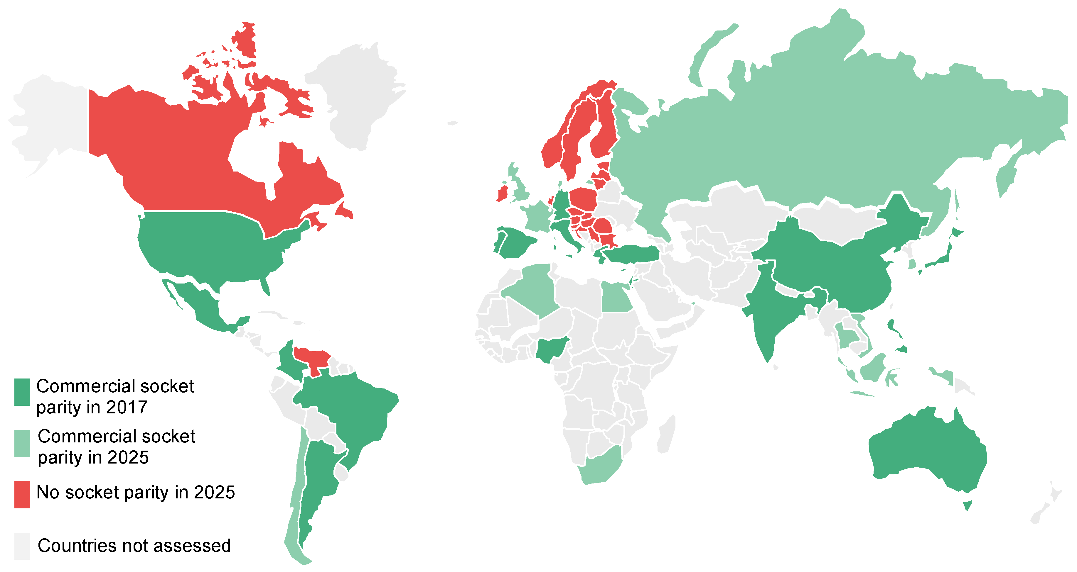
Despite the great potential of PV generation, continuous improvement is still needed before subsidies are eliminated. In industry, the ‘grid parity’ or ‘socket parity’ is defined by comparing the levelized cost of electricity (LCOE, to be defined) of PV generation and local retail price. For behind-the-meter applications—for example, commercial PV projects—the realized value of PV generation depends on the flow of the electricity, unless net metering policy is applied. This is because exported energy (uploaded to the grid) is usually valued at much lower rates than the retail rates. Figure 3 shows the commercial socket parity achievement without generation-based subsidies by country in 2017 and expectation for 2025, assuming 75% on-site consumption ([3]). Although socket parity will spread to more countries by 2025, there are still regions where subsidies are required to boost local market development. More analysis on residential socket parity can be found in the literature [3,4].
In addition to further efforts to lower the unit electricity cost, PV also needs to have its intermittency addressed in order to realize deeper penetration compared with the 2% contribution in power system in 2018 (Figure 2). The coupling between PV and storage (PVS) is becoming an emerging market, thanks to cheaper lithium-ion batteries and the cost savings from synergy between PV and storage in the integrated system design. This point is mentioned here to provide a general and complete view of PV development. However, it is not the focus of this paper. More details about PVS can be found in the literature [5,6].
While there are still many challenges for PV to conquer before it can become a significant contributor to global electricity generation, we focus on one specific topic: how higher module efficiency can lower PV LCOE.
2. The Value of Module Efficiency Resides in Non-Module Costs
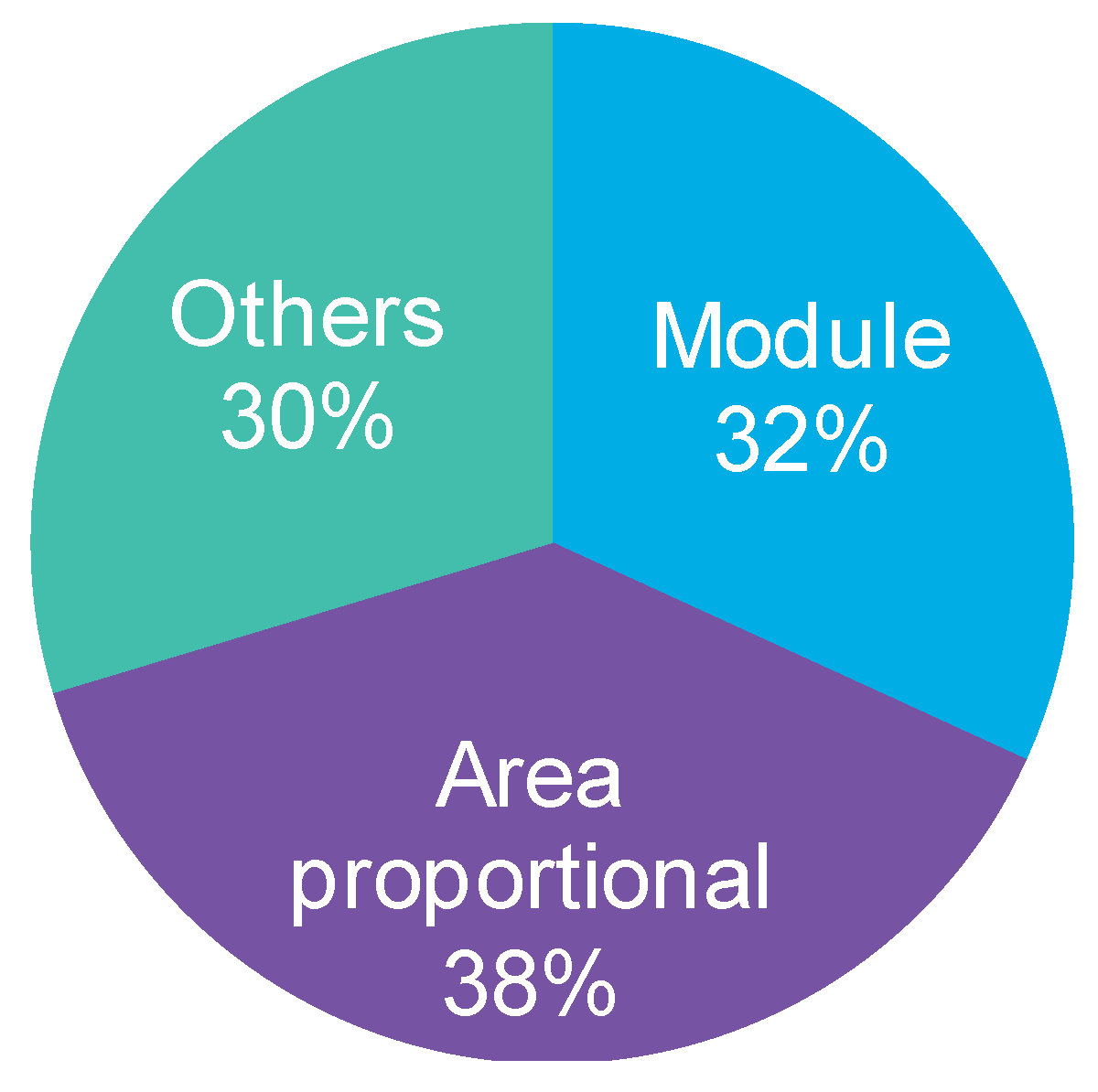
PV modules of higher efficiencies enjoy price premiums because they help lower the unit cost (per watt) of non-module components in a PV system. There are various ways of categorizing the costs of a PV project. Figure 4 shows a simple structure of a utility PV project’s cost to illustrate the value of module efficiency. The category referred to as ‘area-proportional’ includes spending on racking, land, construction, transportation, etc. ‘Others’ refers to costs of electronic components that are quoted in terms of power rather than area, and soft costs related to administration, due diligence, etc.
In a case with a restricted grid interconnection capacity or a defined project power capacity, when modules of a higher efficiency are adopted, the required number of modules, land area, and ‘area-proportional’ costs are all reduced linearly. Therefore, the per-watt spending on area-related items is inversely proportional to module efficiency. In a case with a defined land area, when modules of a higher efficiency are adopted, all area-proportional costs are averaged over more power, so their per-watt value is reduced proportionally. Additionally, some soft costs categorized as ‘others’ remain the same or increase only marginally. Depending on the specific correlation between a certain cost item in ‘others’ and the system power, the impact of module efficiency on ‘others’ varies. For illustration purpose, we set a simplified assumption that half of the ‘others’, or 15% of the system cost, is of a fixed value. The left-hand chart in Figure 5 shows the sensitivity of the non-module unit cost to module efficiency for the two scenarios. The impact of module efficiency is stronger when land area is restricted. Therefore, the maximum module price premium allowed is higher in such a case, as shown in the right-hand chart in Figure 5. The maximum allowed module price premium is derived, assuming the system unit capex is the same as the reference point, which corresponds to 17.7% module efficiency.
3. The Value of Module Efficiency Depends on System Cost Structure
The quantitative conclusion in the previous section is only valid for the cost structure shown in Figure 4. The value of module efficiency depends on the percentage of area-proportional non-module costs, and that of the fixed costs insensitive to project area or capacity. With the benchmark system costs in 2018 categorized by function, defined by BloombergNEF [7], we re-group them based on the correlation to area and power. Note that each project has a different cost dependence, and the values shown in Figure 6 are estimated for illustrative analysis purposes. (Prior to this paper, the same authors published one piece eight years ago, also to explore the value of module efficiency, with the benchmark system cost structure derived based on the market at that time [8].)
Different electricity generation technologies have diverse patterns for both expenditure and yield over time. A well-recognized metric to quantify the economics of a certain technology is levelized cost of electricity (LCOE), which is “the cost that, if assigned to every unit of energy produced (or saved) by the system over the analysis period, will equal the total life-cycle cost (TLCC) when discounted back to the base year” [9]. LCOE can be calculated using the following formula:
where Cn is the cost for year n, Qn is the energy output for the year n, d is the discount rate, and N is the analysis period. The parameters for all equations in this paper are summarized in Appendix A.
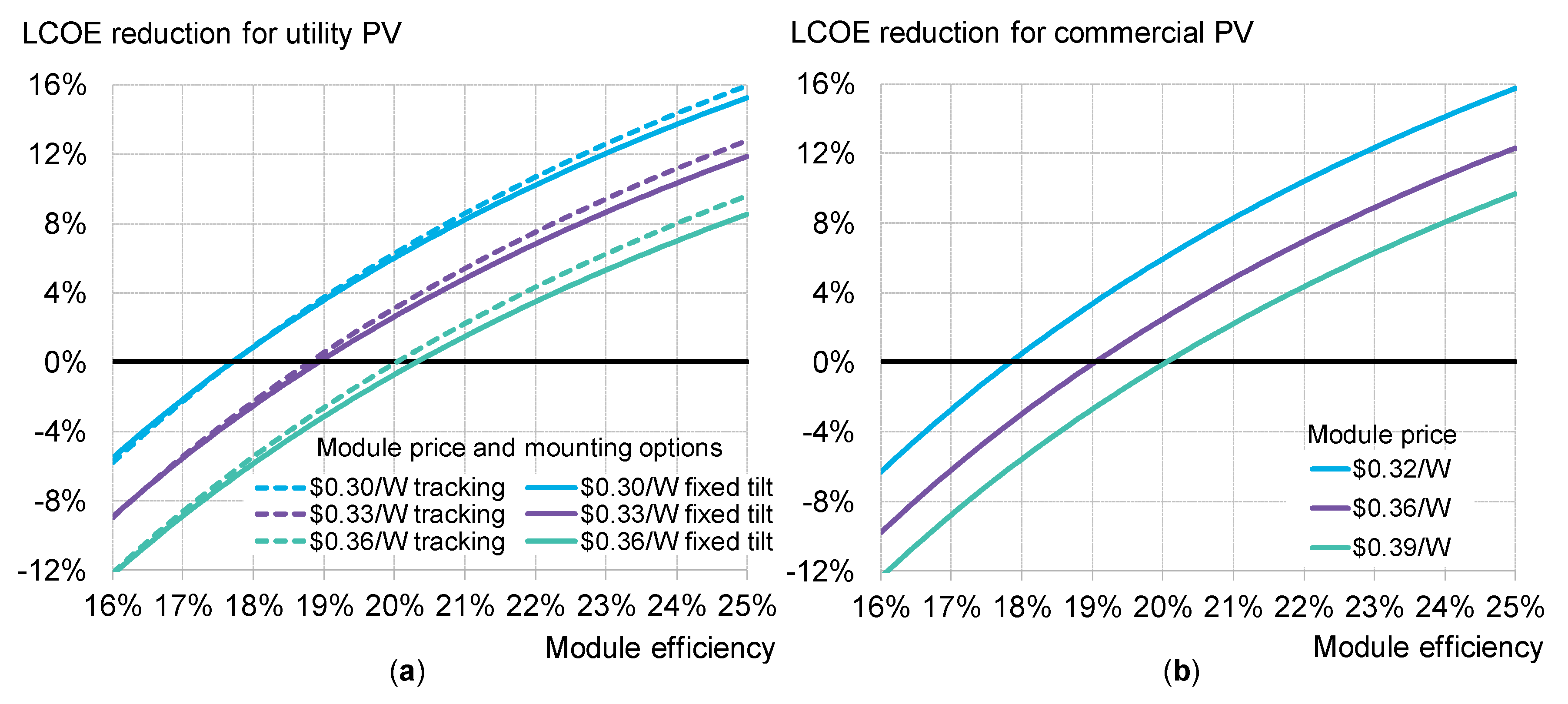
In this paper, we analyze the impact of module efficiency on system LCOE for three system configurations, as shown in Figure 6: utility with fixed tilt for modules, utility with one-axis tracking, and commercial projects with fixed tilt for modules. Assuming modules of different efficiencies will have the same per-watt yield, and operation cost is a fixed percentage of the system capital expenditure (capex), a PV project’s LCOE is proportional to the system unit capex. Applying the capex structure shown in Figure 6, we derive the impact of module efficiency and price on PV LCOE for different applications, in the ‘fixed-area’ scenario. In Figure 7, negative values on the y-axis suggest that LCOE in a certain scenario is higher than that in the reference case. For utility PV, when trackers are introduced, the proportion of area-proportional costs is a higher percentage of the total system capex, so module efficiency can impose stronger leverage in reducing system LCOE. This is reflected in the higher position of the dashed lines than the solid lines in the left-hand chart of Figure 7.
In commercial PV, due to restricted economies of scale, area-proportional and fixed non-module costs are higher than in utility PV. Module efficiency therefore holds more value in commercial PV. For instance, in a tracking utility PV, 20% efficient modules can ask for a price of $0.36/W (the intersection between the dashed green line and the black line in Figure 7a). In contrast, the same modules can push the quote up to $0.39/W in commercial PV (the intersection between the green line and the black line in Figure 7b).
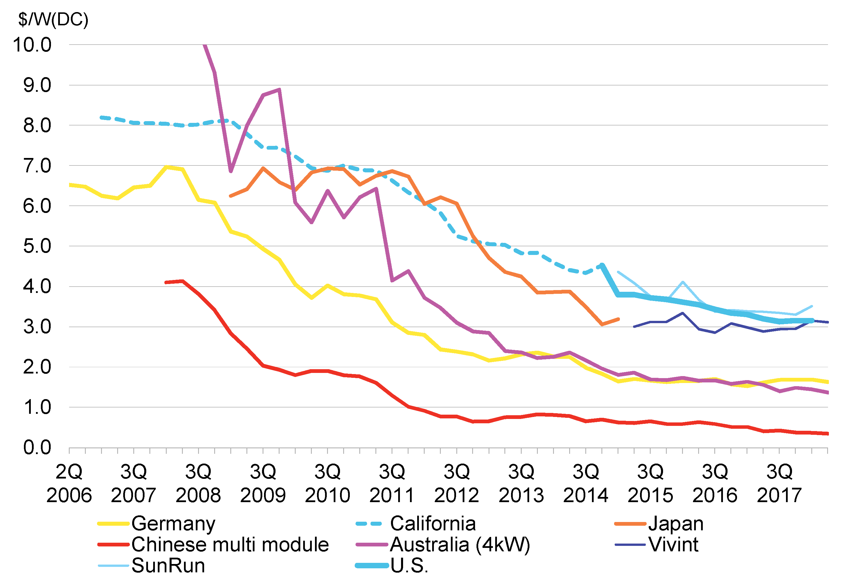
In general, the proportion of area-related and fixed costs in residential PV is greater than that in commercial PV, due to higher prices of equipment, labor, and process under the retail business model. However, the value heavily depends on the local market, as indicated by the wide range of residential system costs in Figure 8 [7]. The USA and Japan are the two most expensive residential PV markets, and the most popular markets for n-type modules. In the fourth quarter of 2018, p-type modules are quoted in the range of $0.35–0.40/W to U.S. utility developers, including transportation and tariffs, while n-type module suppliers sell for $0.65–0.75/W to U.S. distributors, who add about additional 10% margins in the final sales to residential PV owners [10].
Note that the cost structure presented in Figure 6 is considered representative of mature markets and no penalty tariffs on imported PV equipment are considered. The U.S. National Renewable Energy Laboratory (NREL) has updated the benchmark cost structure in 2018 for the domestic market, including antidumping tariffs and other impacts from various trade barriers [11].
In this paper, we address the impact of module efficiency on mainstream PV applications, which adopt crystalline silicon (c-Si) modules and either fixed-tilt or one-axis (more specifically, one-axis horizontal) tracking configurations. Additional discussion of other types of modules and tracking options is given in the last section of this paper. Other researchers have provided overviews of the value of various modules [12,13].
4. The Evolving Value of Module Efficiency
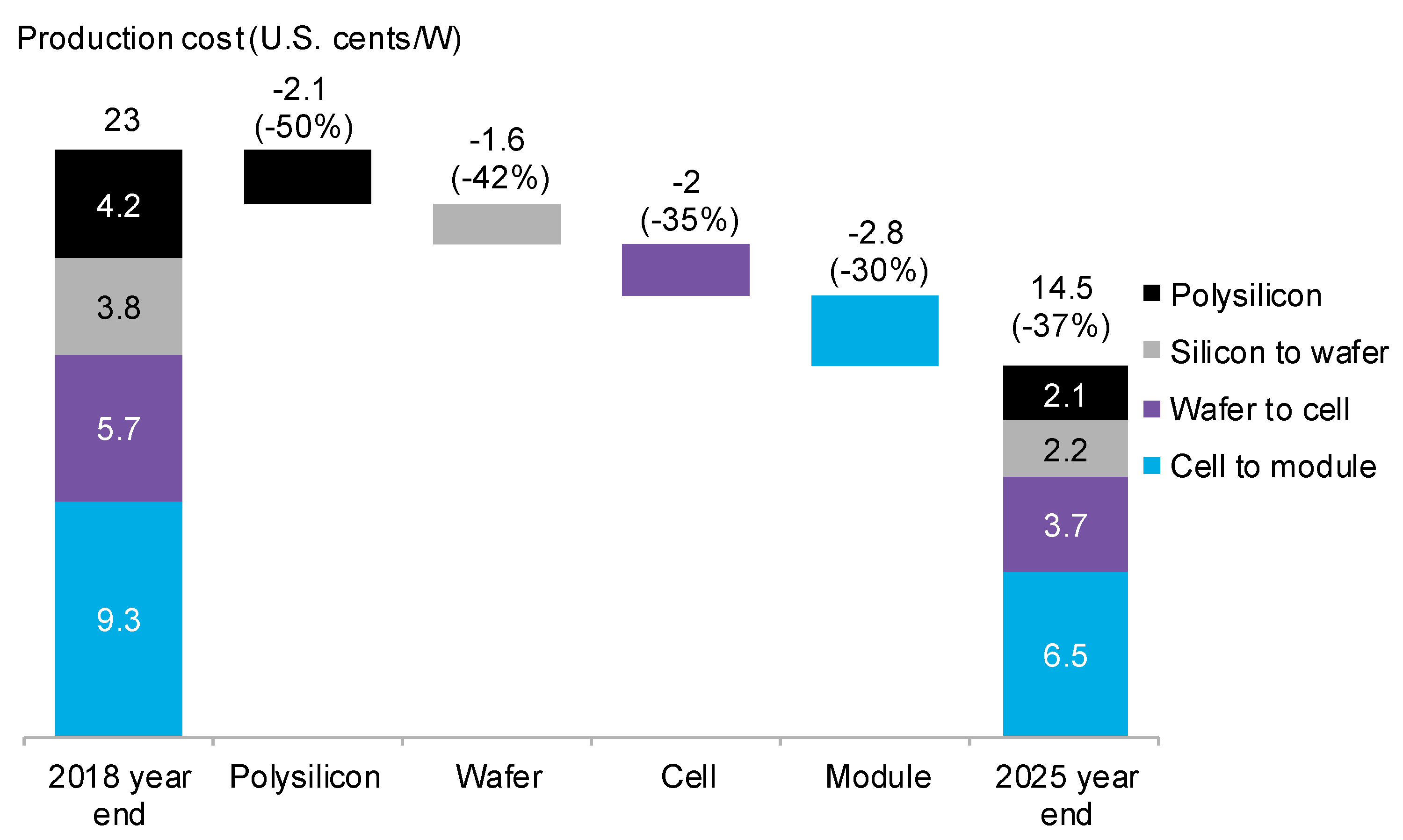
Module price will drop much faster than other system components in the coming years, due to sustainable technology innovation, continuous oversupply, and the choice of polysilicon makers to move to regions with low electricity rates [14]. Based on the forecast made by BloombergNEF, the best-case integrated module production cost will fall from $0.23/W at the end of 2018 to $0.145/W by 2025 [1], as shown in Figure 9.
While the module price fall will continue following a learning rate of 28.5%, we expect the industry average module efficiency to rise by 2.5% relatively, on an annual average basis. For utility PV projects with fixed tilt, BloombergNEF expects that the per DC watt system capex will drop by 33% by 2025, compared with 2018 [7]. The rate is 32% for commercial PV. We estimated the correlation between different cost components and area or power, and regrouped the spending, based on which the percentages of area-proportional costs and fixed costs are derived, as shown in Figure 10.
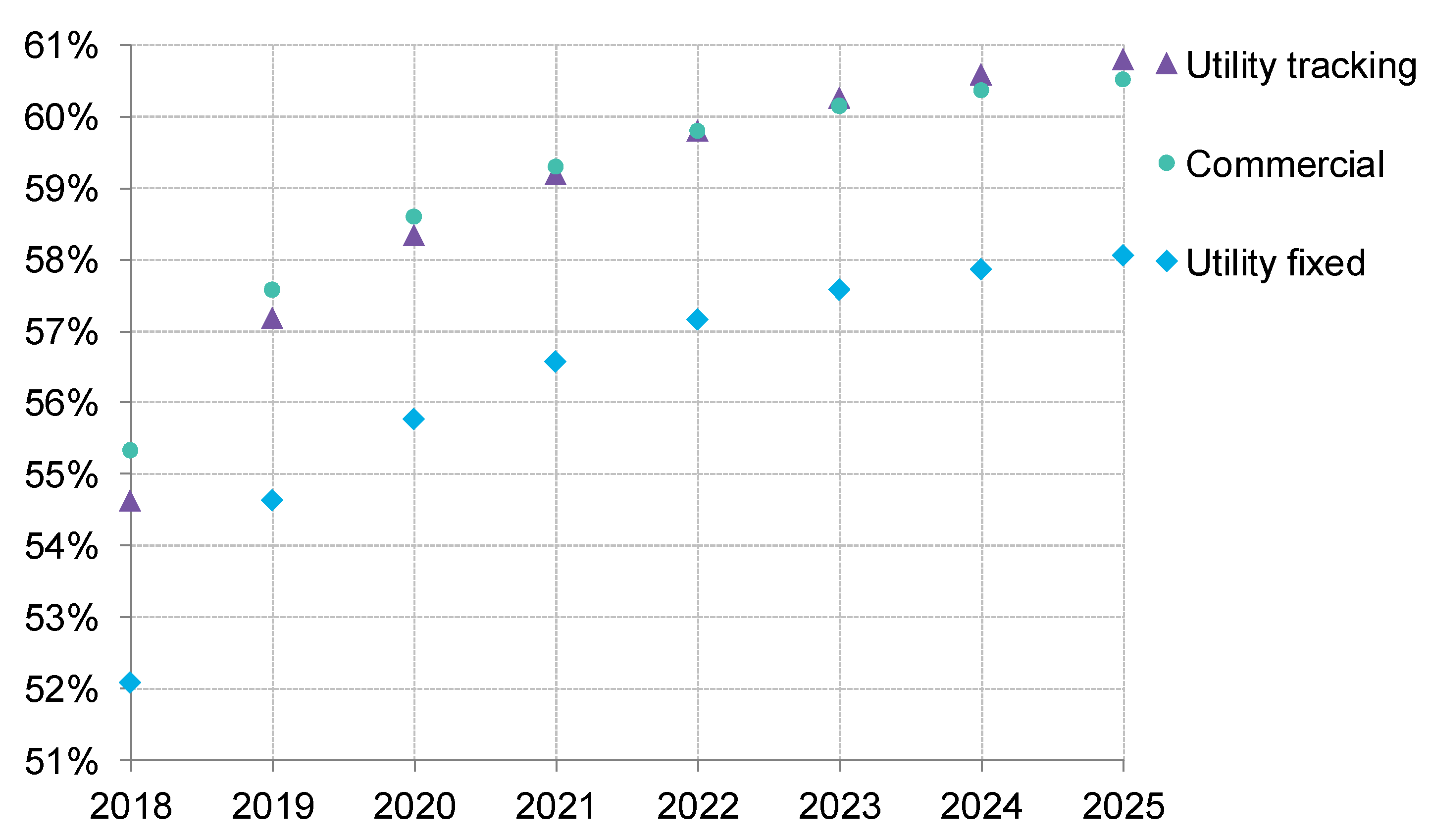
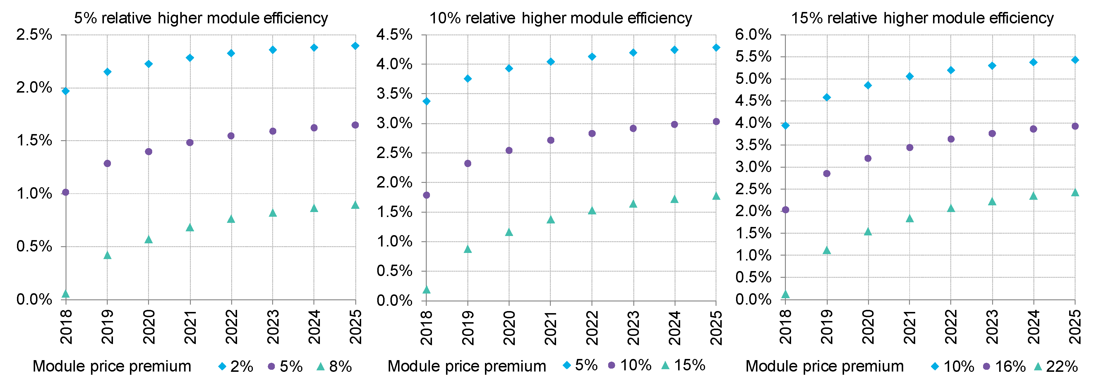
Module price reduction occurs faster than all other components in a PV system, resulting in a rising share of area-proportional and fixed non-module costs in the total system spending. As tracking is becoming a standard option for utility PV in sunny places [15], and the percentage of area-proportional and fixed non-module costs is similar for tracking utility and commercial PV, here we use the tracking utility to illustrate the evolving value of module efficiency, as shown in Figure 11. As time goes on, the value of module efficiency becomes greater, increasing the incentive to adopt high-efficiency technologies.
5. Bifacial Modules: Not a Simple Story about Higher Efficiency
By revising solar cells’ rear side electrical contact structure and replacing the opaque backsheet with glass, a PV module can convert light striking from the backside to electricity. This type of new products are referred as bifacial modules. A term ‘bifaciality’ describes how good the rear side efficiency is, compared with the front side, and is expressed as the ratio between the two:
The output from a bifacial module is expressed as the yield from both sides:
The bifacial yield gain compared with monofacial is the product of bifaciality and the ratio between input power from the rear side and that from the front side:
The second term in the above equation is referred to as the bifacial ratio, which is affected by many factors, including the reflectivity of the ground (or albedo), the angular distribution of light, orientation of the module, the height of the module, shading of the surrounding objects, etc. While some demonstration projects prove the bifacial gain can be higher than 20% [18,19], those achievements occurred with highly reflective ground and the projects are of small sales, so the gains are not considered representative. There is no standard bifacial ratio when measuring bifacial modules, although the National Renewable Energy Laboratory and Sandia National Laboratories suggested 130–140 W/m2 as the representative irradiation for the rear side while maintaining 1000 W/m2 for the front side [20]. Applying a 13.5% bifacial ratio and 75% bifaciality, a 10% bifacial gain is derived. However, in the real market, developers are only accepting a 5% bifacial gain assumption in price negotiation, considering there are still uncertainties about the new technologies without enough field operation data.
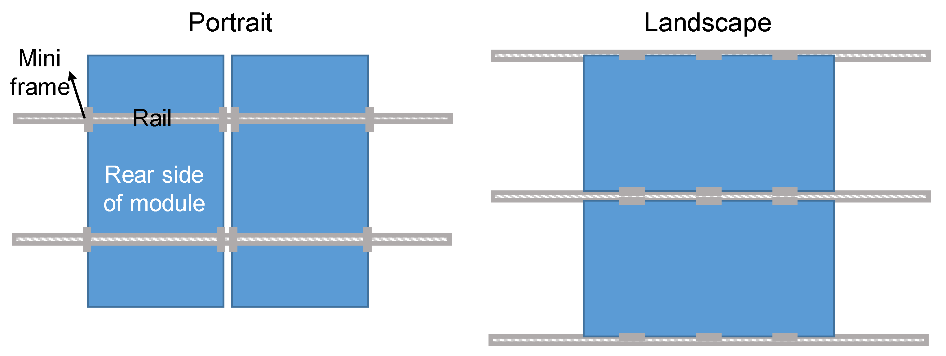
Although the bifacial gain is caused by more input power, rather than higher conversion efficiency, the effect is the same. According to the left-hand chart in Figure 11, bifacial modules that can be considered 5% relatively more efficient can ask for a price premium of up to 8% in utility PV projects in 2018. However, extra costs will be introduced at the system level in order to avoid shading to the rear side. Figure 12 shows the necessary changes for racking in a fixed-tilt scenario.
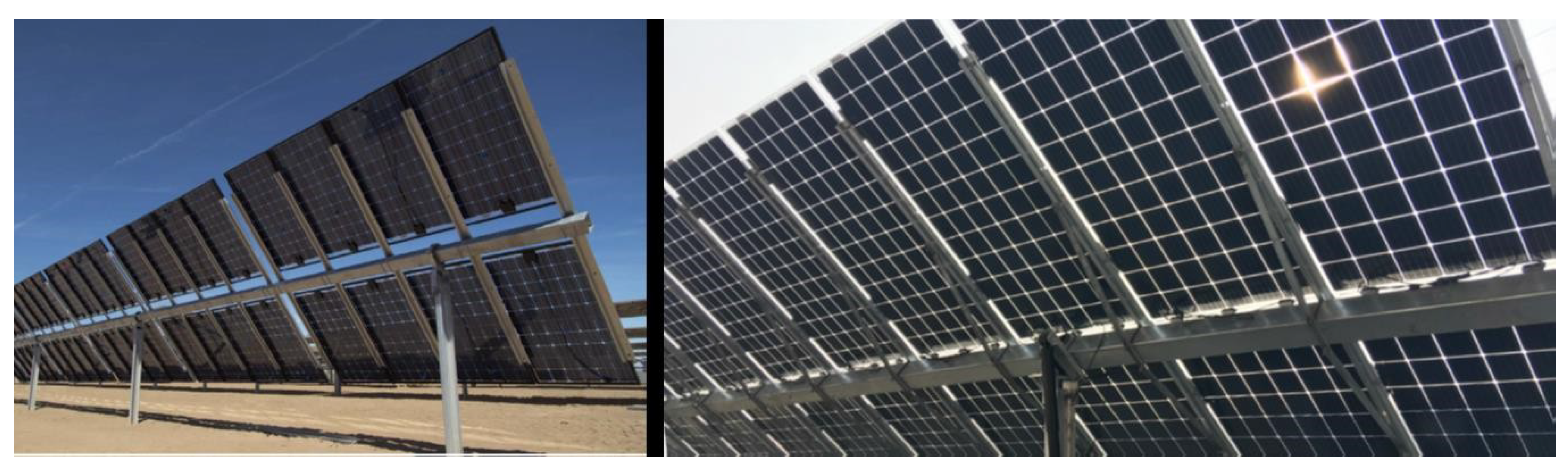
Figure 13 shows two trackers designed for bifacial modules. In both cases, the rails are positioned in the space between neighboring modules to avoid shading to the backside. In order to achieve the same mechanical stability, the metal consumption increases, resulting in an additional cost for trackers or fixed racking systems. Therefore, bifacial modules only receive a 3–4% price premium, with the power rating defined by the front-side yield. Even that value is sufficient to cover the extra cost. Therefore, we expect bifacial modules will see a rising market share, starting from 3GW global shipment, or a 3% share of total module shipment in 2018. BloombergNEF expects the global share to rise to 10% in 2020 and 40% in 2025 [21].
6. Discussion
The above analysis addresses the value of module efficiency for the dominant equipment type (modules composed of cells made of p-type crystalline silicon wafers) and major system configurations (fixed-tilt and one-axis tracking). We expand the discussion to other scenarios for niche market applications.
6.1. N-Type Crystalline Silicon Modules and Thin-Film Modules
2018 was the first year when the annual new PV build exceeded 100GW. Among all modules installed in 2018, 97% were of crystalline silicon types and only 3% were categorized as thin film modules, mainly supplied by First Solar (Tempe, AZ, USA) adopting cadmium telluride (CdTe) technologies and Solar Frontier (Tokyo, Japan) making copper indium selenium (CIS) products. While these thin-film modules have achieved efficiencies comparable to multicrystalline silicon products, their costs did not drop as rapidly as the c-Si peers. Considering the established advantages and sustainable approaches to even lower cost and higher efficiency for c-Si PV modules, it is unlikely for thin film to grow to a dominant share in the next 10 years.
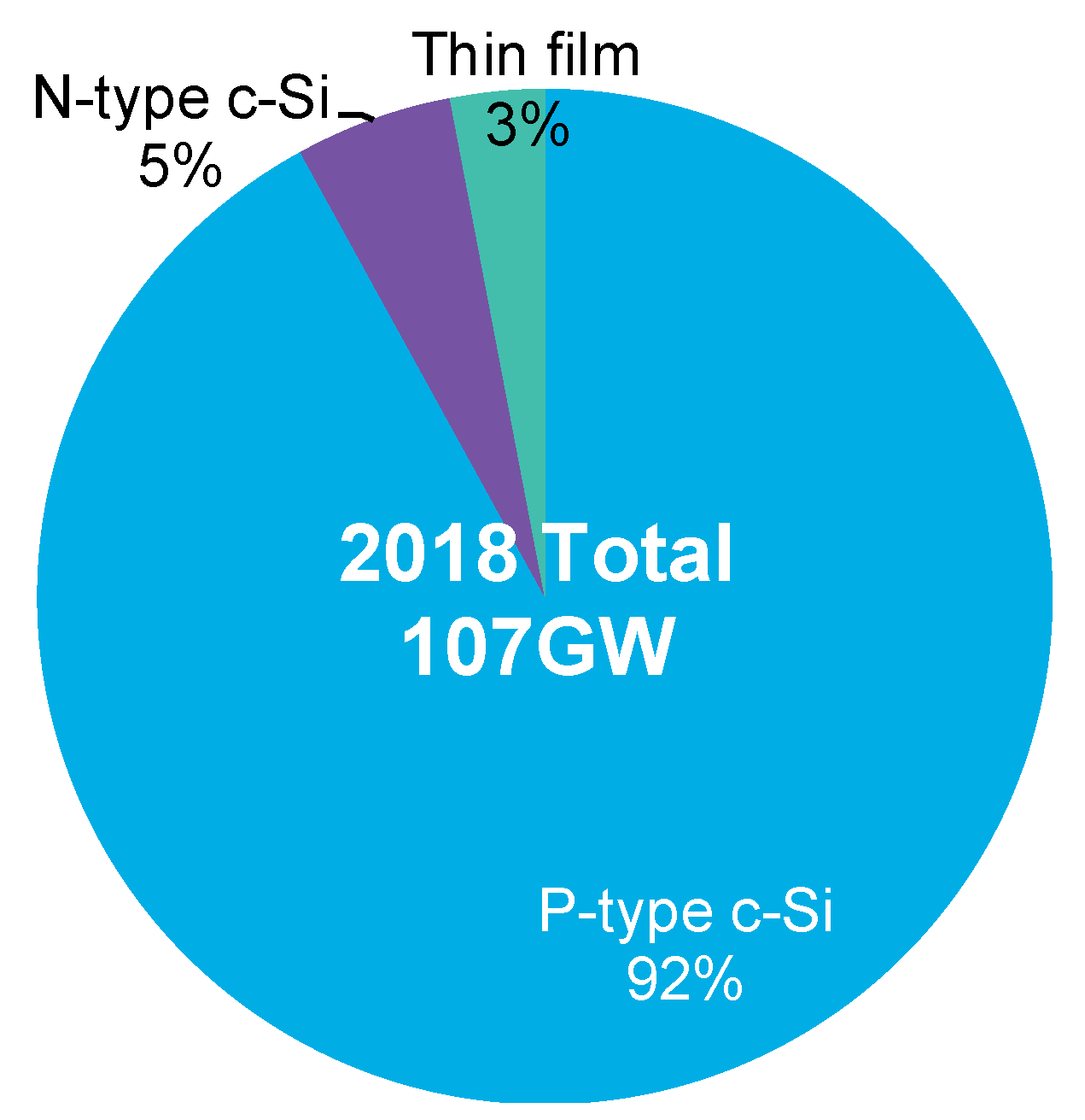
Looking into the general category of crystalline silicon PV modules, it can be further separated into more sub-groups depending on the definition. The most popular sub-grouping is multi- vs. monocrystalline silicon PV, based on the crystalline structure quality of wafers. Alternatively, based on the doping materials in wafers, c-Si can be divided into negatively doped (with boron) and positively doped (with phosphorous), or simplified referred in industry as n-type and p-type c-Si PV. N-type cells allow higher efficiencies, as the excited electrons in n-type wafers can travel a longer distance before they return to the useless bonded status. However, they are more expensive to make. From the perspective of optimal economics at the system level, the industry showed more preference towards p-type c-Si PV (Figure 14).
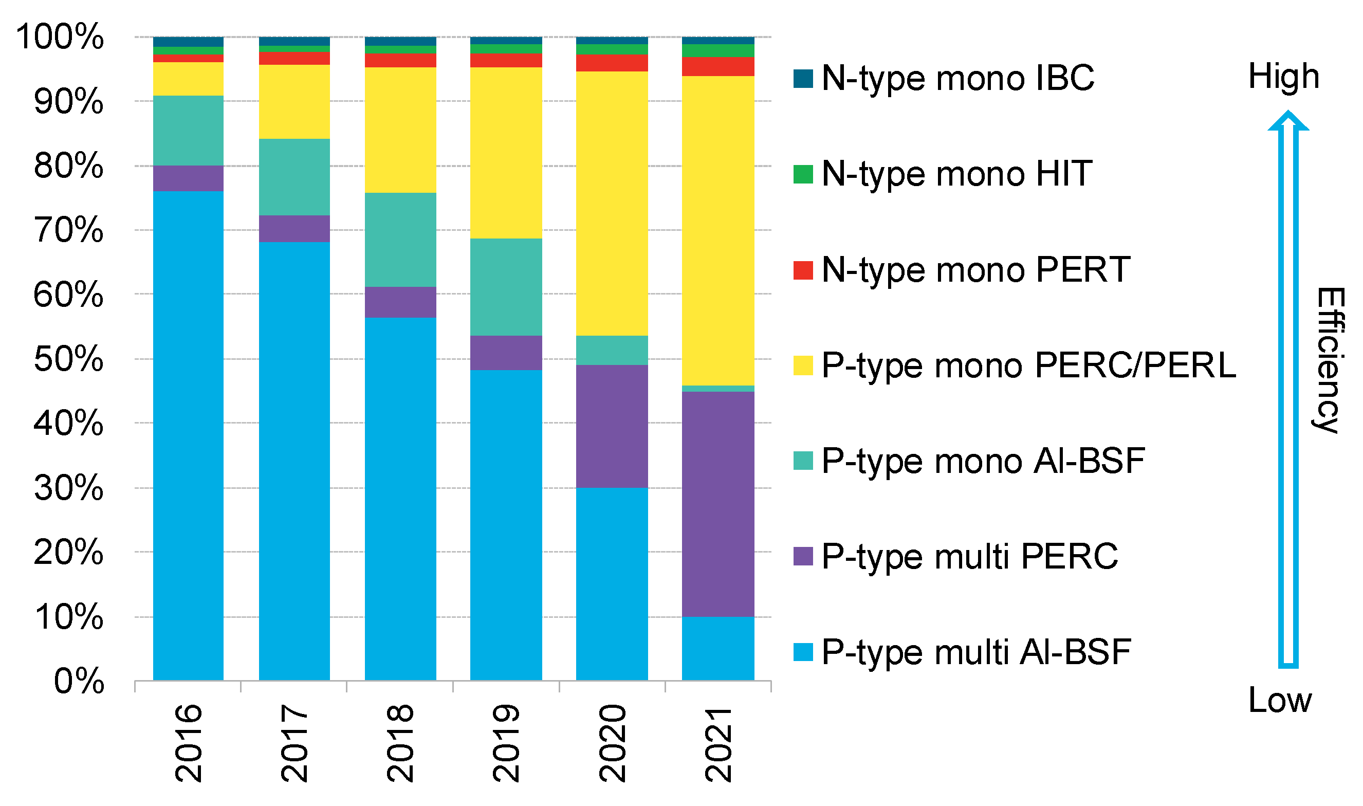
When cell structure is involved in categorizing PV modules, there are more options (Figure 15). Note that not every combination of different metrics has commercial applications because some combinations have poor economic value. For instance, there are no p-type IBC or HIT in the market, although theoretically such products can be made. Their absence from the market is because realizing these special cell structures necessitates higher production costs, but the p-type wafers cannot allow the advanced cell structures to fully display their capabilities of boosting efficiency and therefore do not justify the commercial production of such cells or modules. BloombergNEF observed a rising market share of PV modules with higher efficiencies, and expects the same trend to continue. However, p-type crystalline silicon PV modules are still likely to dominate in the near future, although monocrystalline silicon will win over its multi-peers soon.
When comparing the economics of different types of modules, more metrics should be brought into consideration besides module efficiency. Two important ones are temperature coefficient and degradation rate. While the module efficiency is measured under standard testing conditions, the actual operation environment varies constantly, and modules with the same area and efficiency (and thus the same nameplate capacity) but different materials or cell structures could generate different yields. One reason is that their operating efficiency could respond to the temperature change with various sensitivities, which is measured with a temperature coefficient with a unit of %/°C. For instance, cells made on p-type wafers (multi and mono) have TC around −0.43%/°C. N-type cells’ TC is around −0.30%/°C. Assuming the average cell temperature in the field is 20 °C higher than the standard testing condition, n-type IBC PV modules have 2.6% more yield than p-type mono PERC products for the same nameplate power rating, and this gap cannot be captured by efficiency.
Another important metric that affects actual yield is degradation rate, which measures how fast module efficiency declines over time. For example, Jinko Solar’s mono PERC modules have a warranty for 3% degradation in the first year and 0.7% linear annual degradation in the following 24 years, suggesting the warranted module efficiency at the end of the 25th year will be 80.2% that of the original nameplate efficiency. First Solar’s CdTe thin film module power warranty includes a starting point of 2% degradation for the first year and a 0.5% annual drop afterwards until the 25th year, indicating that the warranted module efficiency at the end of the 25th year will be 86% of the original nameplate efficiency. In a simplified assumption, where the annual illumination is the same over the 25-year period, First Solar’s modules could generate 4% more electricity than Jinko Solar’s modules of the same nameplate capacity.
Note that the purpose of deploying the discussion above is to illustrate the limitation of relying solely on module efficiency when evaluating actual performance and LCOE, rather than to set up a complete model to compare different types of modules.
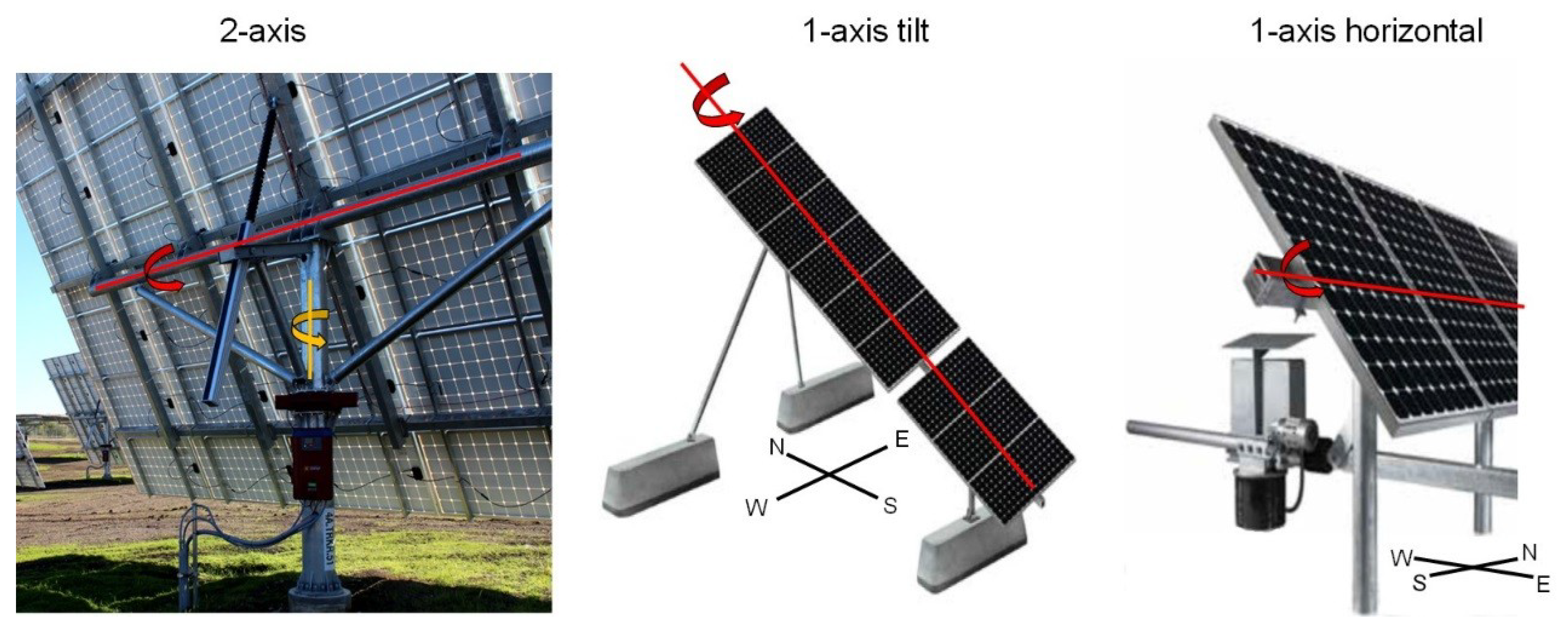
6.2. Different Tracking Options
As shown in Figure 16, there are three types of trackers available for PV modules. When mounted on a two-axis tracker, a PV module can receive direct light perpendicularly. Alternatively, a one-axis tracker can track the more dominant sun movement along the east–west direction, while sacrificing the accuracy on the north–south dimension and saving on equipment. Depending on the relative angle between the rotation pivot and the ground, one-axis trackers have two options: horizontal and tilt (Figure 16).
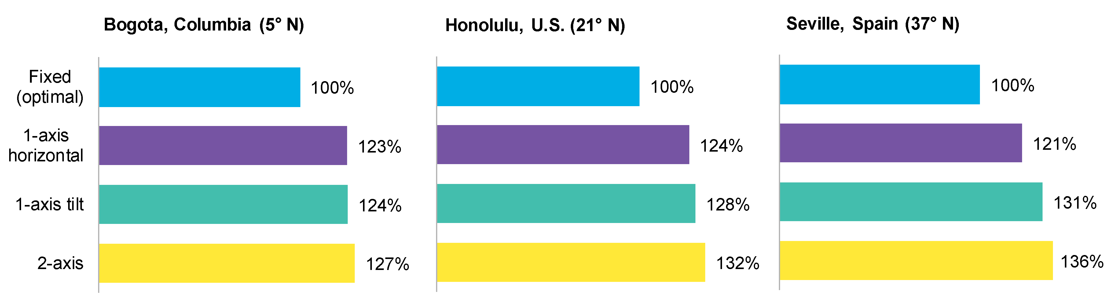
Although all three trackers have been commercialized at some point, one-axis horizontal is the only type that is still being applied in utility-scale PV projects. While the input power gain compared with the fixed tilt by different trackers varies depending on the latitude (Figure 17), the general conclusion holds that the additional yield when choosing one-axis tilt tracker and two-axis trackers over one-axis horizontal trackers cannot justify the much greater capital costs and long-term maintenance fees [15].
Therefore, we consider it less valuable to conduct a detailed analysis of the impact of module efficiency on system LCOE in configurations adopting one-axis tilt trackers or two-axis trackers. However, it is understandable that in those systems, area-related non-module costs account for a higher percentage of the total system spending, and a certain module efficiency rise can impose a stronger leverage in lowering system cost and therefore LCOE. In fact, most of the two-axis tracker shipments in history were for systems adopting concentrator PV (CPV) modules composed of multi-junction solar cells with module efficiencies up to 30%, although the module efficiency testing condition for CPV modules is different from that for flat-plate PV modules [22].
7. Conclusions
While the record efficiencies tested in research labs demonstrated the achievable performance of PV modules, they do not suggest immediate adoption of the corresponding process technologies in the industry, which could result in significant additional costs. This paper aims to help academics, representatives of industry, and policy makers to develop a better understanding of the value of module efficiency by deploying quantitative analyses at the PV system level, for the current market and for the future. The readers of this paper will be able to adopt benchmark values and methodology to derive an estimate of the market recognition for any new product.
Author Contributions
Conceptualization, X.W. and A.B.; Methodology, X.W.; Software, X.W.; Validation, X.W. and A.B.; Formal Analysis, X.W.; Resources, X.W. and A.B.; Writing–Original Draft Preparation, X.W.; Writing–Review & Editing, X.W. and A.B.
Funding
This research received no external funding.
Conflicts of Interest
The authors declare no conflict of interest.
Appendix A

Table A1.
Symbol list for equations in this paper.
| Symbol | Metric | Unit |
|---|---|---|
| LCOE | Levelized cost of electricity | $/kWh |
| TLCC | Total life-cycle cost | $ |
| Cn | Cost for year n | $ |
| Qn | Energy output for year n | kWh |
| N | Analysis period | Year |
| d | Discount rate | % |
| β | Bifaciality | % |
| ηfront | Front side module efficiency | % |
| ηrear | Rear side module efficiency | % |
| Pout | Total output power from the module | kWh |
| Pinfront | Input power from module front side | kWh |
| Pinrear | Input power from module rear side | kWh |
| Gain | Output from module rear side relative to output from front side | % |
References
- Swarbreck, J.; Chase, J.; Radoia, P.; Bromley, H.; Wang, X.; Hayim, L. 2018 Long-Term PV Market Outlook; BloombergNEF Research: New York, NY, USA, 2018. [Google Scholar]
- Henbest, S.; Chase, J.; Grace, A.; Goldie-Scot, L.; Rooze, J.; Chatterton, R.; Giannakopoulou, E.; Lu, S.; Harries, T.; Turner, A.; Kimmel, M. New Energy Outlook 2018; BloombergNEF Research: New York, NY, USA, 2018. [Google Scholar]
- Hayim, L.; Chase, J. Socket Parity Is Here, But Solar Adoption Needs More; BloombergNEF Research: New York, NY, USA, 2017. [Google Scholar]
- D’Adamo, I. The Profitability of Residential Photovoltaic Systems. A New Scheme of Subsidies Based on the Price of CO2 in a Developed PV Market. Soc. Sci. 2018, 7, 148. [Google Scholar] [CrossRef]
- Wang, X.; Chase, J. Solar-Storage Design Synergies Support Dispatchable PV; BloombergNEF Research: New York, NY, USA, 2018. [Google Scholar]
- Tavakkoli, M.; Pouresmaeil, E.; Godina, R.; Vechiu, I.; Catalão, J.P. Optimal Management of an Energy Storage Unit in a PV-Based Microgrid Integrating Uncertainty and Risk. Appl. Sci. 2019, 9, 169. [Google Scholar] [CrossRef]
- Radoia, P.; Bromley, H.; Wang, X.; Jiang, Y.; Swarbreck, J.; L’Ecluse, C. 3Q 2018 Global PV Market Outlook; BloombergNEF Research: New York, NY, USA, 2018. [Google Scholar]
- Wang, X.; Kurdgalashvili, L.; Byrne, J.; Barnett, A. The Value of Module Efficiency in Lowering the Levelized Cost of Energy of Photovoltaic Systems. Renew. Sustain. Energy Rev. 2011, 15, 4248–4254. [Google Scholar] [CrossRef]
- Short, W.; Packey, D.; Holt, T. A Manual for the Economic Evaluation of Energy Efficiency and Renewable Energy Technologies; NREL/TP-462-5173; National Renewable Energy Lab.: Golden, CO, USA, 1995.
- Wang, X.; Goldie-Scot, L.; Bromley, H.; Narayanan, T. 2018 SPI takeaway: Trend is Stronger than Policy; BloombergNEF Research: New York, NY, USA, 2018. [Google Scholar]
- Fu, R.; Feldman, D.; Margolis, R. U.S. Solar Photovoltaic System Cost Benchmark: Q1 2018; National Renewable Energy Laboratories report; National Renewable Energy Lab.: Golden, CO, USA, 2018.
- Wang, X.; Byrne, J.; Kurdgalashvili, L.; Barnett, A. High efficiency photovoltaics: On the way to becoming a major electricity source. WIREs Energy Environ. 2012, 1, 132–151. [Google Scholar] [CrossRef]
- Barnett, A.; Wang, X. High efficiency photovoltaics lead to low energy cost. In Green Energy Economies: The Search for Clean and Renewable Energy; Transaction Publishers: Piscataway, NJ, USA, 2014. [Google Scholar]
- Jiang, Y.; Wang, X. 2018 PV Manufacturing Overview: From Polysilicon to Module; BloombergNEF Research: New York, NY, USA, 2018. [Google Scholar]
- Wang, X. Tracking the Sun Has a Bright Future; BloombergNEF Research: New York, NY, USA, 2017. [Google Scholar]
- Yu, Z.; Carpenter, J.V.; Holman, Z. Techno-economic viability of silicon-based tandem photovoltaic modules in the United States. Nat. Energy 2018, 3, 747–753. [Google Scholar] [CrossRef]
- Peters, I.M.; Sofia, S.; Mailoa, J.; Buonassisi, T. Techno-economic analysis of tandem photovoltaic systems. RSC Adv. 2016, 6, 66911–66923. [Google Scholar] [CrossRef]
- PVG Solutions. World First Large Scale 1.25MW Bifacial PV Power Plant on Snowy Area in Japan; PVG Solutions: Miyazaki, Japan, 2016. [Google Scholar]
- Stein, J.S.; Burnham, L.; Lave, M. One Year Performance Results for the Prism Solar Installation at the New Mexico Regional Test Center; Sandia National Laboratories report; Sandia National Laboratories: Albuquerque, NM, USA; Livermore, CA, USA, 2017.
- Deline, C.; MacAlpine, S.; Marion, B. Evaluation and Field Assessment of Bifacial Photovoltaic Module Power Rating Methodologies; National Renewable Energy Laboratories report; National Renewable Energy Lab.: Golden, CO, USA, 2016.
- Wang, X. Bifacial Solar Modules See Both Sides; BloombergNEF Research: New York, NY, USA, 2018. [Google Scholar]
- Wang, X. Focus on concentrator PV Technology; BloombergNEF Research: New York, NY, USA, 2012. [Google Scholar]
Figure 1.
Learning rate of crystalline silicon modules.

Figure 2.
Global electricity generation mix. Note: NEO is short for new energy outlook, which is an annual publication by BloombergNEF.
Figure 2.
Global electricity generation mix. Note: NEO is short for new energy outlook, which is an annual publication by BloombergNEF.

Figure 3.
Commercial PV socket parity in 2017 and 2025 with 75% on-site consumption. Note: Generation-based subsidies (in terms of $/kWh) are excluded in the calculation.
Figure 3.
Commercial PV socket parity in 2017 and 2025 with 75% on-site consumption. Note: Generation-based subsidies (in terms of $/kWh) are excluded in the calculation.

Figure 4.
Cost structure of a utility-scale PV project in 2018. Note: Module efficiency for this example project is 17.7%.
Figure 4.
Cost structure of a utility-scale PV project in 2018. Note: Module efficiency for this example project is 17.7%.

Figure 5.
Impact of module efficiency on PV system cost and module price premium. Note: In the left-hand chart, the relative change in terms of percentage refers to the non-module unit cost of the benchmark case as shown in Figure 4. In the right-hand chart, the reference is the module unit cost of the benchmark case in Figure 4.
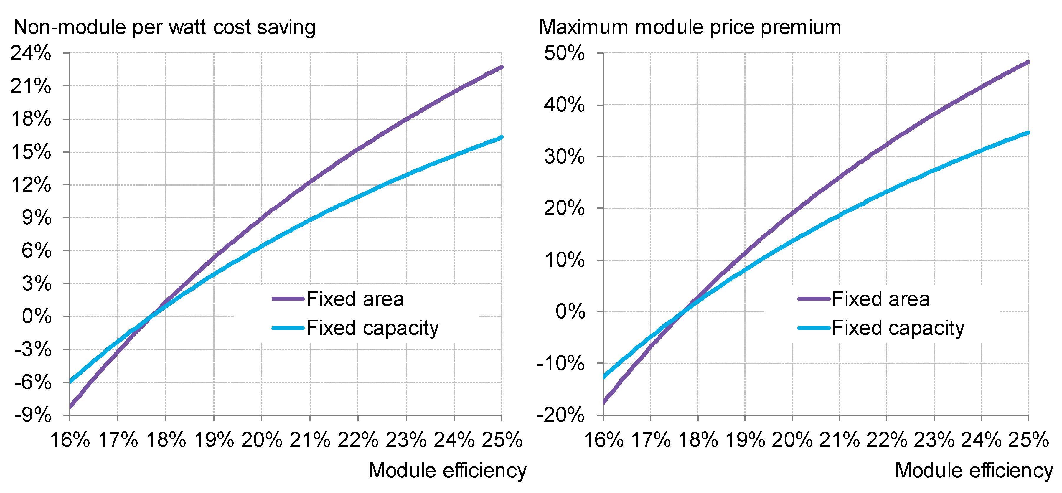
Figure 6.
2018 benchmark of PV system capex ($/WDC). Source: BloombergNEF Note: The values presented in the right-hand chart are estimated from BloombergNEF benchmark costs. Module efficiency is 17.7% for the benchmark projects.
Figure 6.
2018 benchmark of PV system capex ($/WDC). Source: BloombergNEF Note: The values presented in the right-hand chart are estimated from BloombergNEF benchmark costs. Module efficiency is 17.7% for the benchmark projects.
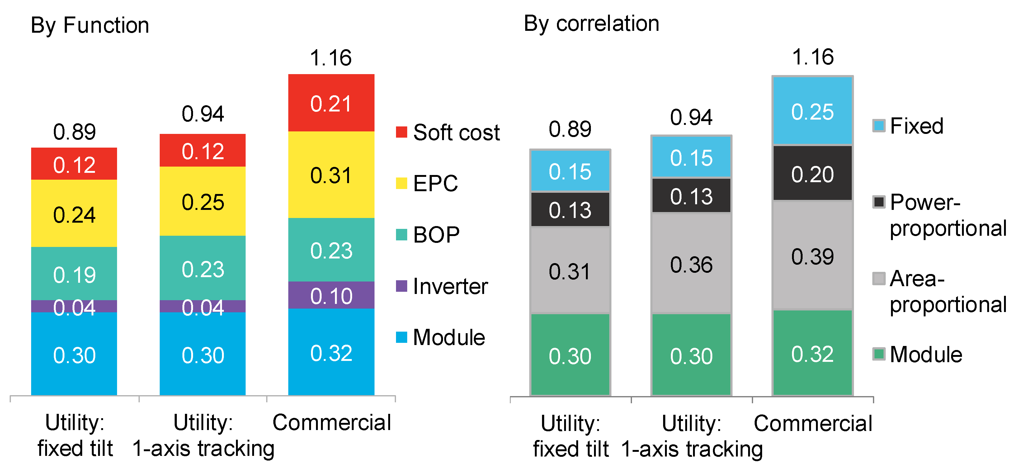
Figure 7.
Sensitivity of PV LCOE to module price and efficiency for (a) utility applications and (b) commercial applications. Note: The analysis is for cases without restriction on power capacity. ‘Tracking’ here assumes that one-axis horizontal trackers are adopted.
Figure 7.
Sensitivity of PV LCOE to module price and efficiency for (a) utility applications and (b) commercial applications. Note: The analysis is for cases without restriction on power capacity. ‘Tracking’ here assumes that one-axis horizontal trackers are adopted.

Figure 8.
Residential PV system costs in different markets.

Figure 9.
Forecast of best-case integrated production cost for c-Si modules. Source: BloombergNEF Note: Integrated production refers to the operation model of sourcing polysilicon from the spot market and implementing the rest of the process using an in-house facility.
Figure 9.
Forecast of best-case integrated production cost for c-Si modules. Source: BloombergNEF Note: Integrated production refers to the operation model of sourcing polysilicon from the spot market and implementing the rest of the process using an in-house facility.

Figure 10.
Estimated percentage of area-proportional and fixed non-module costs in PV capex.

Figure 11.
PV LCOE reduction vs. module efficiency and module price, 2018–2025. Note: The module efficiency compared with the benchmark in a specific year. For instance, 5% relative higher module efficiency in 2018 points to a module efficiency at 17.7%*1.05, or 18.6%. 15% relative higher module efficiency in 2025 points to a module efficiency at (17.7%*1.025^7)*1.15, or 24.2%. In this paper, we focus on efficiencies that are likely to be adopted by the market in the near future. However, much greater efficiencies based on tandem solar cells have been realized in lab research [16,17].

Figure 12.
Two installation profiles of modules with mini frames.

Figure 13.
One-axis trackers designed for bifacial modules.

Figure 14.
2018 global PV module shipment by product type.

Figure 15.
Market share of different c-Si PV modules. Note: IBC is short for interdigitated back contact. HIT: heterojunction with intrinsic thin layer. PERC: passivated emitter and rear cell. PERL: passivated emitter, rear locally-diffused. PERT: passivated emitter, rear totally-diffused. Al-BSF: aluminum back surface field. Source: BloombergNEF.

Figure 16.
Three types of PV trackers defined by tracking dimension.

Figure 17.
2018 annual irradiation collected by a PV module in different mounting scenarios.

© 2019 by the authors. Licensee MDPI, Basel, Switzerland. This article is an open access article distributed under the terms and conditions of the Creative Commons Attribution (CC BY) license (http://creativecommons.org/licenses/by/4.0/).
Share and Cite
MDPI and ACS Style
Wang, X.; Barnett, A. The Evolving Value of Photovoltaic Module Efficiency. Appl. Sci. 2019, 9, 1227. https://doi.org/10.3390/app9061227
AMA Style
Wang X, Barnett A. The Evolving Value of Photovoltaic Module Efficiency. Applied Sciences. 2019; 9(6):1227. https://doi.org/10.3390/app9061227
Chicago/Turabian StyleWang, Xiaoting, and Allen Barnett. 2019. "The Evolving Value of Photovoltaic Module Efficiency" Applied Sciences 9, no. 6: 1227. https://doi.org/10.3390/app9061227
Note that from the first issue of 2016, this journal uses article numbers instead of page numbers. See further details here.