A New Method of Simultaneous Localization and Mapping for Mobile Robots Using Acoustic Landmarks

Abstract

The simultaneous localization and mapping (SLAM) problem for mobile robots has always been a hotspot in the field of robotics. Simultaneous localization and mapping for robots using visual sensors and laser radar is easily affected by the field of view and ground conditions. According to the problems of traditional sensors applied in SLAM, this paper presents a novel method to perform SLAM using acoustic signals. This method enables robots equipped with sound sources, moving within a working environment and interacting with microphones of interest, to locate itself and map the objects simultaneously. In our case, a method of microphone localization based on a sound source array is proposed, and it was applied as a pre-processing step to the SLAM procedure. A microphone capable of receiving sound signals can be directly used as a feature landmark of a robot observation model without feature extraction. Meanwhile, to eliminate the random error caused by hardware equipment, a sound settled in the middle of two microphones was applied as a calibration sound source to determine the value of the random error. Simulations and realistic experimental results demonstrate the feasibility and effectiveness of the proposed method.

1. Introduction

With the development of science and technology, the robot market has grown quite large for a myriad of applications. The realization of autonomous navigation for robots is an important step in solving the difficult problems of various complicated working environments. Simultaneous localization and mapping (SLAM) [1,2,3,4] of mobile robots is a fundamental and important problem rooting from the related research. In the SLAM problem, the robot needs to perceive its own movement behavior, pose, and information of the current environment through sensors when it is in a known or unknown environment. Visual and optical sensors are classically used as external sensors in solving problems of SLAM [5,6,7,8,9]. In Reference [10], the technology of the robot environment map-building based on laser radar scanner was studied. However, the beam of the laser radar was extremely narrow, making it difficult to search for targets in space. Its accuracy was also greatly affected by the ground conditions. In Reference [11], a moving camera was applied to adopt environmental information. Then, a visualized SLAM solution was implemented through combining the extended Kalman filtering technology with extracted image features. It needs to be pointed out that visual sensors can only perceive information within the robot’s limited field of vision and rely heavily on light. Compared with the above external sensors, sound has the advantages of propagation omnidirectionality, diffraction susceptibility, high-time resolution, and non-limited visibility. In contrast to the classical context of SLAM, this paper presents an algorithm to perform SLAM using acoustic signals. Acoustic SLAM has the potential for wide application in areas including autonomous robots, hearing aids, smart cars, and virtual reality devices [12,13].

An audition system is a very important feature for an intelligent robot [14,15,16]. In the auditory field, there are several research issues such as sound source localization, localization of moving microphone arrays, speech separation and enhancement, etc. [17,18,19,20,21,22]. Time delay of arrival (TDOA) between sound sources and corresponding microphones was always used in the studies mentioned above [23]. The localization of microphones may help to solve a number of problems for mobile robots. In this paper, acoustic SLAM typically applied microphone localization as a pre-processing step to the extended Kalman filter (EKF) procedure. The distances between the sound sources and detected microphones were calculated according to the TDOA obtained, and then they were used as direct measurement information for microphone localization. The time delay estimation method has a small number of calculations and strong real-time performance. Commonly used time delay estimation algorithms include generalized cross-correlation (GCC) [24], cross-power spectral phase (CSP) [25], adaptive filtering [26], etc. Among them, the GCC method exhibits superior performance in suppressing noise and reverberation. Sekmen et al. [27] proposed a natural way of human–computer interaction in which people as passive users did not need to interact with the robot through keyboards, mice, etc. The method assumed that the sound source was located in front of the robot, and the cross-correlation method could be used to estimate the time difference of the sound, and then the far-field sound source was located by the far-field approximation geometric method. Hu et al. [28,29] used the generalized cross-correlation method based on feature structure to estimate the time difference of sound of multiple sound sources. This paper estimates time delay between sound source and microphone by use of the GCC method.

At present, solutions to the SLAM problem are roughly divided into two categories: methods based on probability estimation and methods based on non-probabilistic estimation. The basis of the probabilistic estimation method is mainly Bayesian theory estimation, which is divided into two major filtering algorithms: Kalman filter and particle filter. A number of studies have been conducted on the basis of them, and several classical algorithms have been proposed, such as the EKF [30], the unscented Kalman filter (UKF) [31,32], the particle filter and the Rao–Blackwellization algorithm, the particle filter combined with the Rao–Blackwellization algorithm to form RBPF [33,34,35,36], etc. Reference [37] has made a detailed comparison of the above algorithms. Among them, EKF-based SLAM is simple and feasible when dealing with non-linear systems, and it is still widely used not only in land, aviation, and underwater fields, but also in various forms of robotics, such as unmanned aerial vehicles (UAVs) [38], automated guided vehicles (AGVs) [39], and remotely operated vehicles (ROVs) [40].

In this paper, we propose a novel approach to map the positions of microphones passively and to simultaneously localize a moving robot in realistic acoustic environments. The microphone localization process based on sound source array was conducted and then a method of EKF-SLAM for mobile robots based on microphone landmark observation is proposed. To avoid the estimation error of the time delay of sound arrival caused by environmental noise, reverberation [41], and hardware equipment, a method of using calibration to eliminate TDOA estimating errors is presented.

In our case, the robot itself carries three sound source units distributed in an equilateral triangle and a reference microphone. The relative distance between the reference microphone and the three sound sources was known. The reference microphone was placed within a range that ensured that the three sound signals could be received clearly. In the same plane as the sound sources, a certain number of microphones were randomly distributed; the microphone which received the three sound signals was defined as a microphone to be positioned (MTP). The reference frames are illustrated in Figure 1.

Therefore, the novel features of the approach proposed in this paper are (1) the joint estimation of the unknown robot path and the positions of multiple microphones based on the (2) sound source array installed on the robot, and (3) a microphone capable of receiving sound signals which can be directly used as a feature landmark of the robot observation model without feature extraction. Performance results for controlled and realistic room acoustics are presented to analyze the theoretical and practical behavior of the method. Specifically, it is shown that this approach outperforms other methods for SLAM due to its lower complexity and lack of feature extraction, and SLAM research using acoustic sensors has the potential for wide application.

The paper is structured as follows: Section 2 describes the strategy of the microphone localization method based on sound source array. Section 3 derives the proposed algorithm involving the microphone localization combined with EKF-SLAM. Section 4 presents the simulation and experimental setup and results. Conclusions are drawn in Section 5.

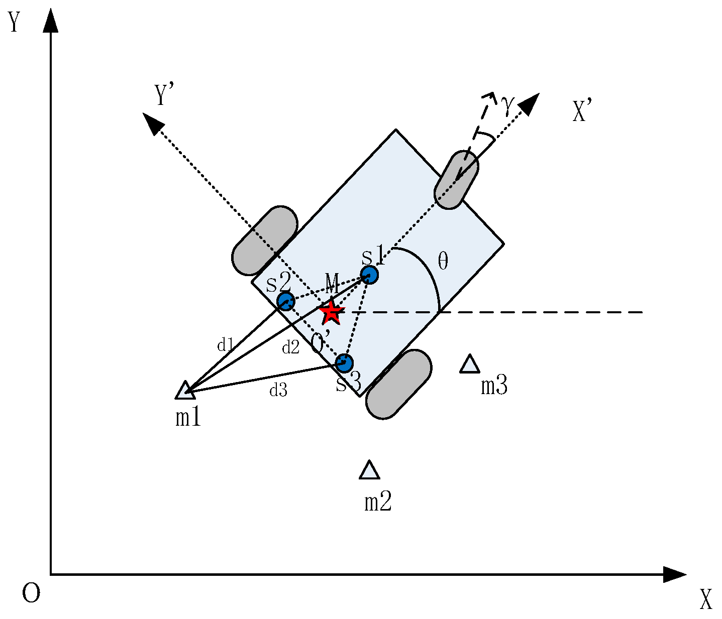
2. Localization of Microphones Based on Sound Source Array

2.1. Time Delay of Arrival (TDOA) Estimation

The GCC algorithm is currently the most widely used time estimation method. Aiming at the existence of a large amount of noise and reverberation in the actual environment, and thus causing the maximum peak value of the cross-correlation function to be inconspicuous or to have multiple peaks, GCC is better than the basic cross-correlation algorithm for its ability to suppress noise and reverberation in terms of peak detection difficulty. It is assumed here that the sound signal model received by the microphone is an ideal model; that means only ambient noise is considered. The ambient noise is approximately replaced by white Gaussian noise [42,43]. It is also assumed that there is no correlation between noise and noise, and noise and sound source. The mathematical model of the signal received by the microphone is shown as

$$x_i\left(t\right)={\alpha }_{i}s\left(t-{\tau }_i\right)+n_i\left(t\right)$$

(1)

where considering the sound signal $s\left(t\right)$, the signal received by the i-th microphone $x_i\left(t\right)$, ${\alpha }_i$, ${\tau }_i$, and $n_i\left(t\right)$ represent the amplitude attenuation coefficient, time delay, and ambient noise of the sound signal reaching the i-th microphone, respectively. The cross-correlation function of sound signals reached to the i-th and j-th microphone is shown as

$$R_{x_i{x}_j}\left(\tau \right)=E\left[x_i\left(t\right)x_j\left(t-\tau \right)\right]$$

(2)

Since noise and noise, and noise and sound source are not related to each other, Equation (3) can be derived from Equations (1) and (2):

$$R_{x_i{x}_j}\left(\tau \right)={\alpha }_i{\alpha }_j{R}_{ss}\left(\tau -{\tau }_{ij}\right)$$

(3)

where $R_{ss}\left(\tau \right)$ is the autocorrelation function of $s\left(t\right)$, ${\tau }_{ij}$ is the relative time delay in which the i-th and j-th microphones receive the sound signal. According to the nature of the autocorrelation function, it is known that $R_{x_i{x}_j}\left(\tau \right)$ reaches the maximum value when $\tau -{\tau }_{ij}=0$. Then the time delay estimate ${\tau }_{ij}$ can be calculated according to the cross-correlation function of the signals received by the two microphones and the point where the maximum value is located. Equation (4) is obtained by Fourier transform [44,45] of Equation (3)

$${\phi }_{x_i{x}_j}\left(\omega \right)={\alpha }_i{\alpha }_j{\phi }_{ss}\left(\omega \right)e^{-j\omega {\tau }_{ij}}+{\phi }_{n_i{n}_j}\left(\omega \right)$$

(4)

where ${\phi }_{ss}\left(\omega \right)$, ${\phi }_{x_i{x}_j}\left(\omega \right)$, and ${\phi }_{n_i{n}_j}\left(\omega \right)$ represent the corresponding power spectrum of $R_{ss}\left(\tau \right)$, $R_{x_i{x}_j}\left(\tau \right)$, and $R_{n_i{n}_j}\left(\tau \right)$, respectively. $R_{n_i{n}_j}\left(\tau \right)$ is the cross-correlation function of $n_i\left(t\right)$ and $n_j\left(t\right)$. Furthermore, by weighting Equation (4) and then performing the inverse transform, the generalized cross-correlation function can be obtained, as is shown

$$R_{ij}\left(\tau \right)=\underset{-\infty }{\overset{\infty }{{\displaystyle \int }}}{\phi }_{x_i{x}_j}\left(\omega \right){\theta }_{ij}\left(\omega \right)e^{j\omega \tau }d\omega$$

(5)

where ${\theta }_{ij}\left(\omega \right)$ is a generalized weighting function [46]. There are weighted functions such as Roth, SCOT (smooth coherent transformation), PHAT (phase transformation) [47,48,49], etc. As the PHAT weighting function has less volatility in the case of constantly changing signal-to-noise ratios, and the anti-noise performance is also better, the PHAT weighting function was selected for analysis in this paper. As shown in Figure 2, there was a part of a sound signal waveform received by two microphones (m0, m1). The frequency of the sound wave was 2 kHz, and the sampling frequency was 16 kHz.

Analyzing Figure 2, the time difference of arrival between m0 and m1 was approximately 0.008 s. In this paper, the GCC method was used to estimate the time difference of sound. As shown in Figure 3, according the values determined for the peak of the cross-correlation function, the TDOA can be estimated.

In Figure 3, the time corresponding to the position of the waveform peak was 0.01 s. This proves that the TDOA was well estimated using the GCC method.

2.2. Localization of Microphones

The implementation process of the microphone localization method based on sound source array was as follows. Given the position of the robot in the global coordinates, the position of the three sound sources and the reference microphone in the global coordinates could then be calculated. By obtaining TDOA, the distances between the microphone to be positioned (MTP) and the three sound sources were obtained through further calculation. Define $\Delta T_{ij}(i=1,2\dots N;j=1,2,3)$ as the time difference of receiving the j-th sound signal between the reference microphone and the i-th MTP, where N is the number of the MTP. Define the speed of sound propagation in the air as C, which is multiplied by the TDOA to obtain the difference value $\Delta L_{ij}$ about the distance from the j-th sound source to the reference microphone and to the i-th MTP.

$$\Delta L_{ij}=\Delta T_{ij}·C$$

(6)

$L_j\left(j=1,2,3\right)$ is defined as the distance from the reference microphone to the j-th sound source. Based on Equation (6) and $L_j\left(j=1,2,3\right)$, the distance between the i-th MTP and the j-th sound source can be calculated as follows

$$d_{ij}=L_j+\Delta L_{ij}=L_j+\Delta T_{ij}·C$$

(7)

Define $(x,y)$ as the position of the i-th MTP, and $\left(x_j,y_j\right)\left(j=1,2,3\right)$ as the position of the three sound sources in the global coordinate system. According to the geometric relationship, the position of the i-th MTP in the environment is obtained by solving the intersections of three circles with three sound source positions as centers and the distance from the microphone to the corresponding sound source as radius.

$$\{\begin{array}{l}{(x-x_1)}^2+{(y-y_1)}^2={d_{i1}}^2\\ {(x-x_2)}^2+{(y-y_2)}^2={d_{i2}}^2\\ {(x-x_3)}^2+{(y-y_3)}^2={d_{i3}}^2\end{array}$$

(8)

Here, $d_{i1}$, $d_{i2}$, and $d_{i3}$ represent the distance from the i-th MTP to the three sound sources, respectively. A block diagram overview of the microphone localization processing chain is provided in Figure 4.

3. Acoustic SLAM Based on Microphone Landmarks

The procedure of SLAM is to recognize a set of feature landmarks and localize the sensor odometer with respect to the landmark set. A sound source array carried by a robot was used in this paper to perform the localization of the robot and feature landmarks (microphones). According to Section 2, a microphone capable of receiving sound signals can be directly used as a feature landmark of a robot observation model without feature extraction. The distances were considered as the observation measurements and this became a standard range-only SLAM problem. The EKF-SLAM algorithm was adopted. It generally decreases the uncertainty of the system and the amount of calculations. During the SLAM process, the robot continuously acquires the landmark information while moving; the existing landmarks are used to correct the robot pose, and the new landmarks are used to incrementally construct the map of the surroundings.

3.1. EKF-SLAM Algorithm

Smith, Self, and Cheeseman [50] first proposed the SLAM algorithm, and used an extended Kalman filter to perform simultaneous estimations of the position of a robot and the landmarks observed. Assuming that the high-dimensional state vector $\mathrm{X}$ is the SLAM system state, which is specified as the robot’s pose (position and heading) and location of stationary landmarks observed in the environment

$$X={\left[X_r,X_1,X_2,\dots X_M\right]}^T$$

(9)

where ${\mathrm{X}}_{\mathrm{r}}={\left[x_r,y_r,{\theta }_r\right]}^T$ $X_r={\left[x_r,y_r,{\theta }_r\right]}^T$ represents the robot’s pose, among which $\left(x_r,y_r\right)$ are the coordinates of the robot in the global coordinate system, and ${\theta }_r$ represents the heading of the robot body, namely, the angle between the robot body and the x-axis of the global coordinate system. ${\mathrm{X}}_{\mathrm{i}}={\left[x_i,y_i\right]}^T,\left(i=1,2,\dots M\right)$ $X_i={\left[x_i,y_i\right]}^T,\left(i=1,2,\dots M\right)$ are the coordinates of the landmarks in the environment. The covariance matrix of the system is shown in Equation (10).

$$P=\left[\begin{array}{cccc}{P}_{rr}& P_{r1}& \dots & P_{rM}\\ P_{1r}& P_{11}& \dots & P_{1M}\\ \dots & \dots & \ddots & \dots \\ P_{Mr}& P_{M1}& \dots & P_{MM}\end{array}\right]$$

(10)

where ${\mathrm{P}}_{\mathrm{r}\mathrm{r}}$ indicates the covariance of the robot’s pose, ${\mathrm{P}}_{ij}\left(i=1,2,\dots ,M;j=1,2,\dots ,M\right)$ indicates the covariance of the landmark location, ${\mathrm{P}}_{ri}\left(i=1,2,\dots ,M\right)$ represents the covariance between the robot’s pose and the landmark location.

The EKF-SLAM algorithm [51] process can be summarized in three steps. Firstly, the system state and system covariance at time t are predicted based on the system state at t − 1 and the control input (robot motion information). Secondly, after obtaining the position and orientation of the landmarks and associating them, the state of the system is updated with the observation value of the feature landmarks. Finally, a new state is added to the current state to obtain an estimate of the system state and system covariance. The schematic model of the SLAM problem is shown in Figure 5. In this figure, x, u, z, and m are shown as the state of the robot, control input, observation input, and the map information of the environment, respectively.

3.2. System Model

The kinematic model was applied for the trajectory of a vehicle with two rear wheels used as the driving unit and one universal wheel as the front wheel to describe the robot motion. The vehicle was subject to rolling motion constraints (i.e., assuming zero wheel slip). The vehicle model is shown in Figure 6. In this figure, XOY is the coordinate frame of the world, X′O′Y′ is the coordinate frame attached to the vehicle base, $\gamma$ represents the steering angle of the front wheel, $\theta$ is the angle between the robot’s body and the x-axis of the global coordinate system.

The kinematic model of the robot is expressed as

$$X_{r_k}=f_r\left(X_{r_{k-1}},u_k\right)=\left[\begin{array}{c}{x}_{r_{k-1}}+V_k\Delta Tcos\left({\theta }_{r_{k-1}}\right)\\ y_{r_{k-1}}+V_k\Delta Tsin\left({\theta }_{r_{k-1}}\right)\\ {\theta }_{r_{k-1}}+\frac{\Delta T{V}_{k}tan{\gamma }_k}{L}\end{array}\right]+w\left(k\right)$$

(11)

Here the time from k − 1 to k was denoted $\Delta T$, and during this period the velocity $V_k$ and steering angle ${\gamma }_k$ of the front wheel were assumed constant. ${\mathbf{u}}_{\mathbf{k}}={\left[V_k,{\gamma }_k\right]}^T$ was termed the “controls”. The distance between the caster and the center of the robot was L. $\mathbf{w}\left(\mathbf{k}\right)$ was the state noise of the system assumed as a Gaussian noise with a zero mean and a covariance of ${\mathrm{Q}}_{\mathrm{k}}$.

This paper used the distance information as the direct observation information of the EKF-SLAM, and the MTP was directly used as a feature landmark observed by the robot. $\left(x_m,y_m\right)$ was applied to represent the coordinate of the feature landmark “m” in the global coordinate system, which was fixed in the global coordinate system. The coordinates of the robot’s center point at the current moment was $\left(x_r,y_r\right)$. For the distance measurements as the observations in this paper, the observation model was established as follows.

$$\left[\begin{array}{c}{d}_{1_k}\\ d_{2_k}\\ d_{3_k}\end{array}\right]=\left[\begin{array}{c}\sqrt{{\left(x_m-x_{1_k}\right)}^2+{\left(y_m-y_{1_k}\right)}^2}\\ \sqrt{{\left(x_m-x_{2_k}\right)}^2+{\left(y_m-y_{2_k}\right)}^2}\\ \sqrt{{\left(x_m-x_{3_k}\right)}^2+{\left(y_m-y_{3_k}\right)}^2}\end{array}\right]+d\left(k\right)$$

(12)

where $d_{i_k}\left(i=1,2,3\right)$ was the distance between a feature landmark and the three sound sources at time k, $\left(x_{j_k},y_{j_k}\right)\left(j=1,2,3\right)$ was the coordinate of the three sound sources, respectively, in the global coordinate system, $\mathbf{d}\left(\mathbf{k}\right)$ was the observation noise data, which was assumed to have zero mean and Gaussian noise with covariance ${\mathrm{R}}_{\mathrm{k}}$. The observation model is shown in Figure 7. In this figure, the blue circles s1, s2, and s3 represent the positions of the three sounds (sound sources), respectively, and are in the form of a regular triangle. The relative distance between them is known; the red pentagram M denotes a reference microphone, whose position coincides with the center point of the robot. The distances from the reference microphone to the three sound sources are known; the triangles m1, m2, and m3 were randomly positioned MTPs. Here, d1, d2, and d3 were the distances from the landmark “m1” to three sound sources, respectively, which were calculated by Equation (7), available for Equation (8) to calculate the position of the landmark.

3.3. EKF-SLAM Based on Microphone Landmark Observation

At the initial time, the system state vector contains only the robot’s own pose information. When the robot observes a landmark in the environment, the position of the landmark in the global coordinate system can be calculated according to the method of microphone localization based on sound source as described in Section 2. Then add the landmark coordinates to the system state vector to update the map as shown in Equation (9). The robot moves and the sound signals are generated by the sound sources in sequence when inputting the control instruction. Then the robot continues to observe the microphone landmark in the environment. The current pose of the robot was predicted based on the robot motion information. The Jacobian matrix of the prediction model was updated as

$$A=\left[\begin{array}{ccc}1& 0& -\Delta y\\ 0& 1& \Delta x\\ 0& 0& 1\end{array}\right]$$

(13)

where $(\Delta x,\Delta y)$ was the motion information obtained by the odometer measurement, and further the covariance matrix of the robot pose was updated as

$$P_{rr}=A\times P_{rr}\times A^T+Q$$

(14)

The covariance matrix between the robot and the landmark wa updated as

$$P_{ri}=A\times P_{ri}$$

(15)

In this paper, the “closest distance method” was applied to perform data association. It means by calculating the Euclidean distance between the feature landmarks observed at the current moment and the existing feature landmarks in the database, according to judging if it is within the allowable range of error, and finally whether the feature landmark observed is an existing landmark or not is determined.

The existing landmarks had fixed coordinate values in the global coordinate system, according to which and the robot’s predicted pose, the observation model was established by Equation (12). By comparing the measurement data obtained by Equation (7) with the landmark position calculated by Equation (12), the difference between them was calculated. At this point, the observation model Jacobian matrix was given by

$$H=\left[\begin{array}{ccc}\frac{-d{x}_1}{r_1}& \frac{-d{y}_1}{r_1}& \frac{d{x}_1\times sin\theta -d{y}_1\times cos\theta }{r_1}\\ \frac{-d{x}_2}{r_2}& \frac{-d{y}_2}{r_2}& \frac{d{x}_2\times \left(-0.5sin\theta +0.866cos\theta \right)+d{y}_2\times \left(0.5cos\theta +0.866sin\theta \right)}{r_2}\\ \frac{-d{x}_3}{r_3}& \frac{-d{y}_3}{r_3}& \frac{d{x}_3\times \left(-0.5sin\theta -0.866cos\theta \right)+d{y}_3\times \left(0.5cos\theta -0.866sin\theta \right)}{r_3}\end{array}\right]$$

(16)

$$d{x}_i=x_m-x_{i_k}\left(i=1,2,3\right)$$

(17)

$$d{y}_i=y_m-y_{i_k}\left(i=1,2,3\right)$$

(18)

$$r_i=\sqrt{{\left(x_m-x_{i_k}\right)}^2+{\left(y_m-y_{i_k}\right)}^2}\left(i=1,2,3\right)$$

(19)

Here, $r_i\left(i=1,2,3\right)$ was the distance between a feature landmark and the three sound sources at time k, $\left(x_{i_k},y_{i_k}\right)\left(i=1,2,3\right)$ was the coordinates of the three sound sources in the global coordinate system, respectively, $(x_m,y_m)$ represented the coordinates of this feature landmark in the global coordinate system. The covariance matrix of the current observation model was also updated. The Kalman gain represents the degree of confidence in the observed and calculated values when estimating the true state of the system. It was used to update the robot’s current position and landmark pose, and it was derived as

$$K=P\times H^T\times {\left(H\times P\times H^T+R\right)}^{-1}$$

(20)

However, the new landmarks observed were added to the system status as the map of the current environment. The flowchart of the EKF-SLAM algorithm based on the microphone landmark observations is shown in Figure 8.

4. Simulation and Experiment Results

Acoustic SLAM presents a general framework, suitable for any application involving mobile acoustic sensors for scene mapping. This paper considers the application of robotic systems, typically equipped with a sound source array and odometer. Experiments were performed in two different cases. The first set of experiments was designed to make a room simulation to verify the feasibility and validity of the method which was based on the above robot motion model and observation model. The second set of experiments evaluated the method performance in realistic acoustic environments using a moving sound source array and a reference microphone integrated onto the robot.

4.1. Room Simulations

In this simulation, the data collected by the robot motion model in 0~95 s was selected to test. The control input adds Gaussian noise with a mean value of 0 and a variance of ${\sigma }_{ve}=0.49\mathrm{m}/\mathrm{s}$, ${\sigma }_{vc}=0.49\mathrm{m}/\mathrm{s}$, ${\sigma }_{\gamma }={\left(\raisebox{1ex}{$7\pi $}\!\left/ \!\raisebox{-1ex}{$180$}\right.\right)}^2$, where $v_e$ and $v_c$ denote the speed of the rear wheel and the center of the robot, respectively, $\gamma$ represents the robot’s steering angle. In the same plane, 15 microphones were randomly distributed, and the observation range was formed within a circle with a radius of 10 m centered on the robot. The observation information was added with Gaussian noise with a mean value of 0 and a variance of ${\sigma }_{d1}=0.001$, ${\sigma }_{d2}=0.001$, and ${\sigma }_{d3}=0.001$, where $d_1$, $d_2$, $d_3$ were the distances from the landmarks to the three sound sources, respectively. The simulation results of the proposed method are shown in Figure 9. In Figure 9a, by comparing the robot’s real movement trajectory with the trajectory estimated by the EKF-SLAM algorithm regarding the microphone as a landmark, it was found that the two were basically coincident. At the same time, comparing the actual location of the feature landmarks in the environment with the estimated location, it can also be found that the two were basically coincident. It means that the mobile robot can accurately achieve its own localization and map construction to some extent. However, there was a small difference between the estimated location and the actual location of the robots and landmarks, due to the presence of irregular movements such as steering during the movement of the robot. In addition, sometimes when only one or even no landmarks could be observed during the observation process, it caused errors. Figure 9b,c show the error analysis of simulation results. It is pointed out that the method can ensure the accuracy of position and map estimation.

In actual real-world environments, there are often various kinds of noises around the sound source. Sound signals are usually noisy sounds formed by pure sound and aliased noise. For a noisy signal, the amount of noise it carries can be represented by a physical signal-to-noise ratio (SNR). The SNR is defined as the average energy ratio between each speech source and the noise.

$$\mathrm{SNR}=10{\log }_{10}\frac{{\displaystyle \sum _{n=0}^{N-1}{s}^2(n)}}{{\displaystyle \sum _{n=0}^{N-1}{d}^2(n)}}$$

(21)

Gaussian white noise was added to the speech signal. In Equation (21), ${\displaystyle \sum _{n=0}^{N-1}{s}^2(n)}$ denotes the energy of the signal; ${\displaystyle \sum _{n=0}^{N-1}{d}^2(n)}$ denotes the energy of the noise. Thus, in this paper, simulation experiments were also carried out on the basis of the addition of noise with a SNR with 65, 50 (dB) to the sound signal. The simulation results are shown in Figure 10 and Figure 11.

The results of Figure 11 were generated when more noise was added than previously seen in the results in Figure 10. The SD of the robot’s position and landmark position under SNRs of 50 and 65 dB is shown in

Table 1. Standard deviation of the robot’s position in the x- and y-directions.

SNR	x-Direction	y-Direction
No noise	0.214 m	0.106 m
65 dB	0.365 m	0.206 m
50 dB	0.651 m	0.378 m

and

Table 2. Standard deviation of the landmarks’ positions in x- and y-directions.

SNR	x-Direction	y-Direction
No noise	0.098 m	0.152 m
65 dB	0.105 m	0.165 m
50 dB	0.452 m	0.219 m

. Standard deviation is defined as

$$\mathrm{SD}=\sqrt{\frac{1}{N_T-1}{\displaystyle \sum _{i=1}^{N_T}{(\widehat{D_i}-D_i)}^2}}$$

(22)

where $N_T$ is the total number of estimations (i.e., total number of estimated position for the robot and ten microphones), $\widehat{D_i}$ is the i-th estimation and $D_i$ is the i-th correct position.

By analyzing the results in Table 1 and Table 2, it can be found that when the SNR was 50 dB, the SD of the robot’s position in the x-direction was 0.651 m, and the SD of the landmark’s position in the x-direction was 0.452 m. If the SNR continued to decrease, the standard deviation would be greater than 0.651 and 0.452, and there would be little significance to the study of this paper. Also, from Table 1 and Table 2, it can be observed that the errors for the robot’s position and map estimation increase as the noises increase, but to a certain extent, the method can ensure the accuracy of the localization and mapping. The results show the robustness of the method proposed in this paper under environments with an SNR higher than 50 dB.

4.2. Experimental Results in a Realistic Environment

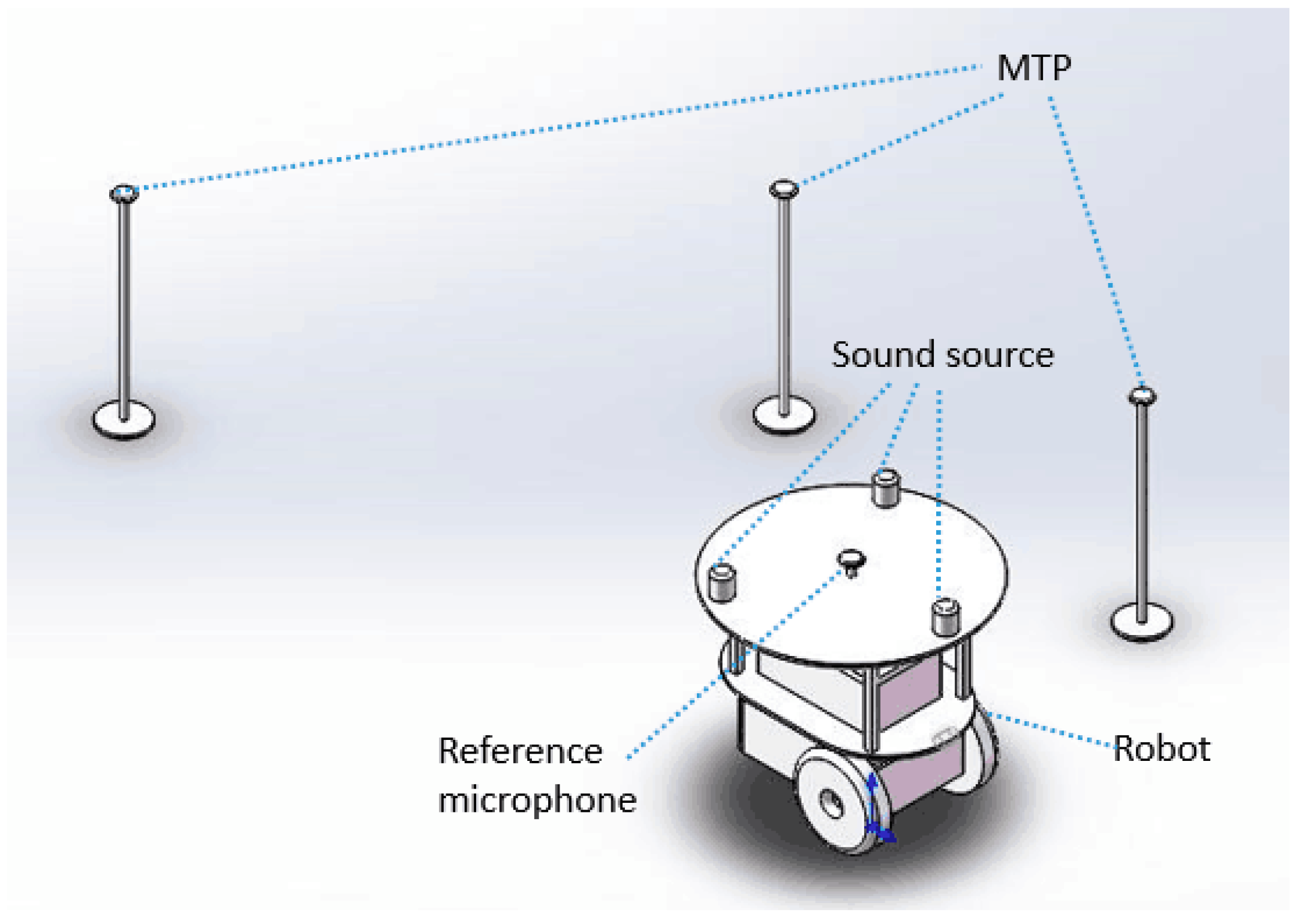
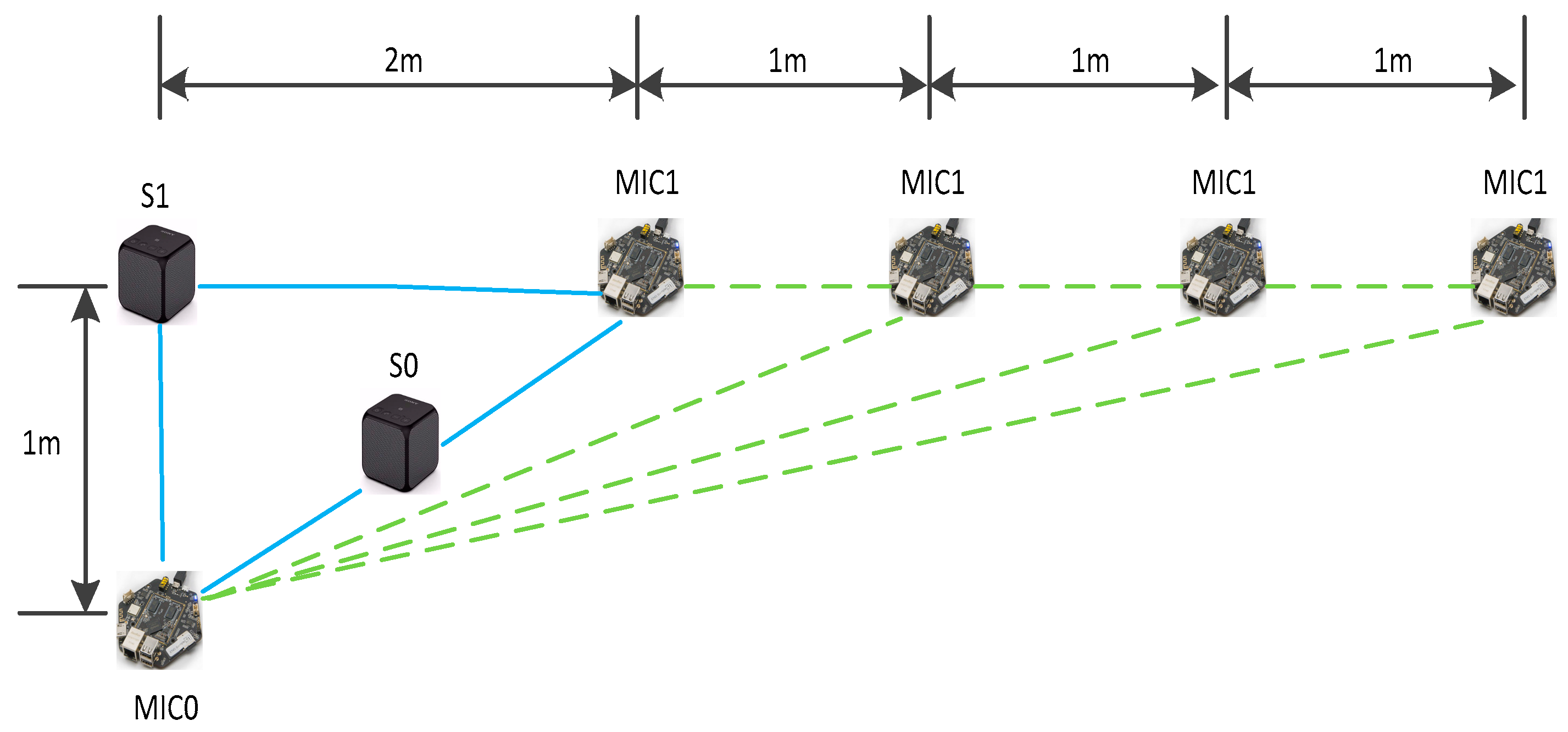
4.2.1. Experiment Setup

Three speakers (s1, s2, and s3) were arranged in an equilateral triangle to form a sound source array mounted on the robot, and the center point of the equilateral triangle coincided with the robot’s center point. There are two advantages to this arrangement of equilateral triangles. One is to ensure uniform dispersion of the sound signals. The other is that if the robot center point is taken as the coordinate origin, it will help with distance calculations and coordinate transformations to reduce the amount of system computation, because of the equal distance from the center point of the robot to the three speakers. All three speakers were connected to the computer via a Bluetooth module to control their sound. At the same time, a microphone was placed at the center of the robot as a reference microphone (m0), also, the distance from it to the three speakers was equal, known, and fixed. The sound source array and the mobile robot for the experiment are shown in Figure 12. The mobile robot Pioneer3-DX was selected as the main operating platform. The robot controller was connected to the Pioneer3-DX through the RS232 serial port. The controlling program sent a control command to the mobile robot according to the robot’s work requirements.

The Seeed ReSpeaker Core v2.0 was selected as the microphone in this paper, as shown in Figure 13. The chip is designed for voice interface applications. It is based on the Quadcore ARM Cortex A7 Rockchip RK3229 and runs at up to 1.5 GHz with 1 GB of Random Access Memory (RAM). It integrates six microphone arrays, and only one of the microphones was used in our case. The sampling rate of the microphone is 16 kHz. ReSpeaker Core v2.0 runs the GNU/Linux operating system. Xshell can control multiple servers at the same time, and only needs to know their IP address. Therefore, this paper mainly used the Xshell software to remotely control the chip under the same Local Area Network (LAN). Compared to traditional microphone systems that collect sound signals, this method does not require the use of many wires to connect devices. The use of the chip greatly reduced the cumbersomeness of the hardware device and improved the efficiency of the experiments.

4.2.2. The Calibration Method

In this experiment, 10 microphones to be positioned (MTP) (m1, m2,…m10) were used as observation landmarks, and they were simultaneously powered, randomly distributed in the environment, and guaranteed to be in the same plane as the sound source array. Since the microphones were remotely controlled by Xshell to collect sound signals, the quality of the network signal and the speed of the signal propagation could lead to measurement errors. In response to this situation, this paper proposed a calibration method to eliminate this error. Take m0 and m1 as an example: we placed a speaker named “calibration sound source (s0)” in the middle of m0 and m1. First s0 sounded, and then s1 sounded. The sound signals received by m0 and m1 are shown in Figure 14. Since the distances between s0, m0, and m1 were equal, the starting positions of the first speech segments of m0 and m1 should be the same. However, analyzing Figure 14, it was found that there were errors. An enlarged view is shown in Figure 15. The difference between the starting positions of the two speech segments was taken as calibration value (e1). There was a difference value (e2) between the starting position of the second speech segment of m0 and m1. The time delay of sound arrival (TDOA1) between m0 and m1 was obtained by Equation (23).

$$\mathrm{TDOA}1=e2-e1$$

(23)

4.2.3. Experiment Results

We programmed the method to acquire sound signals only when the robot stopped. The experimental verification process of the method is as follows:

The robot center point is considered to be the origin. At the initial time, the origin of the robot coordinate system coincides with the origin of the world coordinate system, and the current position of robot is (0, 0). These ten microphones need to be measured one by one to determine the difference in sound time between them and the reference microphone.

• For the first microphone to be positioned (m1), use the calibration method described in Section 4.2.2, to obtain the precise value of time delay of arrival between m0 and m1 (TDOA1).
• Similar to Step 1, first s0 sounds, and then s2 sounds. Finally, TDOA2 between m0 and m1 is obtained. When it is s3, TDOA3 is obtained too.
• Distances between m1 and the three sound sources (d1, d2, d3) is calculated by Equations (6) and (7).
• Evaluate whether m1 is a valid characteristic landmark, and if it is, put m1 into the dataset or abandon it. The evaluation method is described as follows and the evaluation standard value is obtained from actual experimental data analysis in this paper.
• Repeat Steps 1–4 and the other valid microphones are detected in sequence.
• The method of EKF-SLAM based on microphone landmark observations described in Section 3.3 is applied to this procedure.
• The robot insists on moving to the next position and performing the above operations until the end of the experiment.

As shown in Figure 16, there are two sound sources, S0 and S1. S1 is used as the main sound source, and S0 is used as the “calibration sound source”. Also, there are two microphones, MIC0 and MIC1. MIC0 is used as the reference microphone, and MIC1 is used as the microphone to be positioned. The distance between S1 and MIC0 is known for 1 m. Assuming that the distance between MIC1 and S1 is unknown, and it is estimated by the TDOA estimation method introduced in Section 2. Firstly, place MIC1 two meters away from s1, and then move MIC1 in units of one meter to the right to do multiple measurements. Finally, by comparing the estimated distance value with the real, it is found that when the microphone is placed less than 3 m away from the sound source, the acquired sound signal is the most reliable for this method.

Acoustic EKF-SLAM based on microphone landmark observation is summarized in Algorithm 1.

Algorithm 1: Algorithm of Acoustic EKF-SLAM Based on Microphone Landmark Observation.

1: for k = 1,…, 10 do 2:         for I = 1,…, 10 do 3:             for j = 1, 2, 3 do 4:                Sample TDOA(j) using “GCC-PHAT” and “calibration method” 5:                Calculate d(j) using (6), (7) 6:                Evaluate m(i) 7:                if d(j) < 3, 8:                       input m(i) to dataset 9:                else if 10:                      Abandon m(i) 11:            end for 12:          end for 13:          EKF-SLAM based on microphone landmark observation is conducted. 14: end for

To verify the feasibility of the SLAM method presented in this paper, the robot (Pioneer3-DX) was moving through a specifically designed path to avoid some improper situations for TDOA estimation and range-only SLAM, as depicted in Figure 17. The origin was the point where the robot started to move in an $6.05\mathrm{m}\times 4.10\mathrm{m}\times 2.22\mathrm{m}$ experimental area. In the robot coordinate system, three sound sources and the reference microphone at a height of 0.7 m were at s1 = (0, 0.3) m, s2 = (−0.26, −0.15) m, s3 = (0.26, −0.15) m, and m0 = (0, 0) m. Ten microphones to be positioned were dispersedly mounted on the wall in the same plane as the sound source. It can be seen that it was L-shaped. The calibration speaker can be moved when needed. The robot stopped at 10 waypoints to record the acoustic data. It stopped for approximately 120 s to ensure the recording of the sound signal. The speed of robot was fixed when moving.

The SLAM results are shown in Figure 18. In Figure 18a, the red, solid line represents the robot’s planned trajectory (actual trajectory), and the red star points represent microphones that were distributed in an L-shape in the environment, that is, the actual location of the feature landmarks; The blue, dotted line represents the robot’s estimated path trajectory, and the blue circles represent the estimated location of the feature landmarks. By comparing the robot’s real movement trajectory with the trajectory estimated by the EKF-SLAM algorithm regarding the microphones as landmarks, it was found that the two are basically coincident. At the same time, comparing the actual location of the feature landmarks in the environment with the estimated location, it can also be found that the two are basically coincident. However, there was a small difference between the estimated location and the actual location of robots and landmarks. Figure 18b,c show the error analysis of the experimental results.

Table 3. Localization results of a mobile robot. X-error: the error of the robot’s positioning in the x-axis direction. Y-error: the error of the robot’s positioning in the y-axis direction.

	Actual Position	Estimated Position	x-Error	y-Error
Robot’s Position	(0, 0)	(0, 0)	0	0
	(0, 0.586)	(0, 0.586)	0	0
	(0, 1.172)	(0.021, 1.177)	0.021	0.005
	(0, 1.758)	(0.116, 1.806)	0.116	0.048
	(0, 2.344)	(0.185, 2.400)	0.185	0.056
	(0, 2.930)	(0.187, 3.045)	0.187	0.115
	(0, 3.516)	(0.201, 3.643)	0.201	0.127
	(0.586, 3.516)	(0.785, 3.646)	0.199	0.130
	(1.172, 3.516)	(1.371, 3.646)	0.199	0.130
	(1.758, 3.516)	(1.840, 3.646)	0.082	0.130
Standard Deviation			0.132	0.082

and

Table 4. Localization results of landmarks. X-error: the error of the landmarks’ positioning in the x-axis direction. Y-error: the error of the landmarks’ positioning in the y-axis direction.

	Actual Position	Estimated Position	x-Error	y-Error
Landmarks	(−1.775, 0.135)	(−1.788, 0.114)	0.013	0.249
	(−1.775, 1.157)	(−1.646, 1.347)	0.129	0.190
	(−1.775, 1.833)	(−1.606, 1.993)	0.169	0.160
	(−1.775, 2.735)	(−1.579, 2.873)	0.196	0.138
	(−1.775, 4.092)	(−1.568, 4.234)	0.207	0.142
	(−0.915, 5.479)	(−0.712, 5.617)	0.203	0.138
	(−0.125, 5.479)	(0.087, 5.607)	0.212	0.128
	(0.695, 5.479)	(0.898, 5.598)	0.203	0.119
	(−1.775, 5.187)	(−1.554, 5.332)	0.221	0.145
	(1.685, 5.479)	(1.887, 5.589)	0.202	0.110
Standard Deviation			0.195	0.169

show the actual and estimated position for the robot and landmarks, and by comparing them, the standard deviation of the robot’s position and the landmarks’ position are calculated. A very important feature of sound signals are that they are easily affected by environmental noise. The result of this experiment is based on taking into account the actual environmental noise and reverberation. Since this paper uses the GCC method to estimate the TDOA, both environmental noise and reverberation were well suppressed. From the results, it can be seen that the feasibility and effectiveness of the proposed method are well verified.

5. Conclusions

This paper considers the EKF-SLAM for mobile robots based on microphone landmark observations. A kinematic analysis of the mobile robot was conducted and a kinematic model was established. The method of microphone localization based on sound source array in the auditory field was described, and it was combined with the EKF-SLAM algorithm to solve the SLAM problem of the mobile robot. The observation model was established based on microphone landmark observation. In addition, this paper also discussed the advantages and novelty of sound sources and microphones used as external sensors for the SLAM problem compared with traditional sensors such as laser radar. In this paper, the effectiveness and the robustness of the EKF-SLAM based on microphone landmark observation is demonstrated through simulation and experimental tests from the theoretical and practical perspective, respectively. It should be pointed out that this method can only realize the localization of landmarks in two-dimensional planes, and there are problems such as the missing of environmental features and low detection accuracy. To achieve the SLAM of mobile robots faster and more accurately, applying a method of microphone localization in a three-dimensional space in SLAM is still a work to be studied in the future.

References

1. Cadena, C.; Carlone, L.; Carrillo, H. Past, Present, and Future of Simultaneous Localization and Mapping: Toward the Robust-Perception Age. IEEE Trans. Robot. 2016, 32, 1309–1332. [Google Scholar] [CrossRef]
2. Jingwen, L.; Shiyin, Q. A fast algorithm of slam based on combinatorial interval filters. IEEE Access 2018, 6, 28174–28192. [Google Scholar]
3. Luo, J.; Qin, S. A fast algorithm of simultaneous localization and mapping for mobile robot based on ball particle filter. IEEE Access 2018, 6, 20412–20429. [Google Scholar] [CrossRef]
4. Norgren, P.; Skjetne, R. A multibeam-based slam algorithm for iceberg mapping using auvs. IEEE Access 2018, 6, 26318–26337. [Google Scholar] [CrossRef]
5. Grisetti, G.; KuMmerle, R.; Stachniss, C.; Burgard, W. A tutorial on graph-based slam. IEEE Intell. Transp. Syst. Mag. 2010, 2, 31–43. [Google Scholar] [CrossRef]
6. Lowry, S. Visual place recognition: A survey. IEEE Trans. Robot. 2016, 32, 1–19. [Google Scholar] [CrossRef]
7. Davison, A.J.; Reid, I.D.; Molton, N.D.; Stasse, O. Monoslam: Real-time single camera slam. IEEE Trans. Pattern Anal. Mach. Intell. 2007, 29, 1052–1067. [Google Scholar] [CrossRef] [PubMed]
8. Clipp, B.; Lim, J.; Frahm, J.M.; Pollefeys, M. Parallel, real-time visual SLAM. In Proceedings of the IEEE/RSJ International Conference on Intelligent Robots & Systems, Taipei, Taiwan, 18–22 October 2010; pp. 3961–3968. [Google Scholar]
9. Blösch, M.; Weiss, S.; Scaramuzza, D.; Siegwart, R. Vision based MAV navigation in unknown and unstructured environments. In Proceedings of the IEEE International Conference on Robotics & Automation, Anchorage, AK, USA, 3–7 May 2010; pp. 21–28. [Google Scholar]
10. Gao, L.; Yuan, P.; Wang, T.; Shi, Z.; Ji, X. New research on SLAM algorithm based on feature matching. In Proceedings of the 2017 2nd International Conference on Advanced Robotics and Mechatronics (ICARM), Hefei, China, 27–31 August 2017; pp. 1–6. [Google Scholar]
11. Esparza-Jiménez, J.; Devy, M.; Gordillo, J. Visual ekf-slam from heterogeneous landmarks. Sensors 2016, 16, 489. [Google Scholar] [CrossRef]
12. Evers, C.; Naylor, P.A. Acoustic slam. IEEE/ACM Trans. Audio Speechand Lang. Process. 2018, 26, 1484–1498. [Google Scholar] [CrossRef]
13. Krekovic, M.; Dokmanic, I.; Vetterli, M. EchoSLAM: Simultaneous localization and mapping with acoustic echoes. In Proceedings of the IEEE International Conference on Acoustics 2016, Shanghai, China, 20–25 March 2016; pp. 11–15. [Google Scholar]
14. Huang, J.; Kume, K.; Saji, A.; Nishihashi, M.; Watanabe, T.; Martens, W.L. Robotic spatial sound localization and its 3D sound human interface. In Proceedings of the International Symposium on Cyber Worlds, Tokyo, Japan, 6–8 November 2002. [Google Scholar]
15. Okuno, H.G.; Nakadai, K. Robot audition: Its rise and perspectives. In Proceedings of the IEEE International Conference on Acoustic, Brisbane, QLD, Australia, 19–24 April 2015; pp. 5610–5614. [Google Scholar]
16. Nakadai, K.; Ince, G.; Nakamura, K.; Nakajima, H. Robot audition for dynamic environments. In Proceedings of the IEEE International Conference on Signal Processing, Hong Kong, China, 12–15 August 2012; pp. 125–130. [Google Scholar]
17. Nadiri, O.; Rafaely, B. Localization of multiple speakers under high reverberation using a spherical microphone array and the direct-path dominance test. IEEE/ACM Trans. Audio Speech Lang. Process. 2014, 22, 1494–1505. [Google Scholar] [CrossRef]
18. Evers, C.; Moore, A.H.; Naylor, P.A. Localization of moving microphone arrays from moving sound sources for robot audition. In Proceedings of the 2016 24th European Signal Processing Conference (EUSIPCO), Budapest, Hungary, 29 August–2 September 2016; pp. 1008–1012. [Google Scholar]
19. Valin, J.M. Enhanced robot audition based on microphone array source separation with post-filter. In Proceedings of the 2004 IEEE/RSJ International Conference on Intelligent Robots and Systems (IROS) (IEEE Cat. No.04CH37566), Sendai, Japan, 28 September–2 October 2004; Volume 3, pp. 2123–2128. [Google Scholar]
20. Dokmanic, I.; Daudet, L.; Vetterli, M. How to Localize Ten Microphones in One Fingersnap. In Proceedings of the Signal Processing Conference, Lisbon, Portugal, 1–5 September 2014; pp. 2275–2279. [Google Scholar]
21. Okuno, H.G. Robot Recognizes Three Simultaneous Speech by Active Audition. In Proceedings of the IEEE International Conference on Robotics & Automation, Taipei, Taiwan, 14–19 September 2003; Volume 1, pp. 398–405. [Google Scholar]
22. Nakajima, H.; Nakadai, K.; Hasegawa, Y.; Tsujino, H. Blind source separation with parameter-free adaptive step-size method for robot audition. IEEE Trans. Audio Speech Lang. 2010, 18, 1476–1485. [Google Scholar] [CrossRef]
23. Evers, C.; Dorfan, Y.; Gannot, S.; Naylor, P.A. Source tracking using moving microphone arrays for robot audition. In Proceedings of the 2017 IEEE International Conference on Acoustics, Speech and Signal Processing (ICASSP), New Orleans, LA, USA, 5–9 March 2017; pp. 6145–6149. [Google Scholar]
24. Knapp, C.; Carter, G. The generalized correlation method for estimation of time delay. IEEE Trans. Acoust. Speech Signal Process. 1976, 24, 320–327. [Google Scholar] [CrossRef]
25. Omologo, M.; Svaizer, P. Acoustic source location in noisy and reverberant environment using csp analysis. In Proceedings of the ICASSP IEEE International Conference on Acoustics, Speech and Signal Processing, Atlanta, GA, USA, 7–10 May 1996; Volume 2, pp. 921–924. [Google Scholar]
26. Dvorkind, T.G.; Gannot, S. Time difference of arrival estimation of speech source in a noisy and reverberant environment. Signal Process. 2005, 85, 177–204. [Google Scholar] [CrossRef]
27. Ali, S. An application of passive human—Robot interaction: Human tracking based on attention distraction. Syst. Man Cybern. Part A Syst. Hum. IEEE Trans. 2002, 32, 248–259. [Google Scholar]
28. Hu, J.S.; Chan, C.Y.; Wang, C.K.; Lee, M.T.; Kuo, C.Y. Simultaneous Localization of a Mobile Robot and Multiple Sound Sources Using a Microphone Array. In Proceedings of the IEEE International Conference on Robotics & Automation, Kobe, Japan, 12–17 May 2009; pp. 29–34. [Google Scholar]
29. Hu, J.S.; Yang, C.H.; Wang, C.K. Estimation of Sound Source Number and Directions under a Multi-source Environment. In Proceedings of the IEEE/RSJ International Conference on Intelligent Robots & Systems, St. Louis, MO, USA, 11–15 October 2009; pp. 181–186. [Google Scholar]
30. Bailey, T.; Nieto, J.; Guivant, J.; Stevens, M.; Nebot, E. Consistency of the EKF-SLAM Algorithm. In Proceedings of the 2006 IEEE/RSJ International Conference on Intelligent Robots and Systems, Beijing, China, 9–13 October 2006; pp. 3562–3568. [Google Scholar]
31. Jianjun, Y.; Yingkun, Z.; Xiaogang, R.; Yongfang, S. Implementation of an improved UKF algorithm in Electronic whiteboard positioning. In Proceedings of the 26th Chinese Control and Decision Conference (2014 CCDC), Changsha, China, 31 May–2 June 2014; pp. 3824–3828. [Google Scholar]
32. Su, X.; Yan, J.; Yan, S. A UKF algorithm with two arrays in bearings-only tracking. In Proceedings of the 2011 4th International Congress on Image and Signal Processing, Shanghai, China, 15–17 October 2011; pp. 2709–2712. [Google Scholar]
33. Grisetti, G.; Stachniss, C.; Burgard, W. Improving Grid-based SLAM with Rao-Blackwellized Particle Filters by Adaptive Proposals and Selective Resampling. In Proceedings of the 2005 IEEE International Conference on Robotics and Automation, Barcelona, Spain, 18–22 April 2005; pp. 2432–2437. [Google Scholar]
34. He, H.; Jia, Y.; Sun, L. Simultaneous Location and Map Construction Based on RBPF-SLAM Algorithm. In Proceedings of the 2018 Chinese Control and Decision Conference (CCDC), Shenyang, China, 9–11 June 2018; pp. 4907–4910. [Google Scholar]
35. Li, Q.; Wang, Y.; Huang, Y.; Huang, X. Research on Four-Wheeled Indoor Mobile Robot SLAM Based on RBPF Algorithm. In Proceedings of the 2018 IEEE International Conference of Intelligent Robotic and Control Engineering (IRCE), Lanzhou, China, 24–27 August 2018; pp. 24–28. [Google Scholar]
36. Hentout, A.; Beghni, A.; Benahmed Nourine, A.; Maoudj, A.; Bouzouia, B. Mobile robot rbpf-slam with lms sensor in indoor environments application on robuTER robot. In Proceedings of the 2017 5th International Conference on Electrical Engineering—Boumerdes (ICEE-B), Boumerdes, Algeria, 29–31 October 2017; pp. 1–6. [Google Scholar]
37. Kurt-Yavuz, Z.; Yavuz, S. A comparison of EKF, UKF, FastSLAM2.0, and UKF-based FastSLAM algorithms. In Proceedings of the 2012 IEEE 16th International Conference on Intelligent Engineering Systems (INES), Lisbon, Portugal, 13–15 June 2012; pp. 37–43. [Google Scholar]
38. López, E.; García, S.; Barea, R.; Bergasa, L.; Molinos, E.; Arroyo, R.; Romera, E.; Pardo, S. A Multi-Sensorial Simultaneous Localization and Mapping (SLAM) System for Low-Cost Micro Aerial Vehicles in GPS-Denied Environments. Sensors 2017, 17, 802. [Google Scholar] [CrossRef] [PubMed]
39. Cho, H.; Kim, E.K.; Kim, S. Indoor SLAM application using geometric and ICP matching methods based on line features. Robot. Auton. Syst. 2018, 100, 206–224. [Google Scholar] [CrossRef]
40. Mingjie, D.; Wusheng, C.; Bin, F. Underwater Matching Correction Navigation Based on Geometric Features Using Sonar Point Cloud Data. Sci. Program. 2017, 1, 1–10. [Google Scholar]
41. Sun, Q.S.Q.; Wang, H.W.H.; Shen, X.S.X.; Ning, W.N.W.; Fu, X.F.X. Research on the statistical modeling and simulation for interface reverberation. In Proceedings of the 2010 3rd International Conference on Computer Science and Information Technology, Chengdu, China, 9–11 July 2010; pp. 566–570. [Google Scholar]
42. Paik, H.; Sastry, N.N.; Santiprabha, I. Effectiveness of noise jamming with White Gaussian Noise and phase noise in amplitude comparison monopulse radar receivers. In Proceedings of the 2014 IEEE International Conference on Electronics, Computing and Communication Technologies (CONECCT), Bangalore, India, 6–7 January 2014; pp. 1–5. [Google Scholar]
43. Millioz, F.; Martin, N. Estimation of a white Gaussian noise in the Short Time Fourier Transform based on the spectral kurtosis of the minimal statistics: Application to underwater noise. In Proceedings of the 2010 IEEE International Conference on Acoustics, Speech and Signal Processing, Dallas, TX, USA, 14–19 March 2010; pp. 5638–5641. [Google Scholar]
44. Vargas-Rubio, J.G.; Santhanam, B. On the multiangle centered discrete fractional Fourier transform. IEEE Signal Process. Lett. 2005, 12, 273–276. [Google Scholar] [CrossRef]
45. Ersoy, O.K. A comparative review of real and complex Fourier-related transforms. Proc. IEEE 1994, 82, 429–447. [Google Scholar] [CrossRef]
46. Ojha, S.; Srivastava, P.D. New class of sequences of fuzzy numbers defined by modulus function and generalized weighted mean. arXiv, 2016; arXiv:1602.03747. [Google Scholar]
47. Yang, Y.; Liu, G. Multivariate time series prediction based on neural networks applied to stock market. In Proceedings of the 2001 IEEE International Conference on Systems, Man and Cybernetics. e-Systems and e-Man for Cybernetics in Cyberspace (Cat.No.01CH37236), Tucson, AZ, USA, 7–10 October 2001; Volume 4, p. 2680. [Google Scholar]
48. Syeda, M.; Zhang, Y.Q.; Pan, Y. Parallel granular neural networks for fast credit card fraud detection. 2002 IEEE World Congress on Computational Intelligence. In Proceedings of the 2002 IEEE International Conference on Fuzzy Systems. FUZZ-IEEE′02. Proceedings (Cat. No.02CH37291), Honolulu, HI, USA, 12–17 May 2002; Volume 1, pp. 572–577. [Google Scholar]
49. Shaikh-Husin, N.; Hani, M.K.; Seng, T.G. Implementation of recurrent neural network algorithm for shortest path calculation in network routing. In Proceedings of the International Symposium on Parallel Architectures, Algorithms and Networks. I-SPAN′02, Makati City, Metro Manila, Philippines, 22–24 May 2002; pp. 355–359. [Google Scholar]
50. Smith, R.; Self, M.; Cheeseman, P. Estimating uncertain spatial relationships in robotics. In Proceedings of the 1987 IEEE International Conference on Robotics and Automation, Raleigh, NC, USA, 31 March–3 April 1987; p. 850. [Google Scholar]
51. Choi, J.; Choi, M.; Chung, W.K.; Choi, H.T. Data association using relative compatibility of multiple observations for EKF-SLAM. Intell. Serv. Robot. 2016, 9, 177–185. [Google Scholar] [CrossRef]
Figure 1. Reference frame of the system and the main components.
Applsci 09 01352 g001
Figure 2. A part of a sound signal waveform received by two microphones (m0 and m1). The sound signal was received by m0 when t was 14.458 s; the sound signal was received by m1 when t was 14.45 s.
Applsci 09 01352 g002
Figure 3. Time delay of arrival (TDOA) estimating based on the generalized cross-correlation (GCC)-phase transformation (PHAT) methods. The sound signal waveform reached the peak when t was 0.01 s.
Applsci 09 01352 g003
Figure 4. Microphone localization processing chain. MTP: microphone to be positioned.
Applsci 09 01352 g004
Figure 5. Schematic model of the simultaneous localization and mapping (SLAM) problem.
Applsci 09 01352 g005
Figure 6. Kinematic model of the mobile robot.
Applsci 09 01352 g006
Figure 7. Observation model of the mobile robot. The blue dots marked numbers s1–s3 are the sound sources. The red pentagram marked M is the reference microphone and the white triangles marked numbers m1–m3 are the MTPs.
Applsci 09 01352 g007
Figure 8. Extended Kalman filter (EKF)-SLAM processing flow chart.
Applsci 09 01352 g008
Figure 9. Simulation results for SLAM with no noise in the sound signal: (a) EKF-SLAM for a mobile robot based on microphone landmark observations; (b) robot position errors in the x- and y-directions; and (c) landmark position errors in the x- and y-directions.
Applsci 09 01352 g009aApplsci 09 01352 g009b
Figure 10. Simulation results for SLAM with a signal-to-noise (SNR) of 65 (dB) in the distance data: (a) EKF-SLAM for a mobile robot based on microphone landmark observations; (b) robot position errors in the x- and y-directions; and (c) landmark position errors in the x- and y-directions.
Applsci 09 01352 g010
Figure 11. Simulation results for SLAM with an SNR of 50(dB) in the distance data: (a) EKF-SLAM for the mobile robot based on microphone landmark observations; (b) robot position errors in the x- and y-directions; and (c) landmark position errors in the x- and y-directions.
Applsci 09 01352 g011
Figure 12. Positional relationship of the sound source array, reference microphone, and mobile robot.
Applsci 09 01352 g012
Figure 13. Seeed ReSpeaker Core v2.0 consisting of six microphones. The microphone circled in red is the one we used in our experiments.
Applsci 09 01352 g013
Figure 14. The waveform of sound signals received by m0 and m1.
Applsci 09 01352 g014
Figure 15. Partially enlarged view of the first speech segments.
Applsci 09 01352 g015
Figure 16. Schematic diagram of the evaluation method.
Applsci 09 01352 g016
Figure 17. Positional relationship of the sound source array, robot, and landmarks for the experiment.
Applsci 09 01352 g017
Figure 18. Experimental result of acoustic EKF-SLAM based on microphone landmark observations: (a) EKF-SLAM for a mobile robot based on microphone landmark observations; (b) robot’s position errors in the x- and y-directions; and (c) landmark position errors in the x- and y-directions.
Applsci 09 01352 g018