An Approach to a Clock Offsets Model for Real-Time PPP Time and Frequency Transfer During Data Discontinuity

Abstract

To resolve the dilemma in any post-processing strategy, i.e., the difficulty of monitoring the real-time time and frequency signals in a timely manner, real-time GPS time and the frequency transfer have recently become trending topics. Unfortunately, data interruption occurs when conducting real-time time transfer, sometimes from unexpected reasons. In this study, to ensure the stability and precision of real-time time transfer, an adaptive prediction model and a between-epoch constraint receiver clock model are applied as the mathematic models. The purpose of prediction is to solve the ambiguity from re-convergence when the data reappear. Moreover, compared to the conventional method, the between-epoch constraint receiver clock model is employed in this study to consider the correlation of epoch-wise clock parameters to avoid wasting useful information. The simulation data and real data are compared to verify the performance of the new approach. The simulation data for 165 days are designed with random daily interruptions of 10, 30, 60 and 90 min. Real data from 12 days is captured from the incomplete data in routine observation records. Ignoring the simulation data and real data, the investigation of six stations shows that the results with the between-epoch constraint receiver clock model were smoother than those with a white noise model. With an adaptive prediction model and the between-epoch constraint receiver clock model, the simulation results illustrate that the average root mean squares (RMS) values of all the stations are significantly reduced, i.e., by 66.03% from 0.43 to 0.14 ns, by 64.91% from 0.44 to 0.15 ns, by 57.47% from 0.43 to 0.18 ns, and by 51.67% from 0.44 to 0.21 ns for the 10, 30, 60 and 90 min data interruptions, respectively. The stability of all the stations is improved by at least 50%. The improvement increases to 100% for short-term stability. The real results show that the stability of four links is boosted by at least 5%. The model proposed in this paper is more effective in producing short-term stability than long-term stability.

1. Introduction

Since its first application in 1980, the global positioning system (GPS) has been recognized as an efficient tool for time and frequency transfer [1]. The GPS technique has been applied for time transfer with pseudo range measurements in the early days, which is referred to as common-view (CV) and all-in-view (AV) [1,2]. Due to the high-precision of the carrier phase measurement, the techniques based on code observations no longer provide the optimal time transfer solutions. Another approach, which could improve TAI (International Atomic Time) time links and TAI computation, was proposed in 2006 [3]; it is referred to as the carrier phase (CP) technique. By virtue of the precise orbit and clock products distributed freely and routinely by the IGS (International GNSS Service), precise point positioning (PPP) is one of the most promising time comparison techniques available, primarily because of its high-accuracy, cost-effectiveness, and global coverage [3,4,5]. PPP time transfer results have been used in TAI at BIPM (Bureau international des poids et mesures) since September 2009, and are involved in over 50% of the more than 70 timing laboratories’ contributions to TAI and UTC (Coordinated Universal Time) [3,6]. The PPP strategy has better short-term stability compared to code-only techniques. The statistical uncertainty is approximately 0.3 ns for PPP links in BIPM circular T, and the frequency comparison is approximately 1 × 10⁻¹⁵ with a 1-d averaging time [6,7]. In recent years, the research community has shown a growing interest in the PPP technique [8,9,10,11].

To meet the increasing requirements of real-time PPP applications, the IGS initiated the IGS Real-Time Pilot Project (IGS-RTPP) in 2007 and provided the precise orbit and clock corrections [12,13,14]. L. Zhang, Yang, Gao, Yao, and Xu (2018) evaluated real-time precise orbits and clock products from different IGS analysis centres (ACs). The results indicated that the root-mean-square error (RMSE) of a satellite orbit ranges from 3.8 cm to 7.5 cm for different real-time service (RTS) products, while the mean standard deviations of errors (STDE) of the satellite clocks range from 1.9 cm to 5.6 cm. These data show that RTS products are suitable for PPP applications. Liu, Zhang, Yuan, and Li (2018) proposed models, algorithms and ionosphere applications of real-time PPP (RT-PPP). Their studies reveal that slant ionosphere delays from RT-PPP are more precise and have a much better convergence performance than those from the carrier-to-code levelling (CCL) method in real-time processing.

Currently, PPP is mainly utilized in post processing as a crucial time transfer technique. A limited number of researchers attach great importance to RT-PPP time transfer techniques [15,16,17], employing continuous observation and products. However, as far as the practical application of RT-PPP time transfer is concerned, the problem is more complicated. There are numerous cases, which will significantly affect statistical uncertainty in RT-PPP time transfer. One case involves a data discontinuity from network problems [18] that leads to product loss or a delay in processing. The data discontinuity will cause a re-convergence of the clock parameters and the ambiguity parameters, or a clock jump. This is true for both static and kinematic models when the clock offset is modelled as white noise. This consequently gives rise to a degradation of the RT-PPP time transfer performance, as evidenced by the fact that ambiguity parameters will be initialized at the time of the data interruption, presenting a strong correlation with clock offset parameters. Until now, there has been no body of literature investigating the problem. These deficiencies of previous studies are the main drivers of this contribution, in which we demonstrate the efficiency of the clock model for instantly recovering clock offset, avoiding re-convergence when there is a data discontinuity in the RT-PPP time transfer data processing.

The organization of this contribution is as follows. In Section 2, the basic principles of RT-PPP time transfer are briefly reviewed, and we describe in detail how to deal with clock offset re-convergence or parameter estimations from a data discontinuity with the clock offset model. The experimental data and processing strategies are presented in Section 3. The experimental results from applying our approach in clarifying the overall performance in RT-PPP time transfer with a data discontinuity is presented in Section 4. The conclusions are presented in Section 5.

2. Method

The ionosphere-free (IF) equation for the pseudo range and carrier phase observation is first presented. The clock models are then introduced. We end with a detailed description of the RT-PPP time transfer processes used in our approach.

2.1. The Observation Model

In the time community, the equation of the ionosphere-free (IF) pseudo range and carrier-phase observations is linear, and can be written as follows [3]:

$$\{\begin{array}{ll}{P}_{r,IF}^S& ={\rho }_r^S+c·d{t}_r-c·d{t}^S+m{f}_w(e)·Z_w+(d_{r,IF}^S-d_{IF}^S)+{\epsilon }_{r,IF}^S\\ L_{r,IF}^S& ={\lambda }_{IF}^S·{\mathsf{\Phi }}_{r,IF}^S\\ & ={\rho }_r^S+c·d{t}_r-c·d{t}^S+m{f}_w(e)·Z_w+{\lambda }_{IF}^S·(N_{r,IF}^S+b_{r,IF}^S-b_{IF}^S)+{\xi }_{r,IF}^S\end{array}$$

(1)

where r indicates the receiver, S indicates the satellite; $P_{r,IF}^S$ and $L_{r,IF}^S$ denote the pseudo-range and the phase observables in metres, respectively; ${\lambda }_{IF}^S$ is the carrier wavelength when ionosphere-free; ${\mathsf{\Phi }}_{r,IF}^S$ is the original carrier phase measurement in cycles; $\rho$ is the geometric distance in metres; c denotes the speed of light; $d{t}^S$ and $d{t}_r$ are the clock offsets of the satellite and receiver in seconds; e is the elevation angle of the satellite S; $m{f}_w(e)$ refers to wet mapping functions [19]; $Z_w$ represents the zenith wet delay; $d_{r,IF}^S$ and $d_{IF}^S$ are the uncalibrated code delays (UCDs) of the IF model at the receiver and satellite end, respectively; $N_{r,IF}^S$ is an integer itself but is estimated as a floating point number from unmodeled effects; $b_{r,IF}^S$ and $b_{IF}^S$ are the uncalibrated phase delays (UPDs) of the IF model at the receiver and the satellite ends in cycles; and ${\epsilon }_{r,IF}^S$ and ${\xi }_{r,IF}^S$ denote the sum of the measurement noise and the multipath error for the pseudo range and carrier phase observations, respectively. Since $d_{IF}^S$ is absorbed by the satellite clock [20], the clock offset of the receiver $d{\overline{t}}_r$ can be written as follows [8]:

$$d{\overline{t}}_r=d{t}_r+d_{r,IF}^S$$

(2)

The relativistic effects, the Sagnac effect, tidal loadings, the slant hydrostatic delay, satellite and receiver antenna phase centre offsets and variations (PCO and PCV) [21,22], and the phase wind-up must be corrected with an experimental model [5], even though they are not included in (1). Detailed descriptions are listed in

Table 1. Summary of GPS PPP (global positioning system precise point positioning) processing strategies.

Item	Strategies
Estimator	Kalman filtering
Relativistic effect	IERS conventions 2010
Sagnac effect	IERS conventions 2010
Phase wind-up	Corrected by model
Tide displacements	IERS conventions 2010
Tropospheric delay	ZHD: corrected with global pressure and temperature (GPT) model using the formulas of Saastamoninen
	ZWD: estimated as a continuous piecewise linear function (2 h parameter spacing), GMF mapping function
Satellite antenna PCOs and PCVs	IGS “*.atx” file

.

The least square method is a type of mathematical optimization technology. The optimal result is obtained with the constraint of the minimum square sum of the residuals. The corresponding normal equation is used to estimate the unknown parameters as follows:

$$A^{T}PA·\widehat{X}=A^{T}PL$$

(3)

where $\widehat{X}$ denotes the vector of all estimated parameters, including the receiver clock offset, tropospheric zenith delay and phase ambiguity; A is the corresponding design matrix; P is the weight matrix, which is determined by the elevation-dependent model; and L is the difference between the observed quantity and the computed quantity. The equation can be rewritten in the following simple format:

$$N·\widehat{X}=b$$

(4)

where $N$ denotes $A^{T}PA$ and $b$ denotes $A^{T}PL$. The least square method is applied in the adaptive receiver clock prediction model. We introduce the clock model in the next subsection.

2.2. The Clock Model

Generally, the clock offset parameter is estimated using white noise. In this contribution, we estimate the clock offset using the between-epoch constraint model (random-walk model). If the receiver clock offset exists in the IGS clock file, a prior variance is calculated from the known clock offset. If not, the receiver clock offset is calculated using the PPP method and a prior variance is computed according to the Allan variance. Considering the white frequency modulation (WFM) noise $q_1$, the random walk frequency modulation (RWFM) noise $q_2$, and the random run frequency modulation (RRFM) noise $q_3$, we obtain the following equation [23]:

$${\delta }_{Allan}^2\left(\tau \right)=q_1{\tau }^{-1}+\frac{q_2\tau }{3}+\frac{1}{20}{q}_3{\tau }^3$$

(5)

where ${\delta }_{Allan}^2\left(\tau \right)$ is the Allan variance at a time interval of $\tau$; q₁, q₂ and q₃ are estimated first by the least square method; and a prior noise variance $Q_w$ is then determined [24].

In the RT-PPP static mode, the value of the coordinate is known. Additionally, the tropospheric delay can be constrained by a prior value because of its small short-term change. Therefore, the data interruption does not induce any influence on these two parameters. However, as we mentioned previously, the clock offset parameter will re-converge because of the ambiguity in initialization when the data is interrupted. Hence, based on the between-epoch constraint model, an adaptive prediction clock model is applied to mitigate the re-convergence error of the clock offset when experiencing a data discontinuity. A standard model for a clock offset is described as follows:

$$d{\overline{t}}_r=a_0+a_1\left(t_i-t_0\right)+\frac{a_2}{2}{\left(t_i-t_0\right)}^2+{\displaystyle \sum _{l=0}^k{A}_l·\sin (\omega ·t_i+{\phi }_l)}$$

(6)

where $a_0$, $a_1$ and $a_2$ are the coefficients of the low-degree polynomial; t_i is the time at epoch $i$; $A_l$ denotes the coefficients of the periodic functions; $\omega$ is the frequency of the periodic items; and ${\phi }_l$ is the phase deviation of the periodic term.

The first-order, second-order polynomial model is employed in this contribution, and $a_0$, $a_1$ and $a_2$ are estimated as constant parameters using the least square method. Note that the weight of the clock is determined by the corresponding variance. Furthermore, an adaptive prediction model is introduced for predicting the clock offset to ensure the continuity of the clock offset time series. ‘Adaptive’ signifies that the selection of the polynomial model is dynamic, depending on the fitting residuals. A detailed diagram of the adaptive prediction clock model is shown in Figure 1. The frequency spectrum of the clock offset is analysed using a fast Fourier transform (FFT).

The process of the RT-PPP time and frequency transfer using the clock model is shown in Figure 2. It mainly includes two parts, as follows:

(1)

We obtain the observations from the receiver (connected to their time and frequency generator, a 1 PPS signal and a 5/10 MHz frequency signal), broadcast ephemeris and state space representation (SSR) corrections from IGS/ACs [25,26,27].

(2)

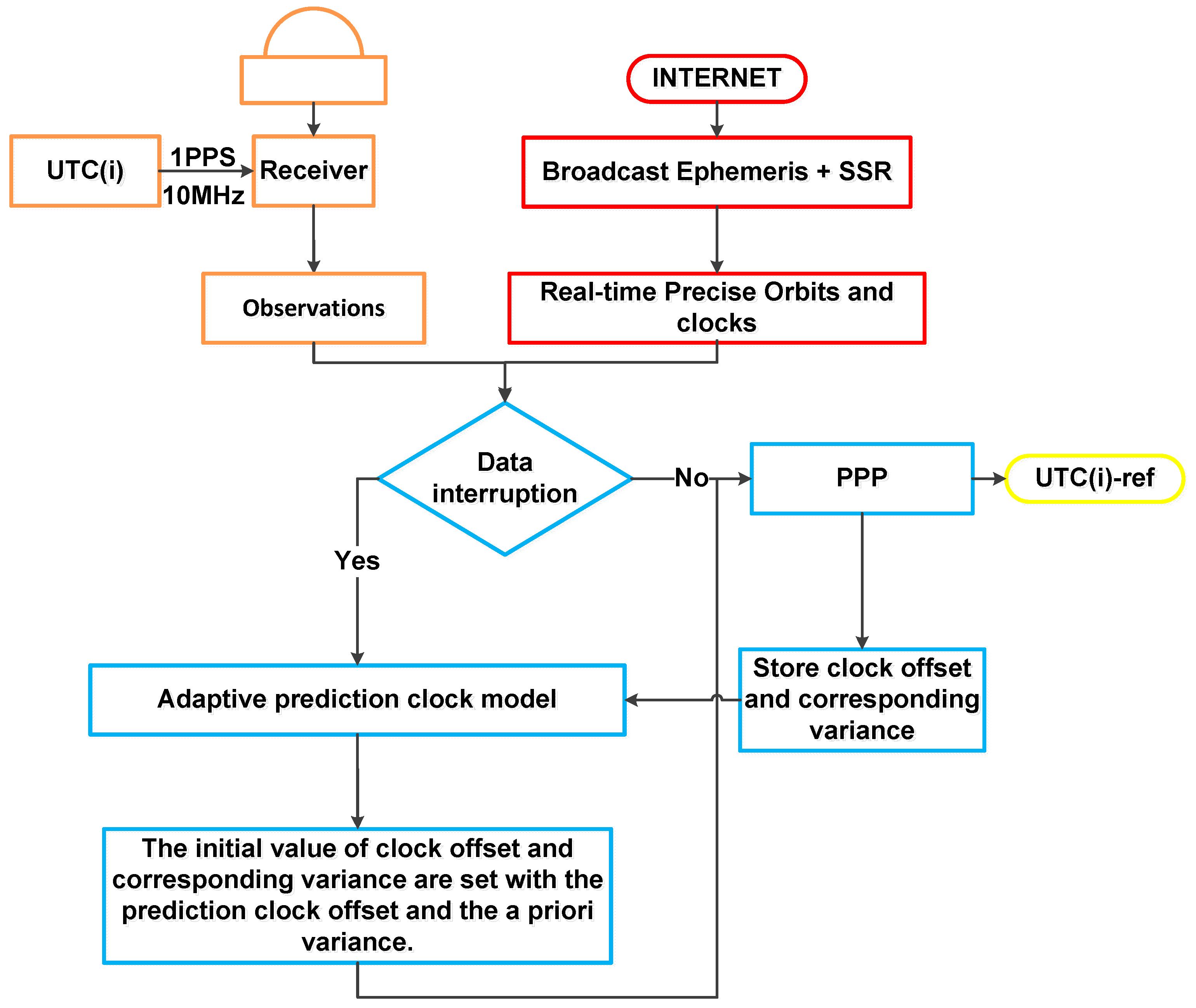
If the data is not interrupted, it will go directly to RT-PPP processing to calculate the difference between the local time UTC (i) and the reference time (ref). Then, the clock offset, and the corresponding variance are stored. We use a sliding window with a window length of 240 data points to store the clock offset data. However, when data interruption occurs, we use the stored clock offset data to calculate the coefficient of the adaptive prediction model, and then predict the clock offset of the current epoch, with the current clock offset as a prior value, while setting the corresponding variance. Importantly, an a priori clock offset of 20 consecutive epochs is set to the predicted clock offset starting from the data, and the products are re-received to help ambiguity parameters to recover quickly and accurately. The detailed variance setting will be described in the next section.

When the difference between the local time and the reference time is calculated in two or more stations simultaneously, the time difference between station A and station B can be expressed as follows:

UTC (i) − UTC (j) = (UTC (i) − ref) − (UTC(j) − ref)

(7)

where ref is the reference time, such as IGST (International GNSS Time); and UTC (i) and UTC (j) are the local times at station A and station B, respectively.

3. Experimental Data and Processing Strategies

In this section, we first describe the datasets of the experiments, including the simulation data and real-time products. The processing strategies are then described in detail.

3.1. Experimental Data Sets

To validate how our approach performs when the data are interrupted during an RT-PPP time and frequency transfer, we sampled observation data every 30 seconds from 6 stations of the IGS network, covering DOY (days of the year) 182–212 in 2018. The detailed information from 6 stations are listed in

Table 2. Details of the selected IGS stations.

Station	Receiver	Antenna	Clock	Distance from BRUX (km)
BRUX	SEPT POLARX4TR	JAVRINGANT_DM	CH1-75A MASER	-
PTBB	SEPT POLARX4TR	LEIAR25.R4 LEIT	H-MASER	454.88
OPMT	ASHTECH Z-XII3T	3S-02-TSADM	UTC(OP)	262.33
WAB2	ASHTECH Z-XII3T	ASH700936F_C	UTC(CH) MASTER	487.20
IENG	ASHTECH Z-XII3T	ASH701945C_M	H-MASER	687.69
NIST	NOV OEM4-G2	NOV702	H-MASER	7365.98

. High-performance receivers have the advantage of being able to perfectly synchronize the internal clock to an external signal source. In this contribution, the experimental data sets are divided into two main parts:

(1)

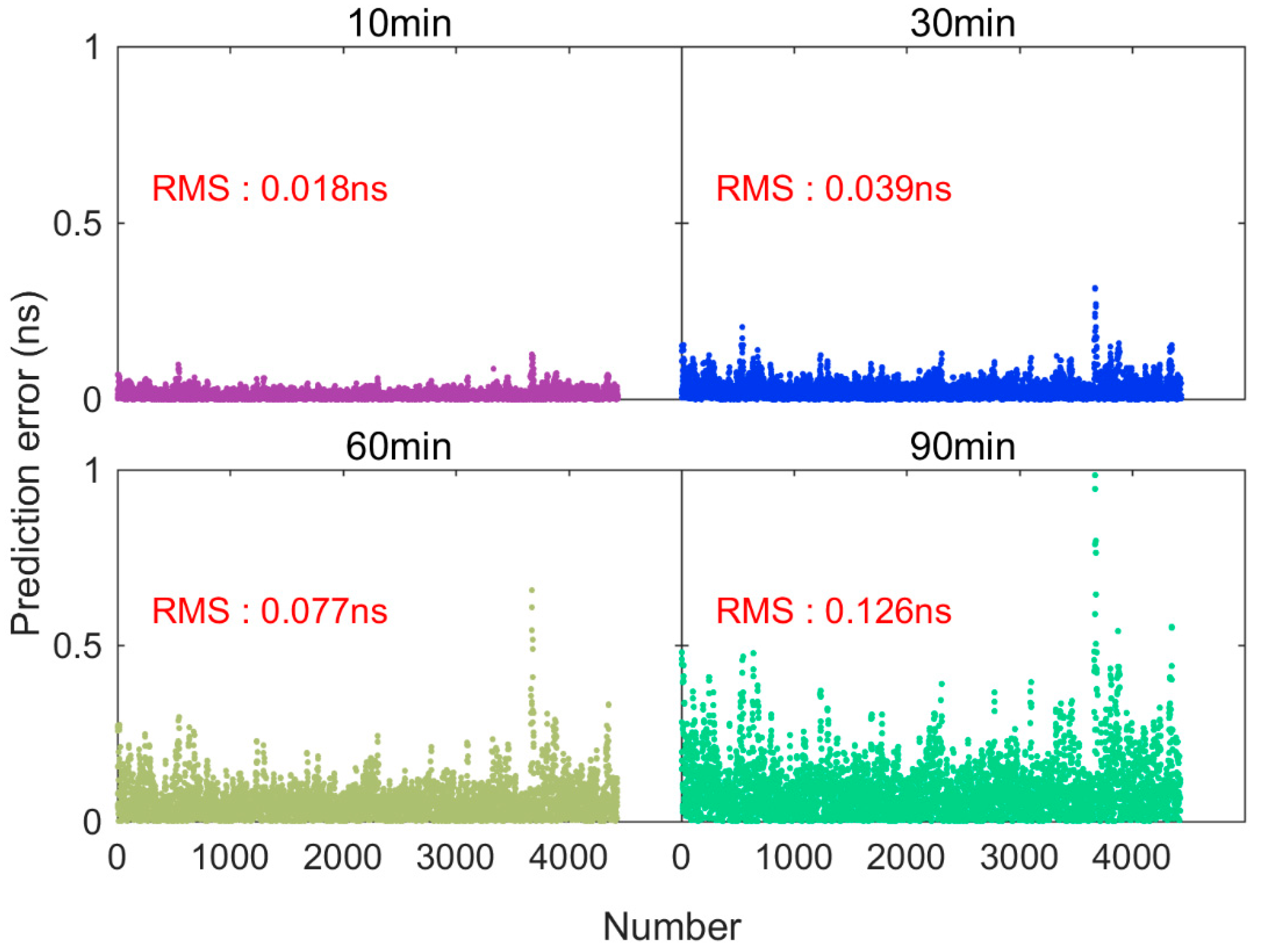
Simulation data: The daily observations and products will be randomly interrupted four times for 10 min, 30 min, 60 min and 90 min, respectively. The precise orbit and clock products released by IGS are utilized in this part.

(2)

Real-time product: The real-time products used in this study were developed by GMV (GMV Aerospace and Defence) (CLK81).

3.2. Processing Strategy

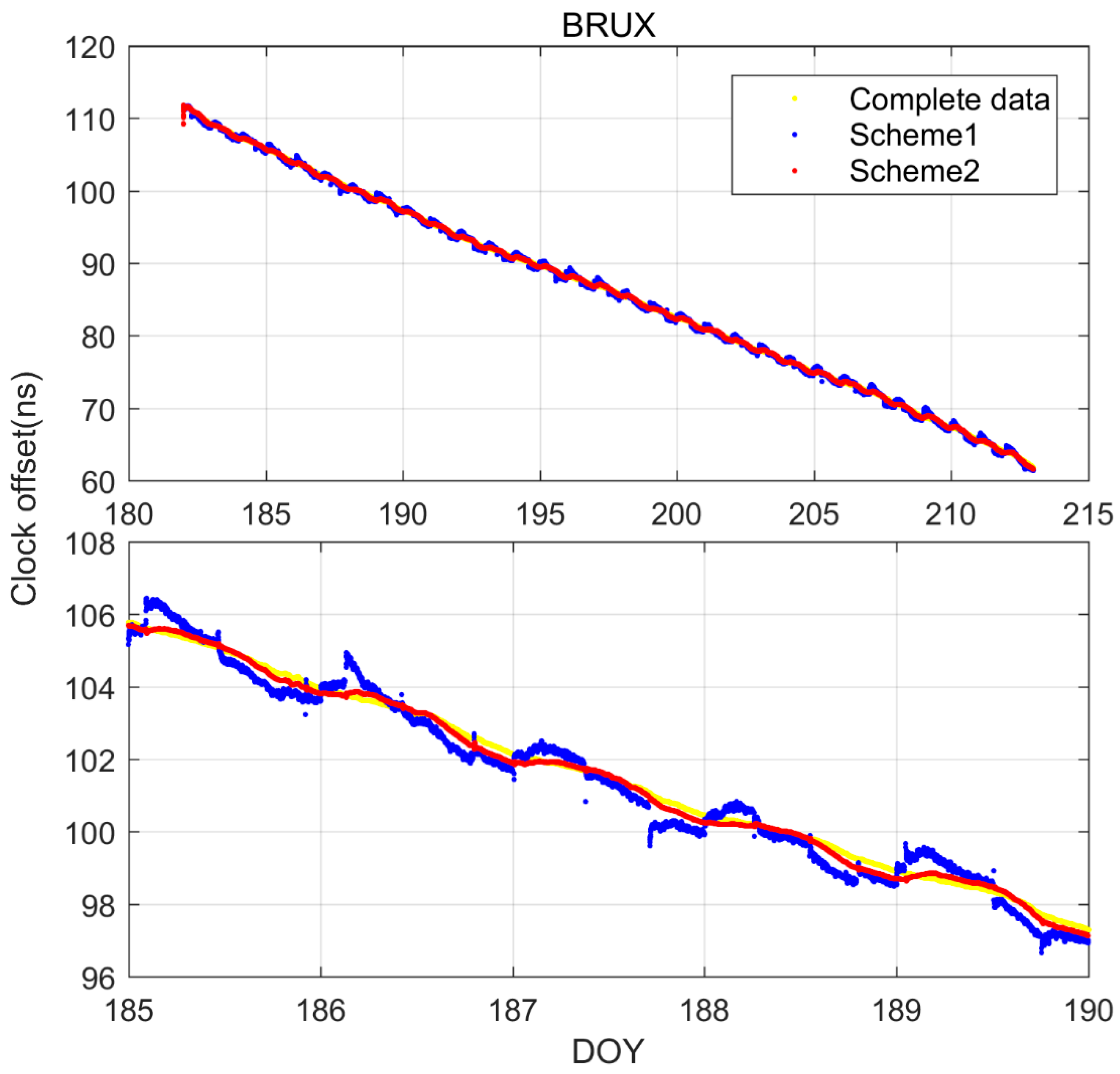
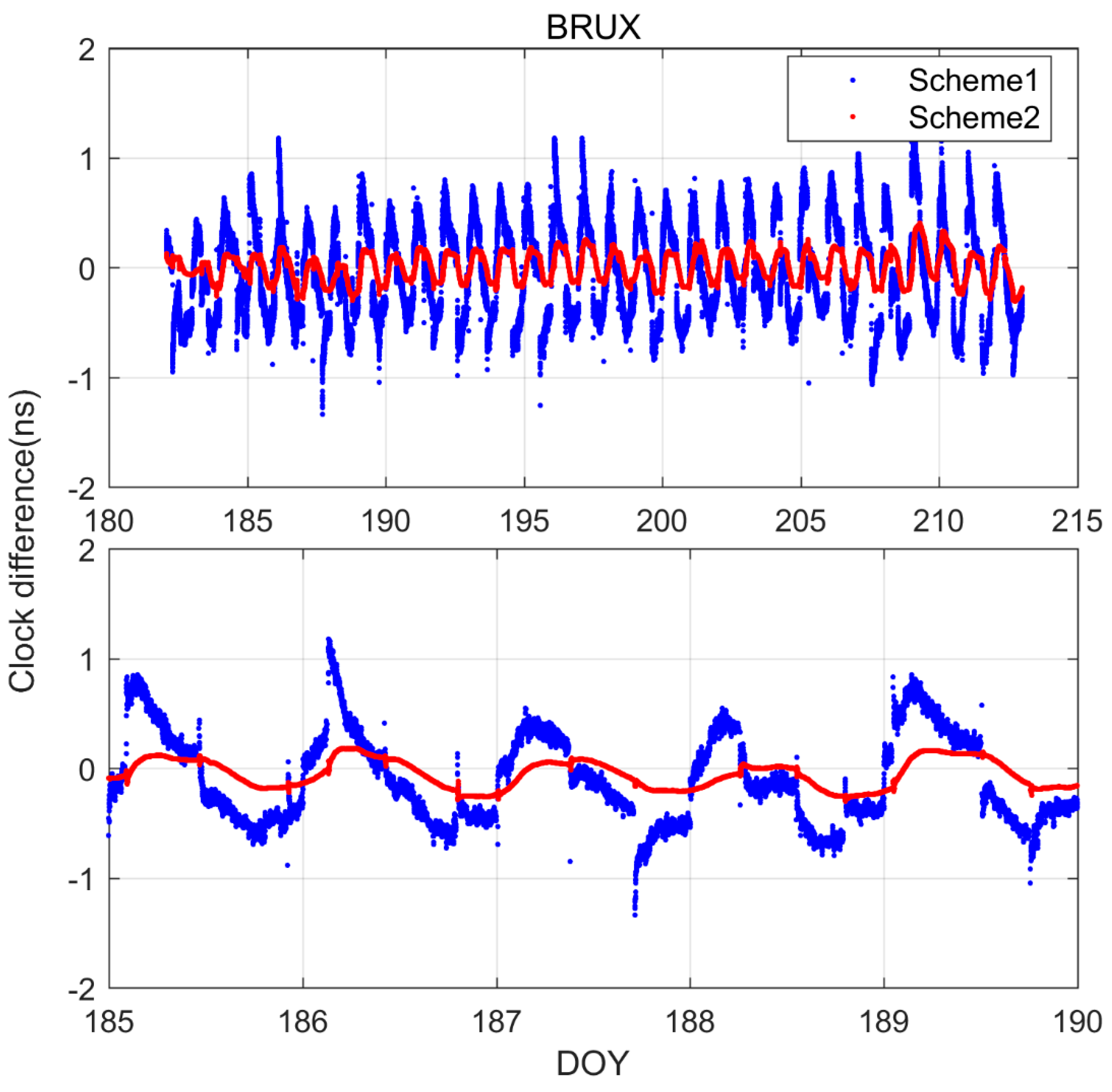
GPS-only RT-PPP static modes were used in our study. GPS precise orbit and clock products and real-time satellite orbit and clock corrections were provided by IGS and GMV (one of the IGS analysis center), respectively. For the data processing, the elevation cutoff angle was set to 10°, and the elevation-dependent weight for the observations with elevations below 30° was applied. The zenith wet delays were estimated as random-walk noise. The float-phase ambiguities were estimated as being constant for each continuous satellite arc. The initial standard deviation values for the GPS carrier phase observations were both set to 0.003 m, while the measurement error ratio between the pseudo range and carrier phase observations was set to 100. In the static PPP mode, the position coordinates were considered to be constants.

In this study, the predicted clock offset is regarded as a prior value when the observation interruption occurs. The strategies of clock offset estimation were divided into two parts:

(1)

Estimate clock offset with a white noise model (marked as scheme 1); and

(2)

Estimate clock offset with the between-epoch constraint model (marked as scheme 2).

The RT-PPP time transfer with data interruption was then investigated using simulation data and real-time data with the two handling schemes.

4. Results and Analysis

We begin this section by determining the prior variance of the predicted clock result, following which we illustrate the numerical results, from which the major findings we identify are also detailed.

We focus first on Figure 3, which depicts the clock offset time series obtained for two different estimation models of the clock offset at station BRUX. The data show that the noise from the clock offset with the between-epoch constraint model is smaller than the clock offset with the white noise model. Hence, the between-epoch constraint model is employed to estimate the clock offset parameter.

To determine the accuracy of the clock offset prediction, 4400 tests were performed. The predicted error was for 10, 30, 60 and 90 min prediction periods. The prediction error of the adaptive clock prediction model at station BRUX is exhibited here in Figure 4 due to the limited space. Furthermore, the root mean squares (RMS) of the predicted errors are presented in

Table 3. The RMS values of the prediction error on six stations (ns).

	10 min	30 min	60 min	90 min
BRUX	0.018	0.039	0.077	0.126
IENG	0.049	0.097	0.182	0.290
NIST	0.025	0.052	0.102	0.166
OPMT	0.029	0.057	0.112	0.183
PTBB	0.024	0.049	0.100	0.159
WAB2	0.035	0.054	0.100	0.152

. Taken together, we make three observations. First, the prediction error is extremely stable, which further explains the reliability of the adaptive clock prediction model. Second, considering the RMS values of the prediction error, they follow an order of increasing trend when the prediction period ranges from 10 min to 90 min, thereby indicating that our approach for short-term data interruption will obtain better results, but that this is not the case for long-term data interruption. We do not conceal this restriction. We recommend that the clock offset parameter be reinitialized if the data is interrupted for a long period. Third, the prediction accuracy of all the stations present similar qualities for the same prediction periods. Hence, the variance values will be set from a prior variance in this contribution.

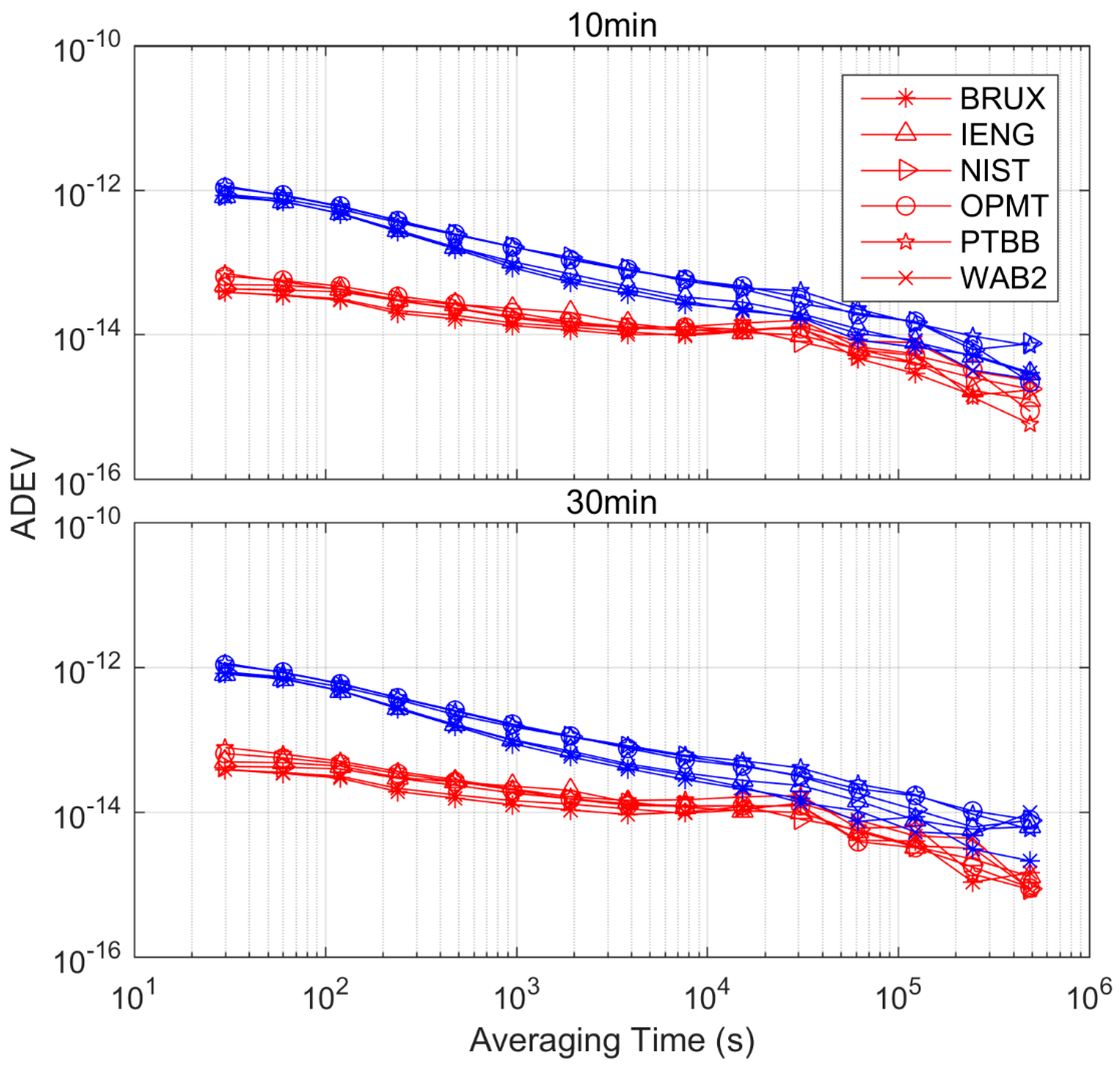
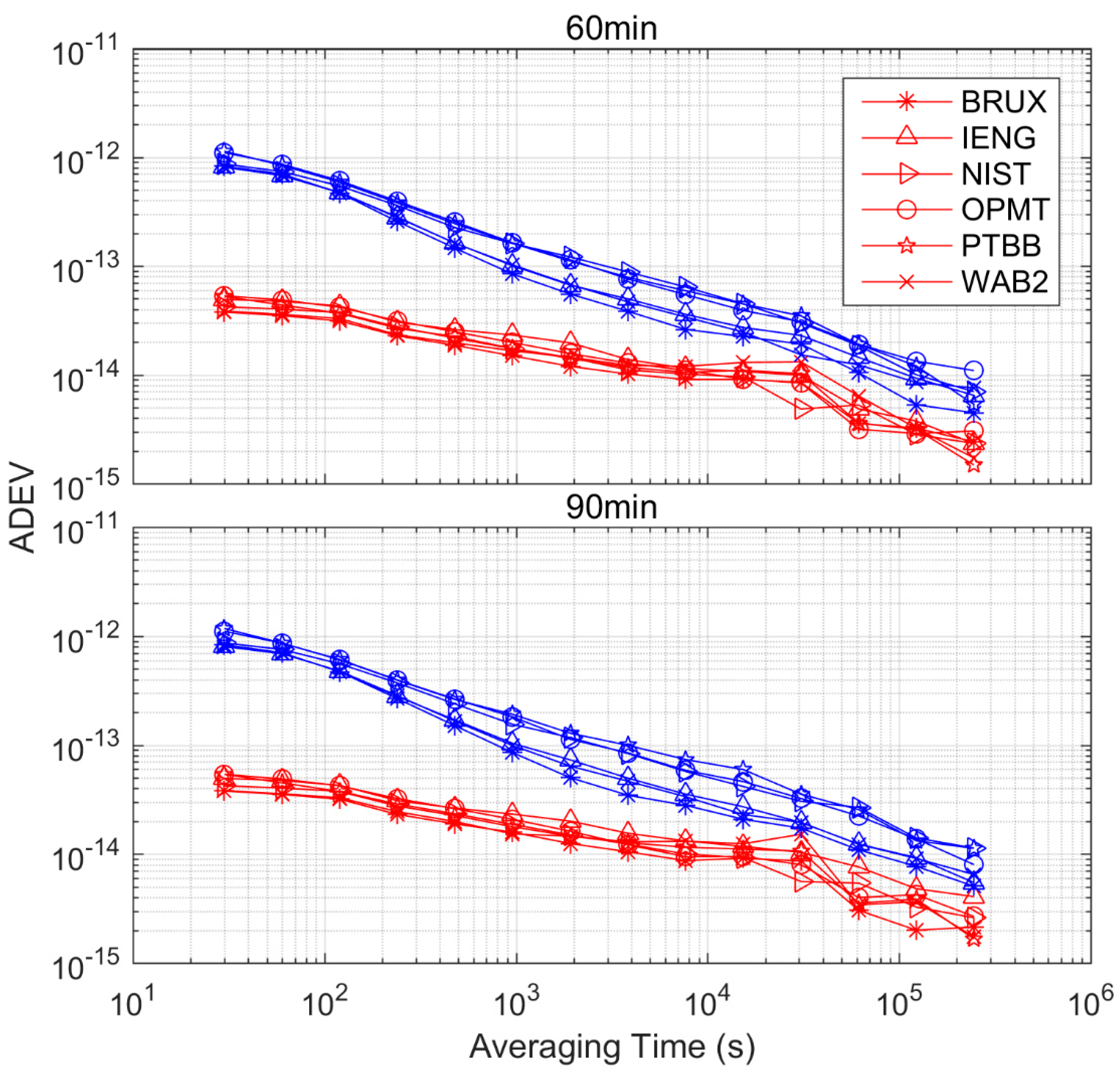
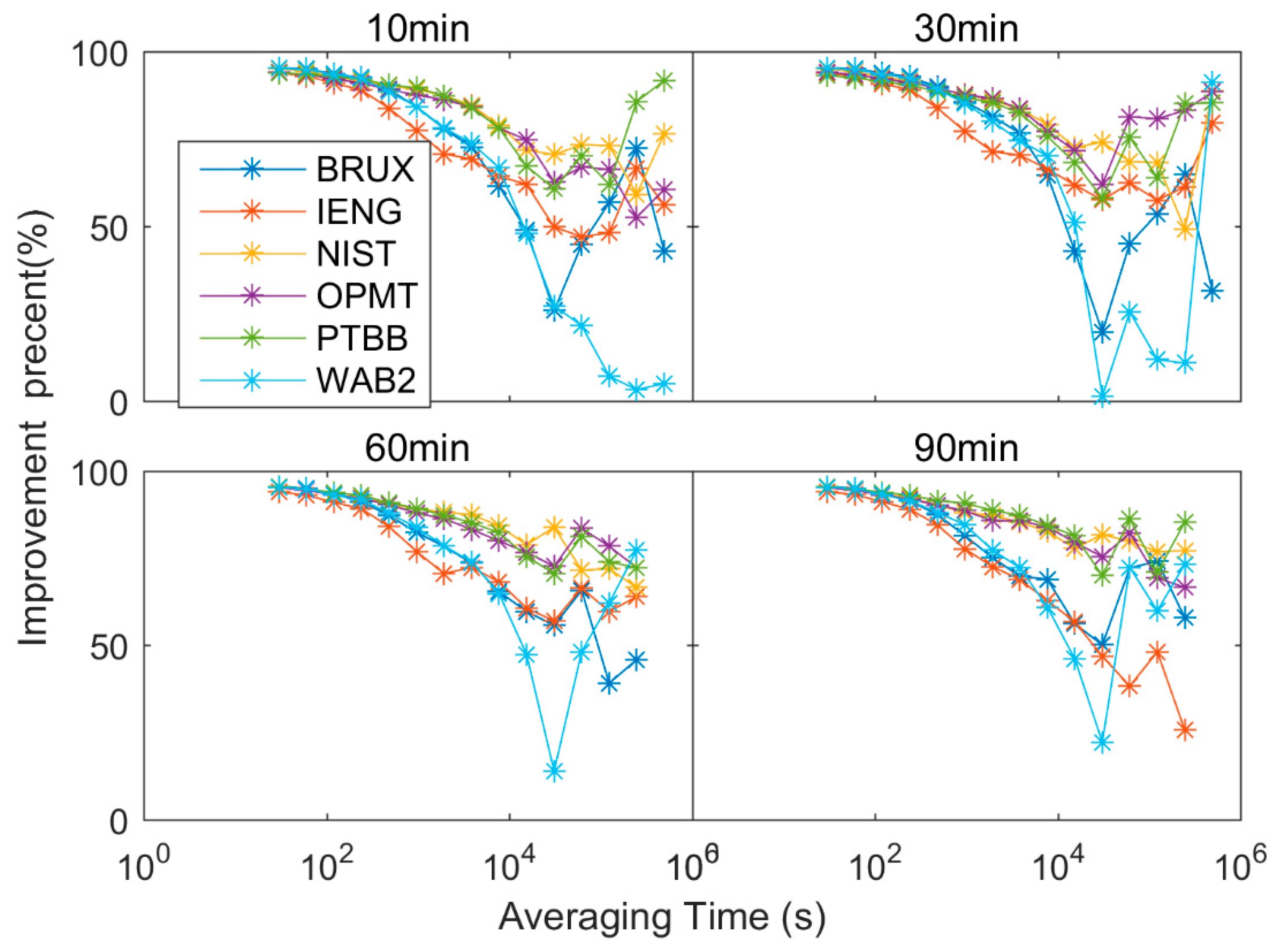
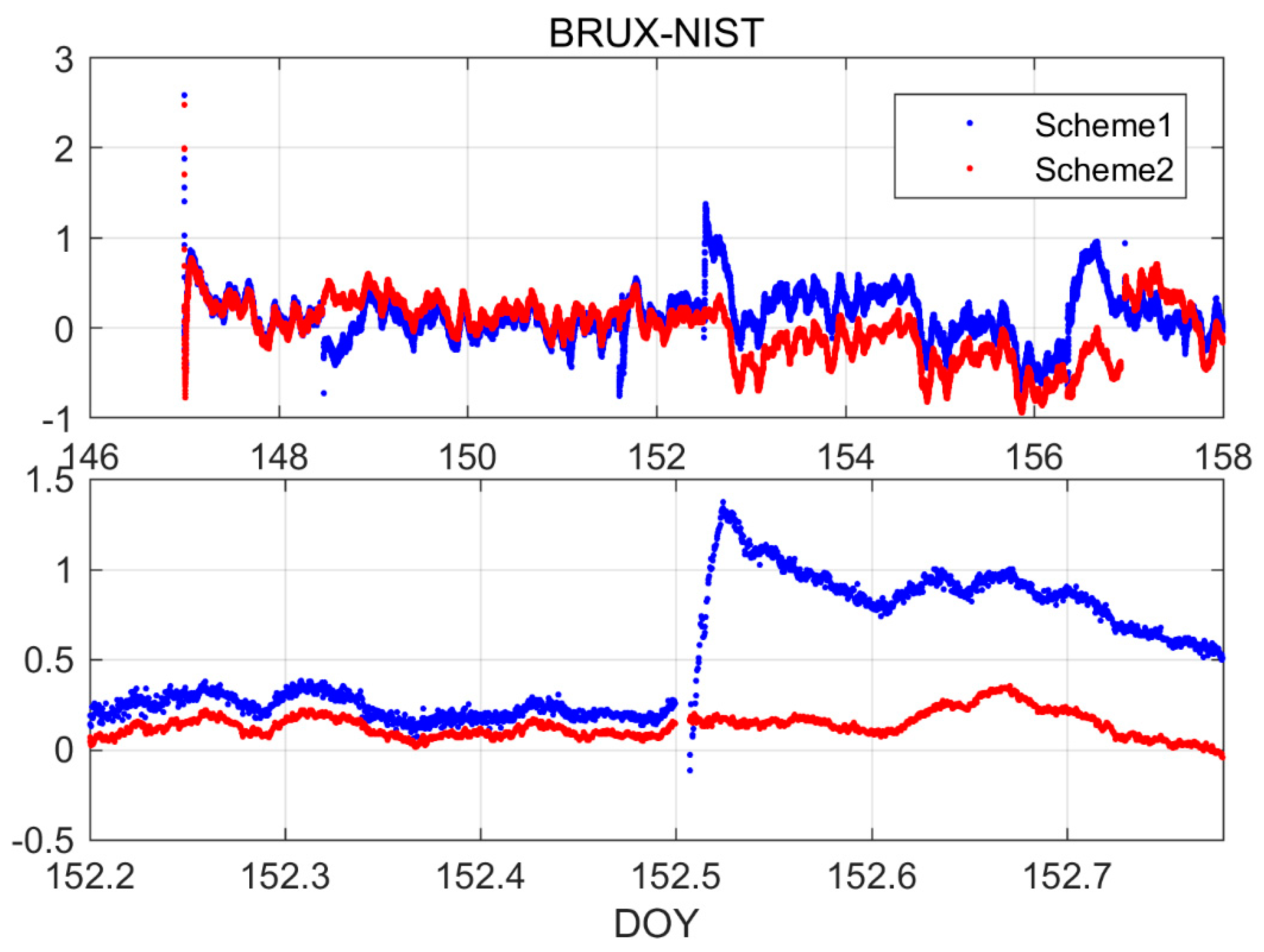
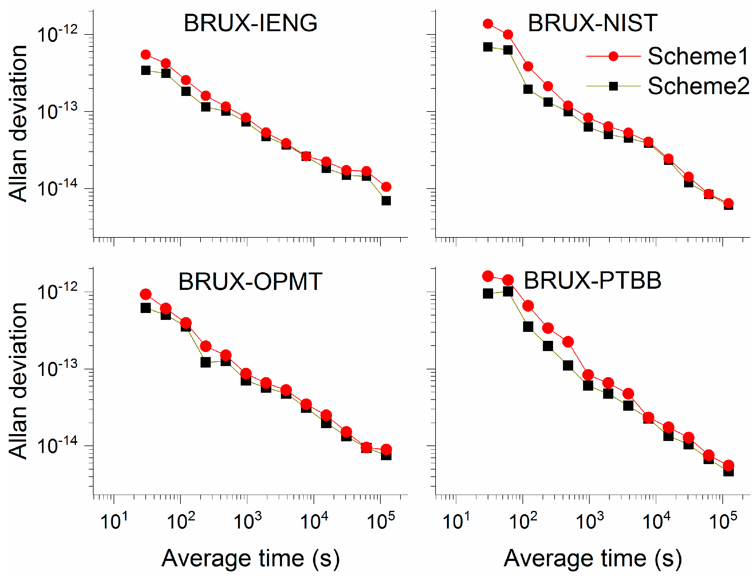
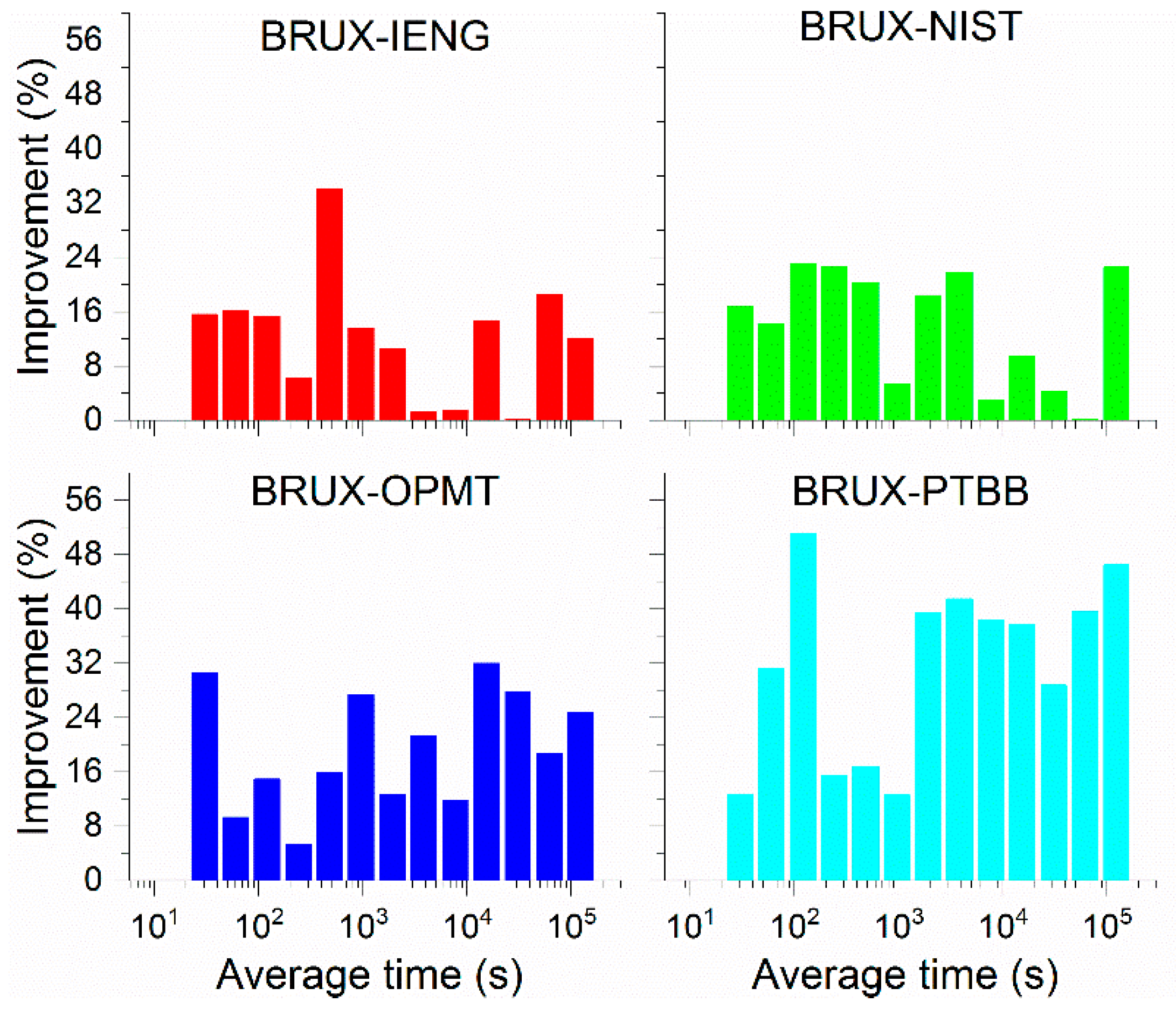
4.1. Results of the Simulation Data Set

In this subsection, the simulation data are utilized to validate how our approach performs when data interruption occurs.

In Figure 5, each panel shows three types of time series of clock offset estimation with a time resolution of 10 min data interruption on BRUX. Other stations perform a similar feature; hence, we will no longer display them in detail. Furthermore, the clock difference in the time series of scheme 1 and scheme 2, with respect to the results of the complete data with the between-epoch constraint model, is displayed in Figure 6 for a data interruption of 10 min. Combining Figure 5 and Figure 6 results in two findings. For one thing, as we noted earlier, the clock offset will re-converge, especially for scheme 1, when the data interruption occurs. Obviously, the results from the complete data show some fluctuation (see Figure 6), as evidenced by the fact that the ambiguity parameters cannot instantaneously yield stable results, although we have constrained 20 consecutive epochs. Additionally, compared with the results from scheme 1, scheme 2 shows no obvious jump when the data interruption occurs. This can be explained by the fact that a prior clock offset is constrained by the prediction results.

For a better quantification, we calculated the RMS of the two schemes using the corresponding time series of the complete data as a reference; the results are presented in

Table 4. RMS of the clock difference between the solutions obtained with two different schemes with respect to the solutions obtained with the complete data when data interruption occurs (ns).

	10 min			30 min			60 min			90 min
	Sch1	Sch2	(%)	Sch1	Sch2	(%)	Sch1	Sch2	(%)	Sch1	Sch2	(%)
BRUX	0.44	0.14	68.64	0.43	0.14	67.99	0.46	0.16	65.22	0.45	0.18	59.93
IENG	0.40	0.11	71.43	0.41	0.17	58.38	0.39	0.18	53.52	0.41	0.22	46.34
NIST	0.40	0.15	61.71	0.40	0.14	64.49	0.39	0.16	60.31	0.44	0.21	51.67
OPMT	0.50	0.19	61.99	0.51	0.18	64.89	0.49	0.20	58.70	0.51	0.20	59.71
PTBB	0.52	0.15	71.22	0.53	0.15	72.06	0.52	0.18	65.38	0.51	0.23	54.10
WAB2	0.36	0.15	58.48	0.37	0.15	58.72	0.36	0.23	36.11	0.37	0.26	30.96

Where sch1 and sch2 represent scheme 1 and scheme 2, respectively, and (%) is the improvement of scheme 2 over scheme 1.

. Note that we have deleted the gross errors before calculating the RMS values. The maximum RMS values for scheme 1 are 0.52 ns for all stations with 10-, 30-, 60-, and 90-min data interruptions, while the corresponding maximum RMS values are 0.19, 0.18, 0.20, 0.23 and 0.26 ns for scheme 2. The improvement percentage of scheme 2 shows that the average RMS values of all stations are significantly reduced, i.e., by 66.03% from 0.43 to 0.14 ns, by 64.91% from 0.44 to 0.15 ns, by 57.47% from 0.43 to 0.18 ns, and by 51.67% from 0.44 to 0.21 ns for 10-, 30-, 60-, and 90-min data interruptions, respectively. This implies that scheme 1 is not as good as our approach. We surmise this may be attributed to two reasons. First, the between-epoch constraint model will reduce the noise of the clock offset. Second, our approach does not produce jumps that may accelerate clock offset convergence.

The Allan deviation (ADEV) is employed to obtain the frequency stability [8,28], which is also utilized to further assess the performance of RT-PPP solutions, using five kinds of precise products. In this contribution, Stable32 software (http://www.wriley.com/) is applied to calculate ADEV. Note that the gross error of all RT-PPP solutions is eliminated before computing ADEV by using Stable32 software (Hamilton Technical Services, Beaufort, SC, USA).

With the different lengths of the missing observations and two scenarios, Figure 7 and Figure 8 demonstrate the effects of the Allan deviation based on six stations. Many similarities can be found from the figures. From 10 to 90 min, regardless of the length of the observation interruption, the results from all the selected stations indicate that scheme 2 is more stable than scheme 1. The magnitude of the improvement at the six stations is very similar. This is because the same random-walk model is constrained by the atomic clock. The general results demonstrate that scheme 2 is more suitable to estimate the receiver clock offset than scheme 1.

The inspection of Figure 9 can reveal more about the improvement of the frequency stability at a specific averaging time. The data indicate that all the involved stations are improved at each averaging time. Furthermore, as the averaging time increases, the improvement percent decreases. Before 10000 s, the improvement extent of the six stations was up to 50% from data interruptions of 10 min to 90 min; some points even improved by 100%. However, after 10000 s, the improvement extent of the six stations fell below 50%; some points being at only 1%. Briefly, compared to scheme 1, scheme 2 works well for short-term stability. The Allan deviation is a common measure of the frequency stability. Although the definition for short-term stability and long-term stability is the same, they reflect different characteristics of the signal stability. Short-term stability mirrors the signal’s fluctuations, and long-term stability represents the signal’s drift as time goes by. The between-epoch constraint model merely lowers the noise of the clock offset time series; however, it cannot change the physical trend of the atomic clock. Hence, there are enough reasons to certify that the random-walk model is an effective approach for improving stability at each averaging time.

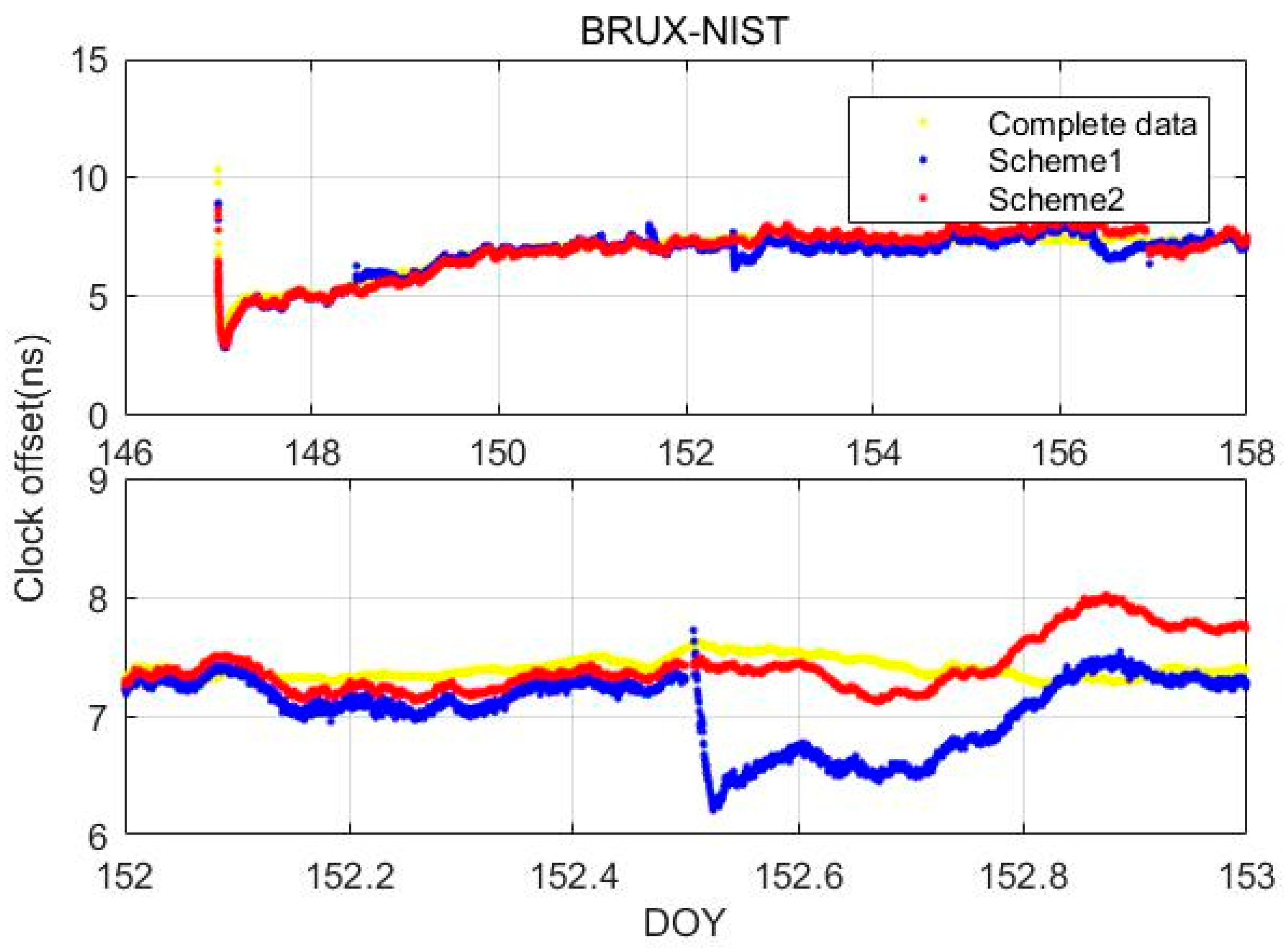
4.2. Results of the Real Data Set

In this subsection, real data are utilized to validate how our approach performs when data interruption occurs. The real-time stream interruption occurs occasionally under unknown conditions. The real-time stream CLK 81 is employed here. The investigation is performed from DOY 147–158, 2018. The monitoring system records the data interruption at some times. The abnormal data are stored to verify the new algorithm. Because the time reference of real-time satellite clocks is not a continuous clock or time scale, the clock solution of a single station is not reliable when evaluating the new model. For this reason, only a link result can be used for the stability evaluation with the purpose of removing the uncertainty of the reference. Four links are calculated with the real data set. One link is demonstrated in below. In the real data section, all the time transfer experiments are obtained with BRUX as the pivot.

Figure 10 and Figure 11 show, first, that the clock difference time series of scheme 2 is smoother than that of scheme 1. Second, the non-convergence caused by the observation interruption occurs in scheme 1, causing the appearance of a system error. It influences the stability of the time link. Third, the tendency of scheme 2 is in accordance with the complete data, i.e., the data show that scheme 2 avoids re-convergence when the data are interrupted. The data show that scheme 2 works well for the real time data and for the simulation data.

Figure 12 and Figure 13 illustrate more about the link stability. All the stations are equipped with an H-maser. The discrepancy in the different types of external frequency standard can be neglected. For the selected four links, the data show that the time series in scheme 2 is more stable than that in scheme 1. The maximum percentage of improvement is greater than 50%, while the minimal percentage of improvement is 5%. In other words, the frequency of stability is boosted at each averaging time, especially in the link BRUX-PTBB, where a distinct enhancement is demonstrated at each averaging time. The maximum percentage is greater than 50% at 100 s. A strong correlation may exist in the adjacent epoch for the PTB’s H-MASER. The application of the between-epoch constraint clock model makes full use of the correlative information to achieve more stable results. Moreover, the data show that the magnitude of the improvement is not correlated to the distance between the stations.

5. Conclusions

The GNSS orbit and clock corrections from the real-time stream transform the real-time or low-latency PPP time transfer into a possible time transfer that has practical significance for timing laboratories. To escape the embarrassment of a receiver clock offset re-convergence caused by a data interruption, in this study, a new algorithm is proposed to resolve the discontinuity induced by the re-convergence. A combination of a between-epoch constraint receiver clock model and an adaptive clock prediction model is added to the ionosphere-free observation equation. A comparison is also made with the results obtained using the white noise model, regardless of the physical design of the atomic clock. All the results calculated from the single station and the links show that the statistical uncertainty with the between-epoch constraint receiver clock model was less than that of the white noise model. The simulation results show that the average RMS values at all the stations are significantly reduced, i.e., by 66.03% from 0.43 to 0.14 ns, by 64.91% from 0.44 to 0.15 ns, by 57.47% from 0.43 to 0.18 ns, and by 51.67% from 0.44 to 0.21 ns for 10-, 30-, 60-, and 90-min data interruptions, respectively. Furthermore, the time series adopted by the new model was more stable than that of a white noise model. The observed detail shows that the improvement magnitude of the stability acquired with the single station is significantly correlated with the averaging time. The between-epoch constraint receiver clock model is more effective for short-term stability than for long-term stability. The extent of the improvement at the six stations was greater than 50% prior to 10000 s, even reaching 100% at the initial averaging time. The data do not show a close correlation between the distance of the two stations and the level of improvement. The frequency stability of the time link is boosted by at least 5% at each averaging time. The results gained from the PPP strategy conducted using the simulation data and the IGS real-time data indicate that the new method can satisfy low-latency time transfer.

References

1. Allan, D.W.; Weiss, M.A. Accurate time and frequency transfer during common-view of a GPS satellite. In Proceedings of the 1980 IEEE Frequency Control Symposium, Philadelphia, PA, USA, 28–30 May 1980; pp. 334–356. [Google Scholar]
2. Petit, G.; Jiang, Z. GPS All in View time transfer for TAI computation. Metrologia 2008, 45, 35–45. [Google Scholar] [CrossRef]
3. Petit, G.; Jiang, Z. Precise Point Positioning for TAI Computation. Int. J. Navig. Obs. 2008, 2008, 1–8. [Google Scholar] [CrossRef] [Green Version]
4. Zumberge, J.F.; Heflin, M.B.; Jefferson, D.C.; Watkins, M.M.; Webb, F.H. Precise point positioning for the efficient and robust analysis of GPS data from large networks. J. Geophys. Res. 1997, 102, 5005–5017. [Google Scholar] [CrossRef] [Green Version]
5. Kouba, J.; Héroux, P. Precise point positioning using IGS orbit and clock products. GPS Solut. 2001, 5, 12–28. [Google Scholar] [CrossRef]
6. Petit, G. The TAIPPP pilot experiment. In Frequency Control Symposium, 2009 Joint with the 22nd European Frequency and Time forum. IEEE Int. 2009, 1–2, 116–119. [Google Scholar]
7. Petit, G.; Kanj, A.; Loyer, S.; Delporte, J.; Mercier, F.; Perosanz, F. 1 × 10⁻¹⁶ frequency transfer by GPS PPP with integer ambiguity resolution. Metrologia 2015, 52, 301–309. [Google Scholar] [CrossRef]
8. Ge, Y.; Qin, W.; Cao, X.; Zhou, F.; Wang, S.; Yang, X. Consideration of GLONASS Inter-Frequency Code Biases in Precise Point Positioning (PPP) International Time Transfer. Appl. Sci. 2018, 8, 1254. [Google Scholar] [CrossRef]
9. Ge, Y.; Yang, X.; Qin, W.; Su, H.; Wu, M.; Wang, Y.; Wang, S. Time Transfer Analysis of GPS- and BDS-Precise Point Positioning Based on iGMAS Products. China Satell. Navig. Conf. 2018, 497, 519–530. [Google Scholar]
10. Tu, R.; Zhang, P.; Zhang, R.; Liu, J.; Lu, X. Approach for GPS precise time transfer using an augmentation information and zero-differenced PPP model. IET Radar Sonar Navig. 2018, 12, 801–806. [Google Scholar] [CrossRef]
11. Zhang, P.; Tu, R.; Zhang, R.; Gao, Y.; Cai, H. Combining GPS, BeiDou, and Galileo Satellite Systems for Time and Frequency Transfer Based on Carrier Phase Observations. Remote Sens. 2018, 10, 324. [Google Scholar] [CrossRef]
12. Hadas, T.; Bosy, J. IGS RTS precise orbits and clocks verification and quality degradation over time. GPS Solut. 2014, 19, 93–105. [Google Scholar] [CrossRef] [Green Version]
13. Li, X.; Ge, M.; Douša, J.; Wickert, J. Real-time precise point positioning regional augmentation for large GPS reference networks. GPS Solut. 2013, 18, 61–71. [Google Scholar] [CrossRef] [Green Version]
14. Laurichesse, D.; Mercier, F.; Berthias, J.P. Real time precise GPS constellation orbits and clocks estimation using zero-difference integer ambiguity fixing. In Proceedings of the 2009 International Technical Meeting of the Institute of Navigation, Anaheim, CA, USA, 26–28 January 2009; pp. 664–672. [Google Scholar]
15. Zhang, P.; Tu, R.; Gao, Y.; Liu, N.; Zhang, R. Improving Galileo’s Carrier-Phase Time Transfer Based on Prior Constraint Information. J. Navig. 2019, 72, 121–139. [Google Scholar] [CrossRef]
16. Li, G.; Lin, Y.; Shi, F.; Liu, J.; Yang, Y.; Shi, J. Using IGS RTS Products for Real-Time Subnanosecond Level Time Transfer. China Satell. Navig. Conf. 2018, 497, 505–518. [Google Scholar]
17. Defraigne, P.; Aerts, W.; Pottiaux, E. Monitoring of UTC(k)’s using PPP and IGS real-time products. GPS Solut. 2014, 19, 165–172. [Google Scholar] [CrossRef]
18. Hauschild, A.; Montenbruck, O. Kalman-filter-based GPS clock estimation for near real-time positioning. GPS Solut. 2008, 13, 173–182. [Google Scholar] [CrossRef]
19. Boehm, J.; Niell, A.; Tregoning, P.; Schuh, H. Global Mapping Function (GMF): A new empirical mapping function based on numerical weather model data. Geophys. Res. Lett. 2006, 33. [Google Scholar] [CrossRef] [Green Version]
20. Zhou, F.; Dong, D.; Ge, M.; Li, P.; Wickert, J.; Schuh, H. Simultaneous estimation of GLONASS pseudorange inter-frequency biases in precise point positioning using undifferenced and uncombined observations. GPS Solut. 2017, 22, 19. [Google Scholar] [CrossRef]
21. Wu, J.T.; Wu, S.C.; Hajj, G.A.; Bertiger, W.I.; Lichten, S.M. Effects of antenna orienation on GPS carrier phase. Manuscr. Geod. 1992, 18, 91–98. [Google Scholar]
22. Montenbruck, O.; Schmid, R.; Mercier, F.; Steigenberger, P.; Noll, C.; Fatkulin, R.; Kogure, S.; Ganeshan, A.S. GNSS satellite geometry and attitude models. Adv. Space Res. 2015, 56, 1015–1029. [Google Scholar] [CrossRef] [Green Version]
23. Hutsell, S. Relating the Hadamard Variance to MCS Kalman Filter Clock Estimation. In Proceedings of the 27th Annual PTTI Systems Applications Meeting, San Diego, CA, USA, 29 November–1 December 1995; pp. 291–301. [Google Scholar]
24. Wang, K.; Rothacher, M. Stochastic modeling of high-stability ground clocks in GPS analysis. J. Geod. 2013, 87, 427–437. [Google Scholar] [CrossRef]
25. Kazmierski, K.; Sośnica, K.; Hadas, T. Quality assessment of multi-GNSS orbits and clocks for real-time precise point positioning. GPS Solut. 2017, 22, 11. [Google Scholar] [CrossRef]
26. Wang, Z.; Li, Z.; Wang, L.; Wang, X.; Yuan, H. Assessment of Multiple GNSS Real-Time SSR Products from Different Analysis Centers. ISPRS Int. J. Geo-Inf. 2018, 7, 85. [Google Scholar] [CrossRef]
27. Zhang, L.; Yang, H.; Gao, Y.; Yao, Y.; Xu, C. Evaluation and analysis of real-time precise orbits and clocks products from different IGS analysis centers. Adv. Space Res. 2018, 61, 2942–2954. [Google Scholar] [CrossRef]
28. Guang, W.; Dong, S.; Wu, W.; Zhang, J.; Yuan, H.; Zhang, S. Progress of BeiDou time transfer at NTSC. Metrologia 2018, 55, 175–187. [Google Scholar] [CrossRef]
Figure 1. Diagram of the adaptive prediction clock model.
Applsci 09 01405 g001
Figure 2. Diagram of the RT-PPP (real-time PPP) time and frequency transfer using the clock model.
Applsci 09 01405 g002
Figure 3. Clock offset time series using different models (red-5 ns).
Applsci 09 01405 g003
Figure 4. Prediction error of the adaptive clock prediction model at station BRUX at 10, 30, 60 and 90 min.
Applsci 09 01405 g004
Figure 5. Clock offset time series for scheme 1 (blue) and scheme 2 (red) when a data interruption of 10 min occurs; the yellow colour represents the solutions of the complete data using the between-epoch constraint model; the bottom figure is a partial amplification of the top figure.
Applsci 09 01405 g005
Figure 6. Clock difference time series using scheme 1 (blue) and scheme 2 (red) with respect to the results of the complete data using the between-epoch constraint model when a data interruption of 10 min occurs; the bottom figure is a partial amplification of the top figure.
Applsci 09 01405 g006
Figure 7. Allan deviation of scheme 1 (blue) and scheme 2 (red) at six stations for observation interruptions of 10 and 30 min.
Applsci 09 01405 g007
Figure 8. Allan deviation of scheme 1 (blue) and scheme 2 (red) at six stations for observation interruptions of 60 and 90 min.
Applsci 09 01405 g008
Figure 9. Improvement of the frequency stability (percent) of scheme 2 compared to scheme 1.
Applsci 09 01405 g009
Figure 10. Clock offset time series of scheme 1 (blue) and scheme 2 (red); the yellow colour represents the solutions of the complete data with the between-epoch constraint model; the bottom figure is a partial amplification of the top figure.
Applsci 09 01405 g010
Figure 11. Clock difference time series of scheme 1 (blue) and scheme 2 (red) with respect to the results of the complete data with the between-epoch constraint model when 10 min of data interruption occurs; the bottom figure is a partial amplification of the top figure.
Applsci 09 01405 g011
Figure 12. Allan deviation of scheme 1 (blue) and scheme 2 (red) on four links.
Applsci 09 01405 g012
Figure 13. Percent of improvement of the frequency stability of scheme 2, compared to scheme 1.
Applsci 09 01405 g013