Featured Application
A complete framework of on-orbit polarization calibration for the multichannel polarimetric camera is presented. Its advantage is that it shares the same calibration assembly with the radiometric calibration and doesn’t need the extra polarized light source or large polarizer. This polarization calibration framework for the multichannel polarimetric camera is useful for the subsequent polarimetric camera.
Abstract
In this paper, a new on-orbit polarization calibration method for the multichannel polarimetric camera is presented. A polarization calibration model for the polarimetric camera is proposed by taking analysis of the polarization radiation transmission process. In order to get the polarization parameters in the calibration model, an on-orbit measurement scheme is reported, which uses a solar diffuser and a built-in rotatable linear analyzer. The advantages of this scheme are sharing the same calibration assembly with the radiometric calibration and acquiring sufficient polarization accuracy. The influence of the diffuser for the measurement is analyzed. By using a verification experiment, the proposed method can achieve on-orbit polarization calibration. The experimental results show that the relative deviation for the measured degree of linear polarization is 0.8% at 670 nm, which provides a foundation for the accurate application of polarimetric imaging detection.
1. Introduction
The polarimetric remote sensing camera is an optical detection system, which is designed for the polarimetric imaging of the target. It can obtain the degree and the angle of linear polarization, not just the radiance. The polarization information has a multitude of applications in many fields, including agriculture, military reconnaissance, meteorological environment monitoring and other fields [1,2,3]. At present, most of the detection instruments used for polarization remote sensing are the first-generation polarization detection systems. The types of these systems include the division-of-time (DoT), the division-of-amplitude (DoAM), the division-of-aperture (DoAP) and the division-of-focal plane (DoFP) [4,5]. However, each type has its own weakness, such as the calibration problem of the types of DoAM and DoAP [6], the imaging field of view (IFOV) errors of the type of DoFP [7,8]. However, the polarizing effects caused by the polarimetric camera itself will affect the accuracy of polarization detection. In addition, the polarizing effects are changed by the optical structure, material and so on. For the above reasons, the polarization characteristics of polarized cameras operating in space will be different from those in laboratory calibration. Therefore, the instrument should make the on-orbit polarization calibration at regular intervals to ensure that the detection accuracy is not reduced. This paper intends to provide an on-orbit polarization calibration method for a multichannel polarimetric camera with DoAM. This method has many technological advantages, such as a high maturity and stability, wide spectral range, and large field of view.
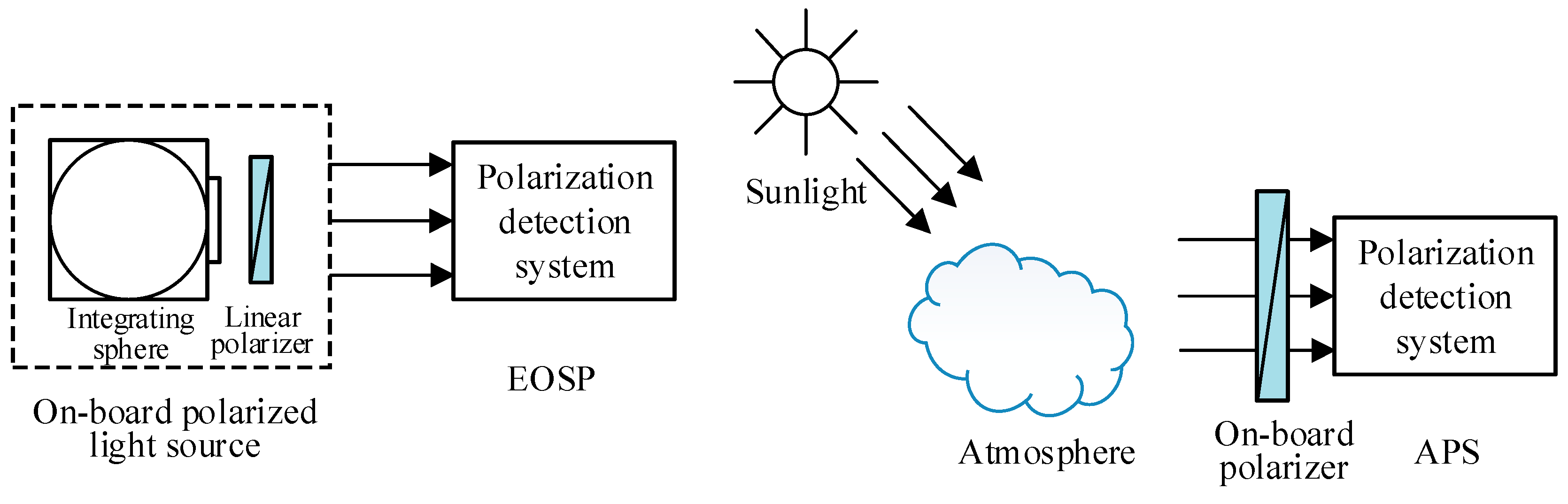
At present, the commonly used on-orbit calibration methods include the scene calibration, the on-board polarized light source method and the spaceborne linear polarization method. The Polarization and Directionality of the Earth’s Reflectance (POLDER) and the Directional Polarized Camera (DPC) has adopted the scene calibration [9,10]. When the polarimetric camera observes the atmosphere in a specific angle, the light reflected by the atmosphere is close to the unpolarized light. The camera uses this source as a calibration source for polarization calibration. However, it is hard to meet the requirement of obtaining unpolarized light when observing the atmosphere in reality. Even if the scene calibration method is a simple and easy to operate method, the calibration accuracy is low. The on-board polarized light source method (see Figure 3) has the highest precision, which is used by the Earth Observing Scanning Polarimeter (EOSP) [11]. The advantage of this method is that the polarization calibration can be taken in real time. However, one of the problems of this method is that the system lifetime is restricted by the polarized light source. The other problem is that the volume and power cannot meet the satellite constrains. The spaceborne linear polarization method which has been adopted in Aerosol Polarimetry Sensor (APS) can solve the above problems [12]. When the polarimetric camera observes the atmosphere in a specific angle, the on-board polarizer will create polarized light which can be used for the calibration. The accuracy is high enough, and the lifetime of the on-board polarizer is as long as the satellite. The main problem of this method is that the polarizer should cover all fields of view for the optical system, which means that the polarizing plate will be very large. All of the methods above have some inherent problems. Therefore, it is necessary to study a new on-orbit polarization calibration method with high accuracy, small volume and reliable performance.
In this paper, we propose a new on-orbit polarization calibration method, which is called the on-orbit rotating analyzer polarization calibration method. The calibration source is the unpolarized light created by an on-board solar diffuser which can be shared with the on-orbit radiometric calibration. A built-in rotatable linear polarizer (herein, called the linear analyzer) is used to analyze the polarizing effects of the camera. Additionally, the built-in linear analyzer can be very small, as it is placed after the optical system. Here, we used a micro precision rotation stage to control the linear analyzer to rotate precisely. When the polarimetric camera is taking on-orbit solar radiometric calibration, the linear analyzer rotates continuously. The Stokes parameters were calculated by the received radiation intensity. A special model is established for polarization calibration of the polarimetric camera. The proposed method can meet the need of on-orbit polarization calibration with a higher accuracy.
This paper is organized as follows. In Section 2, the main polarization parameters of the camera are analyzed, based on the principle of a multichannel polarimetric camera. In Section 3, the new polarization calibration method is proposed, including the calibration model, on-orbit measurement scheme and the factors acting on the calibration accuracy. Section 4 describes a verification experiment which is conducted to verify the accuracy of the polarization calibration method that this paper proposed. In Section 5, we summarize and conclude the paper.
2. The Multichannel Polarimetric Camera and Main Polarization Elements
2.1. The Multichannel Polarimetric Camera
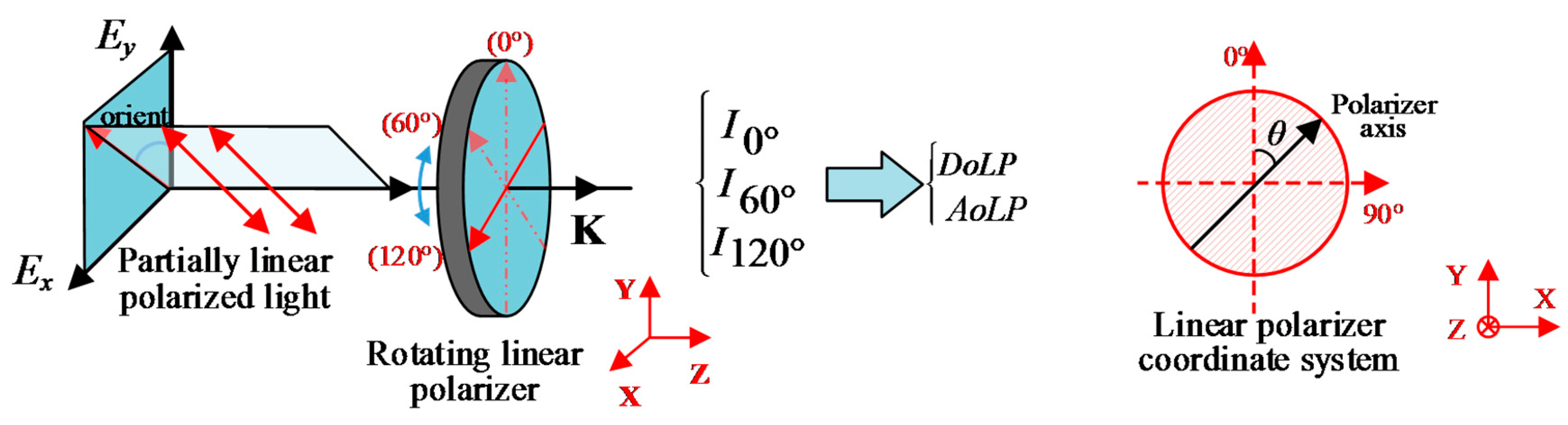
In the field of remote sensing, it has great significance in measuring the polarization information of the target, especially the information of degree of linear polarization (DoLP). In this paper, the DoLP describes the proportion of the linear polarized light among all the polarization states of light (unpolarized, linear polarized, circularly polarized and elliptically polarized light), and the angle of linear polarization (AoLP) describes the oscillation direction of the linear polarized light [13]. As we know, the polarization information (DoLP, AoLP) of the light can be measured by using a rotating linear analyzer [14]. The polarization information can be calculated by using Equation (1) with the radiance at three specific angles (I0°, I60°, and I120°) of the analyzer.
where I, Q, U denote the Stokes parameters. The measurement method for the polarization information on partially linear polarized light is shown in Figure 1. A linearly polarized parallel light of known polarization direction may be employed, and the non-ideal linear polarizer is incident. By rotating the non-ideal linear polarizer, the light intensity at different analyzer angles is obtained, and the parameters of the non-ideal linear polarizer are obtained by fitting.
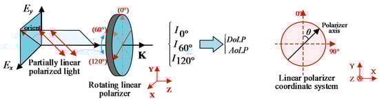
Figure 1.
Measurement method for the polarization information on partially linear polarized light.
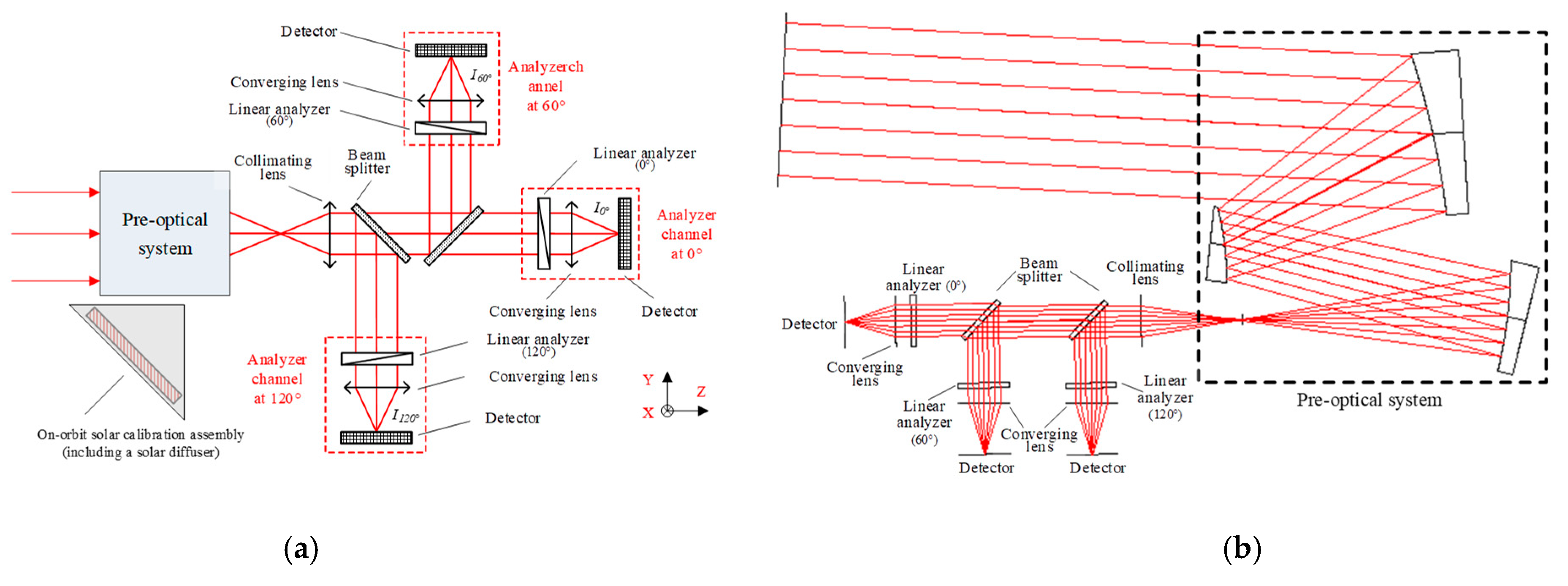
Since the method above needs to rotate the analyzer three times, the measurement cannot be updated in real time. Therefore, we propose a multichannel polarization camera that enables real-time shooting. Three fixed analyzers with three polarization axis angles, which are 0°, 60°, and 120°, are proposed to measure the polarization information simultaneously. The schematic of the multichannel polarimetric camera is shown in Figure 2a. The optical design model of the multichannel polarimetric camera is illustrated in Figure 2b. The image of the target is caught by the pre-optical system. The collimating lens transforms the imaging light into parallel light. The parallel light is separated into three channels by two beam splitters located in the rear of the collimating lens. The polarization state of the imaging light can be detected by three polarization analyzer channels, which are composed of three separate linear analyzers. In each analyzer channel, the parallel light is focused by a converging lens and received by a detector. The three polarizer axis angles of the linear analyzers are 0°, 60°, and 120°, respectively.
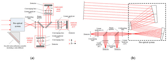
Figure 2.
(a) Schematic of the multichannel polarimetric camera and (b) optical design model of the multichannel polarimetric camera. The incident light is represented by the red solid lines. The three channels (analyzer channels at 0°, 60°, and 120°) are indicated by the red dotted boxes.
2.2. Main Polarization Parameters of the Polarimetric Camera
Comparing with Figure 1 and Figure 2, we can know that the polarimetric camera is much more complex than the method of using a rotating linear polarizer. According to the Fresnel formula, when the light is reflected or refracted on the optical surface, the polarization state of the reflected or refracted light is changed because of the polarizing effects. Therefore, it is necessary to consider the polarizing effects of the optical elements in the polarimetric camera.
However, due to the restriction of space and power on the satellite, it is unpractical to take the on-orbit polarization calibration for every optical element. A realizable way is proposed to analyze the polarizing effects of the polarimetric camera and take calibration to the main polarization elements, whose polarizing effects are more notable [15].
As we know, the polarizing effects are related to the optical structure, material, wavelength, aperture and coating [13]. In this multichannel polarimetric camera, the collimating lens, the beam splitters and the converging lens can be designed and optimized into approximately unpolarized elements, because their diameters and aperture angles are small. [16] The degree of polarization of the optics decreases as the angle of view decreases. At a 670 nm channel, an optical component with a field of view of 0.3 rad has a degree of polarization lower than 0.01. That means we should consider the polarizing effects of the pre-optical system and linear analyzers.
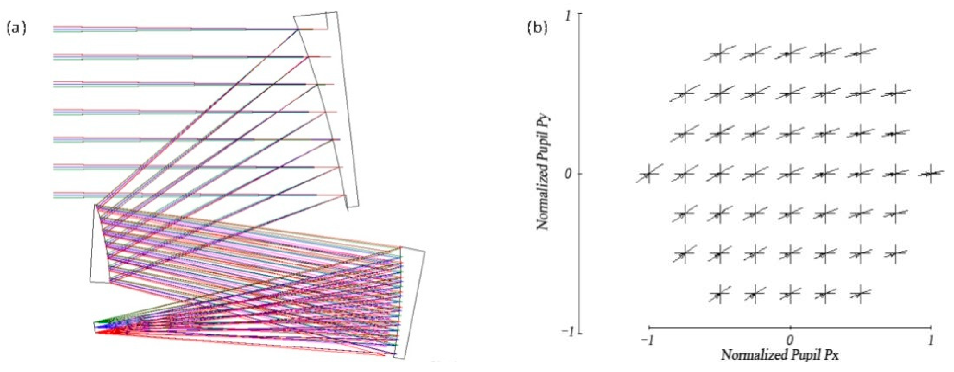
The polarizing effects cannot be eliminated by optimization design. The pre-optical system of the polarimetric camera is an off-axis three-mirror reflective configuration, which is commonly used for space remote sensing detection. The mirrors are made of aluminum and the effect of the coating for polarization can be ignored which has low phase retardance [17]. For a filmless optical system, the polarization characteristics are determined by the incident angle, exit angle, incident wavelength, and refractive index of the interface, which can be calculated by the Fresnel formula. The entrance pupil diameter is 150 mm and the focal length is 500 mm. The polarizing effects of the optical system at the exit pupil are analyzed by means of the POLDSP.SEQ macro in CODE V [18]. The design model of the optical system and the analysis result are shown in Figure 3. The polarizing effects is expressed by the diattenuation ε1 and the phase retardance θ [13], where the diattenuation is defined by ε1 = (Rs − Rp)/(Rs + Rp), in which Rs and Rp represent the maximum and minimum intensity reflectance, respectively [14]. When the incent light is unpolarized light, the polarization state at the exit pupil can also describe the polarizing effects, which contains partially linear polarized light, partially circular polarized light, and partially elliptical polarized light.

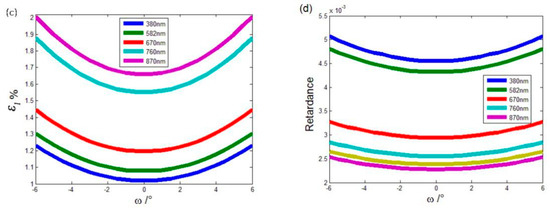
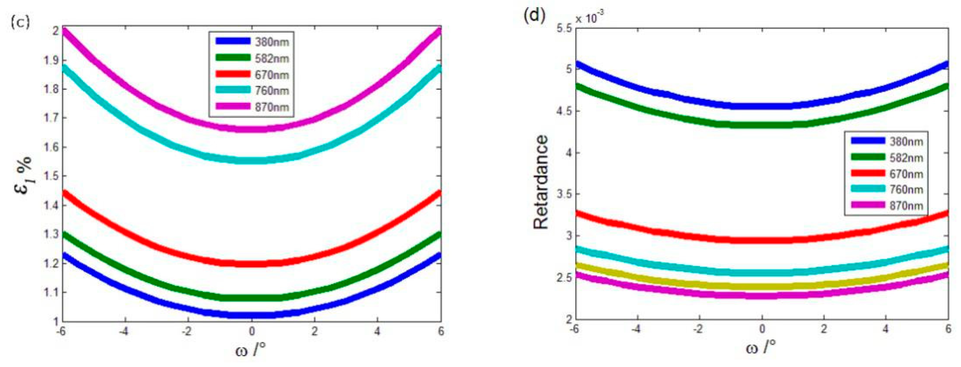
Figure 3.
(a) Design model of the pre-optical system; (b) analysis result of polarization state at 870 nm; (c) analysis result of diattenuation; (d) analysis result of phase retardance. The field of view of the optical system is 2ω = 12°.
Figure 3b shows that the polarization state of the exit light is a partially linear polarized light. We can see from Figure 3c,d that the diattenuation ε1 and the retardance are changed according to the field of view and the wavelength. The parameters rise as the increase of the field of view. The material or the coating of the mirrors decides their changes as the wavelength. For the material of aluminum, the diattenuation ε1 at 870 nm is larger than the other wavelength. On the contrary, the retardance at 870 nm is smaller than the other wavelength. From the figures above, we can see that the maximum polarization degree ε1 for this system is up to 2%, and the biggest phase retardance for this system is less than 0.005°. In this case, the influence of the diattenuation ε1 for this system cannot be ignored, and the phase retardance for this system can be ignored, which can be indicated by Figure 3.
The performance of a linear analyzer is described by the extinction ratio E, which is defined by E = Ty/Tx, where Tx and Ty represent the maximum and minimum transmittance of the two orthogonal directions, respectively [19]. Here, the extinction ratio E can represent the diattenuation of the linear analyzer, because they can be converted into each other [13]. For an ideal analyzer, the extinction ratio E is quite close to zero. But the extinction ratio of this analyzer (Wire Grid Polarizers on Glass Substrates, WP25M-UB, THORLABS) is not high enough, because it is usually made up of a wire grid for a large acceptance angle. For a common wire grid analyzer, it isn’t an ideal analyzer as the extinction ratio at visual band is E = 1/200. When we are only concerned about the analyzer, the relative deviation δ(E) of polarization detection with reference to an ideal analyzer is calculated as [20].
When the extinction ratio is E = 1/200, the relative deviation is δ(E) = 1%, which also should be calibrated for high accuracy.
The polarizer axis angles of the linear analyzers can also influence the accuracy of the polarimetric camera. The accuracy of polarization axis inclination of linear analyzer affects the precision of the polarization camera [21]. It can be calibrated by a computer-aided method.
We can see from the above analysis that the main polarization parameters of the camera, which need to be calibrated, are the diattenuation of the pre-optical system (ε1) and the wire grid analyzer (E). As there is only an on-orbit solar calibration assembly on this satellite for calibration, the polarization calibration method should be newly designed. A new method of on-orbit polarization calibration should be presented to improve the accuracy of the polarimetric camera, which needs no extra device except for the solar calibration assembly.
3. On-Orbit Rotating Analyzer Polarization Calibration Method for the Multichannel Polarimetric Camera
In this section, we present a novel polarization calibration method. The main purpose is to complete the calibration using the solar calibration assembly. At a 670 nm channel, the instrument measurement accuracy can reach 0.8% after calibration by this method.
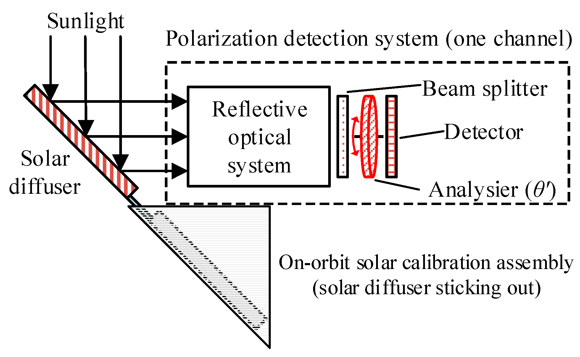
The on-orbit polarization calibration assembly for the EOSP and the APS is shown in Figure 4.
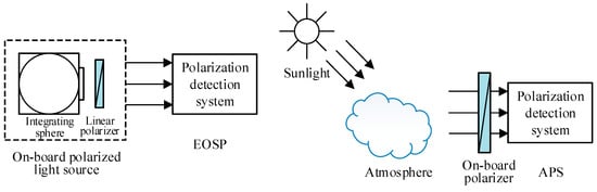
Figure 4.
The on-orbit polarization calibration assembly for the Earth Observing Scanning Polarimeter (EOSP) (left) and the Aerosol Polarimetry Sensor (APS) (right).
We can see from Figure 4 that the main idea of the calibration for the EOSP and the APS is to create polarized light at the entrance pupil of the camera. On the satellite, it’s hard to have sufficient space and power for the on-board polarized light source, when we imitate the calibration method of EOSP. As the diameter of the polarizer should cover all the entrance pupil of the camera, it’s hard to produce a polarizer with such a large diameter (at least 150 mm), if imitating the calibration method of the APS. As the on-board solar diffuser (see Figure 2) is used for on-orbit radiometric calibration in the satellite, it’s quite suitable for polarization calibration. Unlike the method of EOSP and APS, the calibration light of this method is unpolarized light rather than linear polarized light. The polarizing effects of the camera are analyzed by a rotatable analyzer, which is adapted from the built-in fixed linear analyzer. A new calibration model and measurement scheme are proposed.
3.1. On-Orbit Rotary Analyzer Polarization Calibration Model Based on Polarization Optics Theory
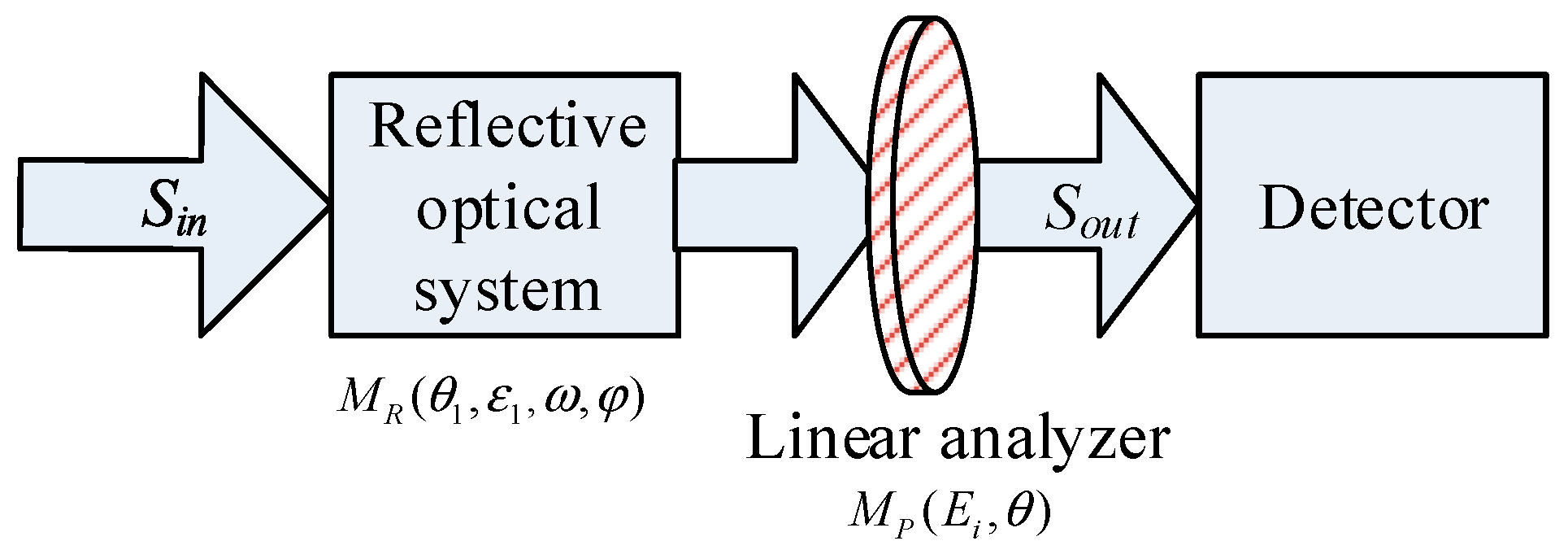
The polarization parameters of the polarizing effects in the optical system are the diattenuation ε1 and its angle of linear polarization θ1. According to the polarization optics theory [19], if all of the depolarization, phase retardance and circular polarized component are ignored, the Mueller matrices [13] for the reflective optical system can be given by
where A (θ1) is the rotation matrices [21]. Here we use ε1 to replace Rs and Rp. The Mueller matrices of the optical system can be rewritten as
where (ω, φ) represents the fields of view (or pixels). Each pixel owns independent Mueller matrices MR (θ1, ε1, ω, φ) as the polarizing effects change as field of view.
For the linear analyzer of the polarimetric camera, the extinction ratio of each polarization analyzer channel is Ei (0 ≤ Ei < 1, for an ideal analyzer, Ei = 0), where i = 1, 2, 3 represents the three polarization analyzer channels. The polarizer axis angle of the linear analyzer is θ, which has been depicted in Figure 1. Its Mueller matrices are given by [19]
As the collimating lens, the beam splitters and converging lens are designed and optimized into approximately unpolarized elements. The polarizing effects can be ignored when their total transmittance in each polarization analyzer channel is Ti (I = 1, 2, 3).
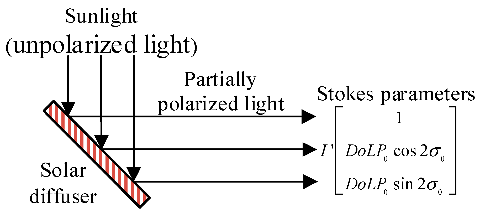
According to the polarization optics theory, when the Stokes vector of the incent light is , the Stokes vector of the light received by the detector is . The schematic of polarization radiation transmission is shown in Figure 5.
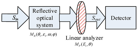
Figure 5.
Schematic of polarization radiation transmission of each analyzer channel.
Tsys(i) is used to describe the polarization radiation transmission factor of each polarization analyzer channel, which is defined by TiTx(Rs + Rp) = Tsys(i). The polarization radiation transmission factors of each channel are different because the transmittances of the beam splitter, the converging lens and the linear analyzer in each channel are different. However, the factors will become the same value after the radiometric calibration, and they can be signed as Tsys. The polarization radiation transmission model of the polarimetric camera can be expressed as
The radiance intensity of the received light is
where the polarizer axis angles θ of each channel are 0°, 60°, and 120°. Therefore, three equations can be created, which include the Stokes vector of the incent light [I, Q, U]. The Stokes vector of the incent light [I, Q, U] can be obtained by solving the Equations (5)–(7). The degree of polarization DoLP and the orient of polarization σorient of the target can be calculated. To simplify the result, the terms are ignored that include the power exponent of the extinction ratio, as the extinction ratio is estimated to be 1/200. The simplified result is
Equations (8)–(12) are the polarization calibration models of the polarimetric camera after the radiometric calibration. The included polarization parameters are the diattenuation ε1 of the optical system, its angle of linear polarization θ1 and the extinction ratio Ei of the linear analyzers. When the polarization parameters are given, the polarizing effects of the polarimetric camera can be calibrated by using this model. In this work, the accuracy of the polarization calibration mainly depended on the accuracy of the polarization parameters, as the accuracy of the radiometric calibration is high enough using an on-board solar diffuser. Actually, the solar radiation has some degree of polarization, which is called the second solar spectrum. The main cause of the second solar spectrum is the uneven distribution of atoms at each sub-level due to the asymmetric radiation field, which is then caused by the large angle scattering of the sun’s edge. The center-to-limb variation (CLV) obtained from the ZIMPOL I polarimeter system shows that the peak Stokes Q/I is very small and this polarization effect is discontinuous in the spectrum [22]. This has less effect on the calibration accuracy of polarized cameras. Therefore, solar radiation can be regarded as an ideal unpolarized light.
3.2. New Measurement Scheme for Polarization Parameters
When the polarimetric camera is taken by the on-orbit polarization calibration, the sunlight is reflected into the camera by the on-board solar diffuser. The radiance intensity received by the detectors can be saved, when the built-in rotatable linear analyzer rotates at every step. The polarization parameters can be obtained by analyzing the change of radiance intensity. This situation is shown schematically in Figure 6.
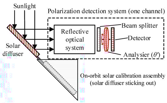
Figure 6.
Schematic of on-orbit polarization calibration.
When the solar diffuser is an ideal Lambertian source, the incent light is unpolarized light. The Stokes vector is , where I’ represents the radiance intensity of the unpolarized light. The polarizer axis angle of the linear analyzer changes from 0° to 360°, which is represented by θ’. The received light of each channel is , which can be rewritten as
The received radiance intensity is
We can see from Equation (13) that the change of the received radiance intensity is an approximate cosine curve. The relationship between the response of the detector and the polarizer axis angle θ’ is as Equation (14), when the polarimetric camera has been taken radiometric calibration. The polarization parameters, the diattenuation ε1, its angle of linear polarization θ1 and the extinction ratio Ei, can be obtained, by taking the least-squares fitting to the response data.
The proposed method of on-orbit polarization calibration not only takes full advantage of the on-board solar diffuser, but also doesn’t need an extra complex polarizer. What it needs is only a micro precision rotation. The calibration accuracy of the method is restricted to the performance of the solar diffuser, and a high control accuracy of the microrotation is required.
3.3. Polarizing Effects of the Solar Diffuser
There are numerous micro-surfaces on the solar diffuser. Ideally, the sunlight is reflected quite diffusely, and the reflected light is unpolarized light. However, the solar diffuser is not an ideal Lambertian source, especially in the case of the aluminium solar diffuser. The aluminium solar diffuser is often used for space remote sensing detection, as its high stability and low cost.
There are some polarizing effects for the aluminium solar diffuser. When the incent light is unpolarized light, the light reflected from the solar diffuser is partially polarized light. According to the Poincare sphere [21], the Stokes parameters of the reflected light can be described by , where DoLP0 represents the polarization degree of the light reflected from the solar diffuser and σ0 represents the polarization angle of the light.
The Stokes parameters of light received by each channel is , and its radiance intensity can be calculated as
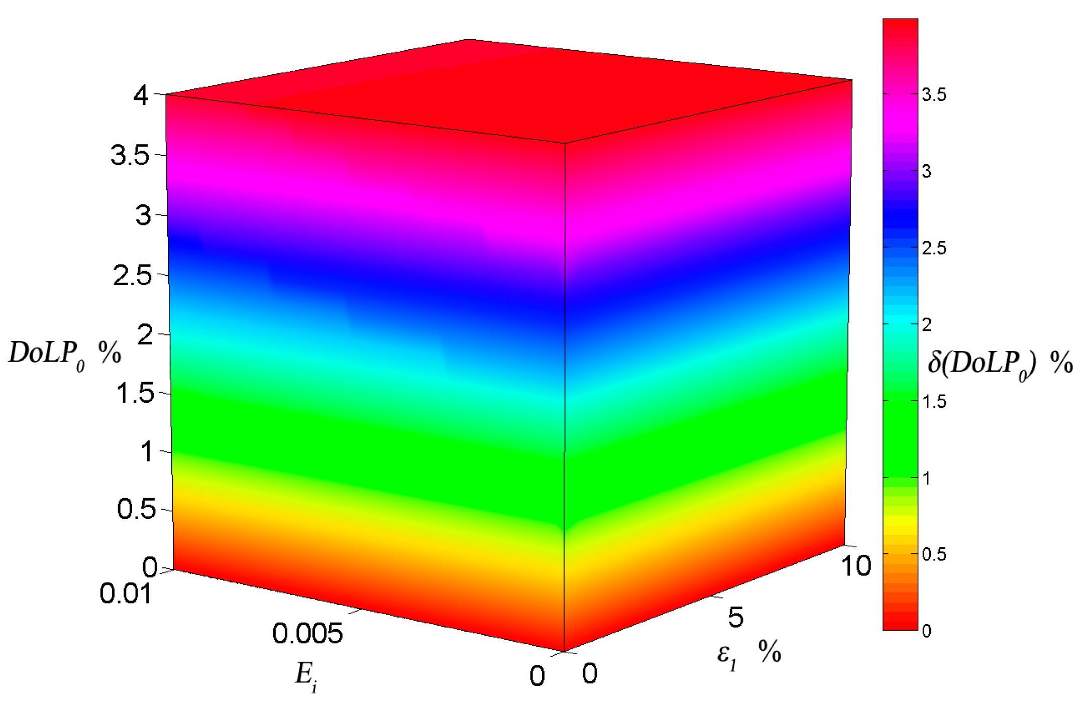
We can analyze the relative deviation of the radiance intensity between an ideal Lambertian source and an actual aluminium solar diffuser from Equation (15). In the development process of this instrument, the physical production process has been optimized by physical grinding and chemical etching. However, there is still no guarantee that the roughness is consistent with the ideal Lambertian body, which leads to the polarization effect. Here, we assume the angle of linear polarization of the diattenuation for the optical system as θ1 = 30°, the polarization angle of the solar diffuser as σ0 = 60°, the polarizer axis angle of the linear analyzer as θ’ = 20°, the range of the extinction ratio as Ei = 0–1/100, the range of the diattenuation of the optical system as ε1 = 0–10%, and the range of the polarization degree of the solar diffuser as DoLP0 = 0–4%. The analysis result of the relative deviation δ(DoLP0) is shown in Figure 7.

Figure 7.
Schematic of the reflection on the solar diffuser.
We can see from Figure 8 that the relative deviation δ(DoLP0) rises as the increase of the polarization degree of the solar diffuser DoLP0. When the polarization degree of the solar diffuser DoLP0 is small (less than the restriction of the accuracy of the calibration), we can use Equation (10) for polarization calibration. Otherwise, we should use Equation (11) for polarization calibration.
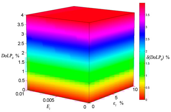
Figure 8.
Analysis result of the relative deviation of the radiance intensity between an ideal Lambertian source and an actual aluminium solar diffuser. We can see that the biggest relative deviation is 4%, when the polarization degree of the solar diffuser DoLP0 changes from 0 to 4%. The polarization degree of the solar diffuser should be as low as possible for on-orbit polarization calibration.
4. Experimental Verification
4.1. Measurement for Polarization Parameters
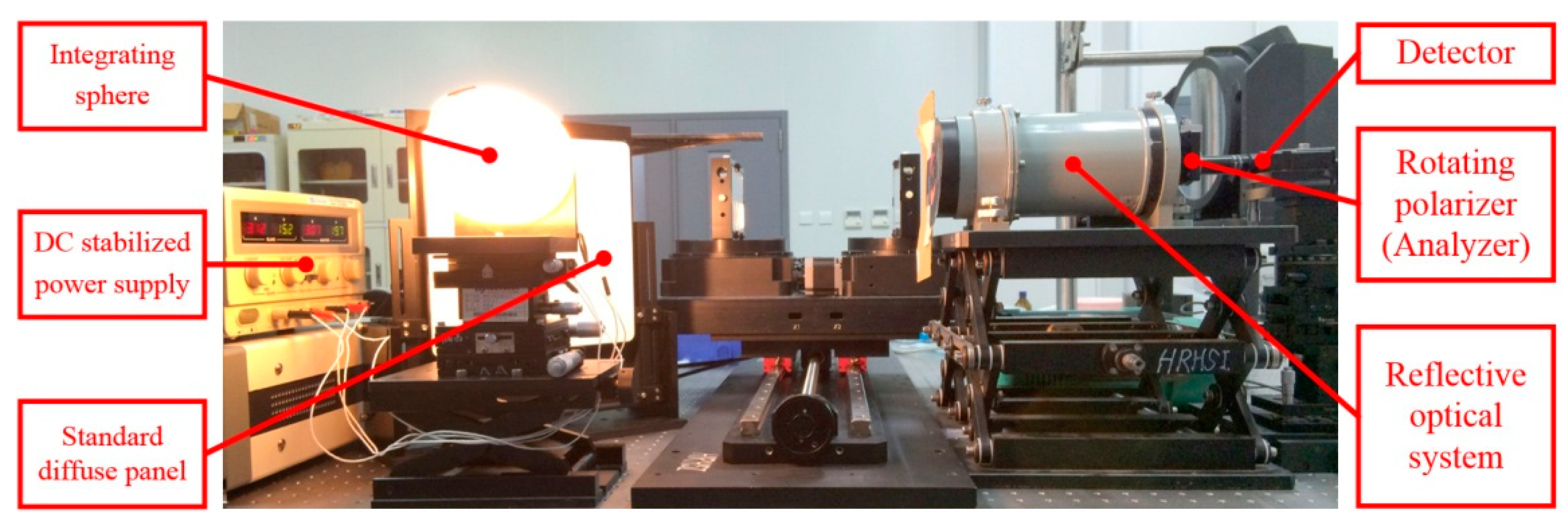
In the verification experiment, the off-axis sub-aperture of a coaxial reflecting optical system was used to simulate the off-axis reflecting optical system of the polarimetric camera. There were a rotating linear analyzer and an ASD detector (single pixel) [23] on the back focal plane. The native polarization sensitivity of the ASD spectrometer has been researched and calibrated [24]. Thereby, an off-axis reflection polarization detection system was simulated. A standard diffuse panel of the Labsphere company is placed between an integrating sphere light source and the simulated polarization detection system for simulating the on-orbit polarization calibration. The linear analyzer was precisely rotated with 10° steps from 0° to 340° by a Newport rotation stage. The measurement system is shown in Figure 9.
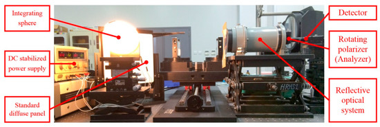
Figure 9.
Photograph of the setup of the measurement system for polarization parameters.
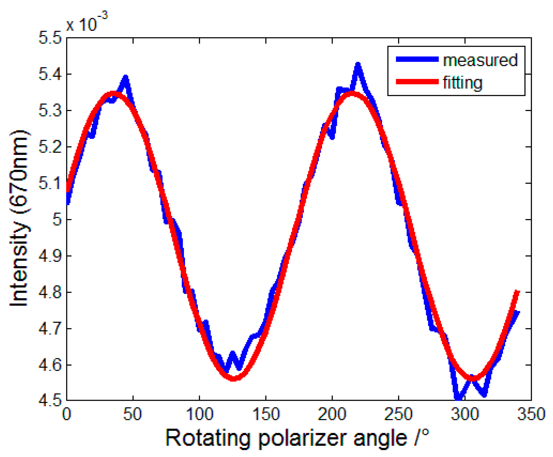
The experimental data and fitting curve are shown in Figure 10.
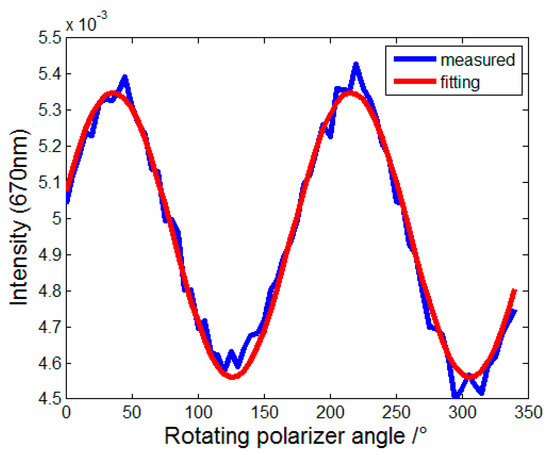
Figure 10.
Experimental data and the fitting curve for the polarization parameters.
The fitting results show that the polarization parameters (670 nm) of the simulated polarimetric camera are obtained: the extinction ratio E = 1/200, the diattenuation of the optical system ε1=7.97% and its angle of linear polarization θ1 = 36°.
4.2. Accuracy Verification for Polarization Calibration
The accuracy of the polarization calibration is verified by a reference source with a variable polarization degree. It was made up of two parallel glass plates. Its polarization degree can change from 0 to 35%. We placed it between the integrating sphere light source and the simulated polarization detection system, and changed the polarization degree several times. The accuracy verification system is shown in Figure 10.
The incident light is a partial polarized light, whose theoretical polarization degree has been known. The accuracy of the polarization calibration is verified, by comparing the calibration result to the theoretical polarization degree. The deviation statistics of the verification result is shown in Table 1.

Table 1.
The deviation statistics of the verification result.
The deviation statistics show that the relative deviation of the polarization calibration is 0.8% (670 nm), which is higher than the POLDER (2%) [9], but lower than the APS (0.2%) [12]. Polarization accuracy is one of the key factors in polarization measurement. It is generally accepted that when the target polarization degree is 0.2, the polarization measurement accuracy is better than 0.005, and the polarization data has higher sensitivity, which can significantly improve the inversion accuracy [25]. It shares the same calibration assembly with the radiometric calibration, and it doesn’t need the extra polarized light source or large polarizer, which is suitable for current polarization remote sensing detection.
5. Conclusions
In this paper a complete framework of on-orbit polarization calibration for multichannel polarimetric cameras is presented. We first discuss the main polarization parameters of the camera, which needs on-orbit polarization calibration. Then, a polarization calibration model of the polarimetric camera is proposed, including some polarization parameters. To get the polarization parameters, an on-orbit measurement scheme is proposed, which uses a solar diffuser and a built-in rotatable linear analyzer. Its advantages include sharing the same calibration assembly with the radiometric calibration and that it doesn’t need the extra-polarized light source or large polarizer compared with the on-orbit calibration methods of EOSP and APS. The accuracy is also higher than the method of POLDER and DPC. As the performance of the solar diffuser is not always ideal, its polarizing effects are analyzed. Finally, a verification experiment for polarization calibration of a simulated polarimetric camera is performed successfully. The result shows that the relative deviation of the polarization calibration is 0.8% (670 nm), which satisfies the requirements of the current polarization remote sensing detection. This polarization calibration framework for the multichannel polarimetric camera is useful for the subsequent polarimetric camera.
Author Contributions
Conceptualization, M.L. and X.Z.; methodology, M.L.; software, L.W.; validation, G.S. and T.L.; data curation, Y.L.; writing—original draft preparation, M.L.; writing—review and editing, M.L. and T.L.
Funding
This work was supported by the Science and Technology Development Program Youth Scientific Research Foundation of Jilin [grant number 20160520175JH] and National Natural Science Foundation of China [grant number 61505201].
Acknowledgments
The authors would like to thank the anonymous reviewers for their useful comments and critical remarks which helped to improve this paper.
Conflicts of Interest
The authors declare no conflict of interest. We have purchased the genuine software license of Code V and stated the company name in our article. The funders had no role in the design of the study.
References
- Tyler, D.W.; Phenis, A.M.; Tietjen, A.B.; Virgen, M.; Mudge, J.D.; Stryjewski, J.S.; Dank, J.A. First high-resolution passive polarimetric images of boosting rocket exhaust plumes. Proc. SPIE 2009, 7461, 74610J. [Google Scholar]
- York, T. Bioinspired polarization imaging sensors: From circuits and optics to signal processing algorithms and biomedical applications. Proc. IEEE 2014, 102, 1450–1469. [Google Scholar] [CrossRef] [PubMed]
- Zhan, Y.H.; Liu, Q.; Yang, D.; Wang, Y.P. Inversion of complex refractive index for rough-surface objects. Opt. Precis. Eng. 2015, 23, 2178–2184. [Google Scholar] [CrossRef]
- Gao, S.; Gruev, V. Bilinear and bicubic interpolation methods for division of focal plane polarimeters. Opt. Express 2011, 19, 26161–26173. [Google Scholar] [CrossRef] [PubMed]
- Tyo, J.S.; Goldstein, D.L.; Chenault, D.B.; Shaw, J.A. Review of passive imaging polarimetry for remote sensing applications. Appl. Opt. 2006, 45, 5453–5469. [Google Scholar] [CrossRef] [PubMed]
- Li, S.; Jin, W.Q.; Xia, R.Q.; Li, L.; Wang, X. Radiation correction method for infrared polarization imaging system with front-mounted polarizer. Opt. Express 2016, 24, 26414–26430. [Google Scholar] [CrossRef] [PubMed]
- Ratliff, B.M.; LaCasse, C.F.; Tyo, J.S. Interpolation strategies for reducing IFOV artifacts in microgrid polarimeter imagery. Opt. Express 2009, 17, 9112–9125. [Google Scholar] [CrossRef] [PubMed]
- Yang, B.; Ju, X.P.; Yan, C.X.; Zhang, J.Q. Alignment errors calibration for a channeled spectropolarimeter. Opt. Express 2016, 24, 28923–28935. [Google Scholar] [CrossRef] [PubMed]
- Tilstra, L.G.; Stammes, P. Earth reflectance and polarization intercomparison between SCIAMACHY onboard Envisat and POLDER onboard ADEOS-2. J. Geophys. Res. 2007, 112, D11304. [Google Scholar] [CrossRef]
- Gu, X.F.; Chen, X.F.; Cheng, T.H.; Li, Z.Q.; Yu, T.; Xie, D.H.; Xu, H. In-flight polarization calibration methods of directional polarized remote sensing camera DPC. Acta Phys. Sin. 2011, 60, 070702. [Google Scholar]
- Travis, L.D. Remote sensing of aerosols with the earth observing scanning polarinieter. Proc. SPIE 1992, 1747, 154–164. [Google Scholar]
- Persh, S.; Shaham, Y.J.; Benami, O.; Cairns, B.; Mishchenko, M.I.; Hein, J.D.; Fafaul, B.A. Ground performance measurements of the glory aerosol polarimetry sensor. Proc. SPIE 2010, 7807, 780703. [Google Scholar]
- Chipman, R.A. Mueller Matrices. In Handbook of Optics; Bass, M., Ed.; McGraw-Hill: New York, NY, USA, 2009. [Google Scholar]
- Shi, S.X.; Wang, X.E.; Liu, J.S. Physical Optics and Applied Optics; Xidian University Publisher: Xi’an, China, 2008. [Google Scholar]
- Li, Z.; Li, K.; Li, L.; Xu, H.; Xie, Y.; Ma, Y.; Li, D.; Goloub, P.; Yuan, Y.; Zheng, X. Calibration of the degree of linear polarization measurements of the polarized Sun-sky radiometer based on the POLBOX system. Appl. Opt. 2018, 57, 1011–1018. [Google Scholar] [CrossRef] [PubMed]
- Chen, L.C.; Meng, F.G.; Yuan, Y.L.; Zheng, X.B. Experimental study for the polarization characteristics of airborne polarization camera. J. Optoelectron. Laser 2011, 22, 1629–1632. [Google Scholar]
- Zhang, Y.L.H.Y.; Liu, W. Polarization radiometric calibration method for multichannel polarization camera. Optik 2018, 172, 980–987. [Google Scholar]
- CODE V. Available online: http://www.opticalres.com/links/links_f.html (accessed on 31 January 2019).
- Liao, Y.B. Polarization Optics; Science Press: Beijing China, 2003; Chapter 2. [Google Scholar]
- Zhang, H.Y.; Zhang, J.Q.; Yang, B.; Yan, C.X. Calibration for Polarization Remote Detection System of Multi-linear Focal Plane Divided. Acta Opt. Sin. 2016, 36, 1128003. [Google Scholar] [CrossRef]
- Morel, O.; Seulin, R.; Fofi, D. Handy method to calibrate division-of-amplitude polarimeters for the first three Stokes parameters. Opt. Express 2016, 24, 13634–13646. [Google Scholar] [CrossRef] [PubMed]
- Stenflo, J.O.; Bianda, M.; Keller, C.U.; Solanki, S.K. Center-to-limb variation of the second solar spectrum. Astron. Astrophys. 1997, 322, 985–994. [Google Scholar]
- ASD. FieldSpec 4 Standard-Res Spectroradiometer. Available online: http://www.asdi.com/products-and-services/fieldspec-spectroradiometers/fieldspec-4-standard-res (accessed on 31 January 2019).
- Zhang, H.Y.; Li, Y.; Yan, C.X.; Zhang, J.Q. Calibration of polarized effect for time-divided polarization spectral measurement system. Opt. Precis. Eng. 2017, 25, 325–333. [Google Scholar] [CrossRef]
- Zhang, J.Q.; Xue, C.; Gao, Z.L.; Yan, C.X. Optical remote sensor for cloud and aerosol from space; past, present and future. Chin. Opt. 2015, 8, 679–698. [Google Scholar] [CrossRef]
© 2019 by the authors. Licensee MDPI, Basel, Switzerland. This article is an open access article distributed under the terms and conditions of the Creative Commons Attribution (CC BY) license (http://creativecommons.org/licenses/by/4.0/).