Abstract
The variational mode decomposition (VMD) method for signal decomposition is severely affected by the number of components of the VMD method. In order to determine the decomposition modal number, K, in the VMD method, a new center frequency method of the multi-threshold is proposed in this paper. Then, an improved VMD (MTCFVMD) algorithm based on the center frequency method of the multi-threshold is obtained to decompose the vibration signal into a series of intrinsic modal functions (IMFs). The Hilbert transformation is used to calculate the envelope signal of each IMF component, and the maximum frequency value of the power spectral density is obtained in order to effectively and accurately extract the fault characteristic frequency and realize the fault diagnosis. The rolling element vibration data of the motor bearing is used to test the effectiveness of proposed methods. The experiment results show that the center frequency method of the multi-threshold can effectively determine the number, K, of decomposed modes. The proposed fault diagnosis method based on MTCFVMD and Hilbert transformation can effectively and accurately extract the fault characteristic frequency, rotation frequency, and frequency doubling, and can obtain higher diagnostic accuracy.
1. Introduction
The motor is a widely used rotating mechanical equipment. The rolling bearing is the most important component in the motor. It plays the role of supporting the main shaft and transmitting torque. Its operating state directly affects the working state of the motor [1,2,3,4,5]. According to statistics, when a rotating machine occurs fails, more than 30% of the faults are caused by bearings [6,7,8]. Due to the long-term repeated action of the contact stress with the working surface of the rolling bearing, bearing fatigue, cracks, indentation, and other faults can occur, which causes abnormal vibration of the motor, and results in abnormal operation of the motor, or even the whole machine can fail, thus causing a major accident [9,10,11]. Therefore, it is of great scientific significance and application value to effectively analyze and accurately diagnose motor bearing faults.
The vibration signal analysis method is a practical method for diagnosing rolling bearing faults. It can determine the rolling bearing fault by analyzing the vibration signal with rich information on the running state of the rolling bearing. In essence, it can obtain the oscillation frequency; that is, the fault characteristic frequency [12,13,14,15,16,17,18,19,20,21]. According to the fault characteristic frequency, the fault type of rolling bearing can be judged. At present, common non-linear and non-stationary signal analysis methods mainly include short-time Fourier transform, wavelet transform, mathematical morphology, Hilbert-Huang transform, empirical mode decomposition (EMD), ensemble empirical mode decomposition (EEMD), auto regression moving average method (ARMA), and so on [22,23,24,25,26,27,28,29,30,31,32,33,34,35,36,37,38,39,40,41,42,43,44,45,46,47,48,49]. The EMD method and local mean decomposition (LMD) were proposed for adaptive signal decomposition [50]. The EMD method can adaptively decompose the signal from high frequency to low frequency according to the time scale characteristics of the signal, which are adaptive and multi-scale. However, if there is an abnormal event in the fault signal, modal aliasing in the decomposition process occurs and the EMD method is inefficient. In order to suppress the modal aliasing of the EMD method, the EEMD method was proposed to eliminate the noise of the original signal by adding random Gaussian white noise [51,52,53]. Zhou et al. [54] proposed a fault diagnosis method based on the EEMD method for rolling bearing, and the fault frequency was successfully extracted. However, the EEMD method only overcomes the modal aliasing phenomenon of the EMD method to a certain extent, and still has the problems of the modal aliasing phenomenon and low efficiency.
At present, there is much research being conducted on the faults of inner and outer rings of motor rolling bearings, and the proposed diagnosis methods have achieved good diagnosis results. However, few research has studied fault diagnosis of the rolling element of motor rolling bearings. Moreover, the characteristic frequency of the rolling bearing in the envelope analysis spectrum is regarded as the judgment basis for misdiagnosing the fault. Variational mode decomposition (VMD) [55] is a new adaptive signal processing method. It can determine the frequency center and band width of each component by iteratively searching for the optimal solution of the variational model in the process of obtaining the decomposition component. The frequency domain division of the signal and the effective separation of each component can be adaptively realized. Compared with the recursive “screening” modes of the EMD method and EEMD method, the VMD method transforms the signal into non-recursive and variational mode decomposition modes, which have a solid mathematical theoretical basis. It shows better noise robustness, and can effectively separate two pure harmonic signals with similar frequencies. However, when the VMD method decomposes the signal, the decomposition effect is seriously affected by the number of decomposition components [56,57,58,59,60]. Some other methods have been proposed to realize signal analysis and fault diagnosis in recent years [61,62,63,64,65,66,67,68,69,70,71,72,73,74,75,76,77,78,79,80].
Therefore, on the basis of studying the VMD method, a new center frequency method of the multi-threshold is proposed in order to determine the decomposition modal number, K, in the VMD method. Then, an improved VMD (MTCFVMD) algorithm based on the center frequency method of the multi-threshold is proposed to decompose the vibration signal into a series of intrinsic modal functions (IMFs). Then, the Hilbert transformation is used to calculate the envelope signal of each IMF component, and the maximum frequency value of the power spectral density is calculated, the fault characteristic frequency is obtained, and the fault diagnosis is realized. The rolling element vibration data of the motor bearing is used to test the effectiveness of the proposed methods.
2. Variational Mode Decomposition
The VMD method is a completely non-recursive and adaptive signal processing method [81]. In the VMD method, the intrinsic mode function (IMF) is defined as an amplitude modulation-amplitude frequency signal, and its expression is described as follows:
where the phase, , is a non-decreasing function, ; the envelope, , and the change of and the instantaneous frequency, , are much slower than the phase, .
In order to evaluate the band width of the modal, the following scheme is described as follows:
(1) For each modal function, , the Hilbert transform is used to obtain the unilateral spectrum of the analytic signal:
where is the Dirichlet distribution function; * represents the convolution.
(2) The exponential term, , is added, the estimated center frequency adjusted, and each modal spectrum is transferred to the base band:
where represents the center frequency.
(3) The Gauss smoothing of the signal is demodulated. That is to say, the norm of the gradient, , estimates the band width:
where and represent the -modal function and the center frequency of each modal function.
To transform the constraint problem into an unconstrained problem, a quadratic penalty term and Lagrangian multiplier are introduced. The quadratic penalty term is used to guarantee the reconstruction accuracy of the signal. The Lagrangian multiplier is used to guarantee the strictness of the constraint. The augmented Lagrangian is described as follows:
where represents a penalty term; represents a Lagrangian multiplier.
The value of the modal function, , is described as follows:
The equidistance transformation of Parseval/Plancherel Fourier is used to transform Equation (6) into the frequency domain:
The in the first item is replaced by to obtain the following expression:
The conjugate symmetry of real signals is used to transform Equation (8) into the following expression:
By conversion, the solution of the quadratic optimization problem can be obtained as follows:
where is equivalent to the Wiener filtering of the current residual, ; the centre frequency, , exists as the first item of Equations (4) and (5). Therefore, the updated expression, , is described as follows:
Like the modal function, , the centre frequency, , in the Fourier domain is optimized as follows:
The solution is given:
3. Improved VMD Method Based on the Center Frequency Method of the Multi-Threshold
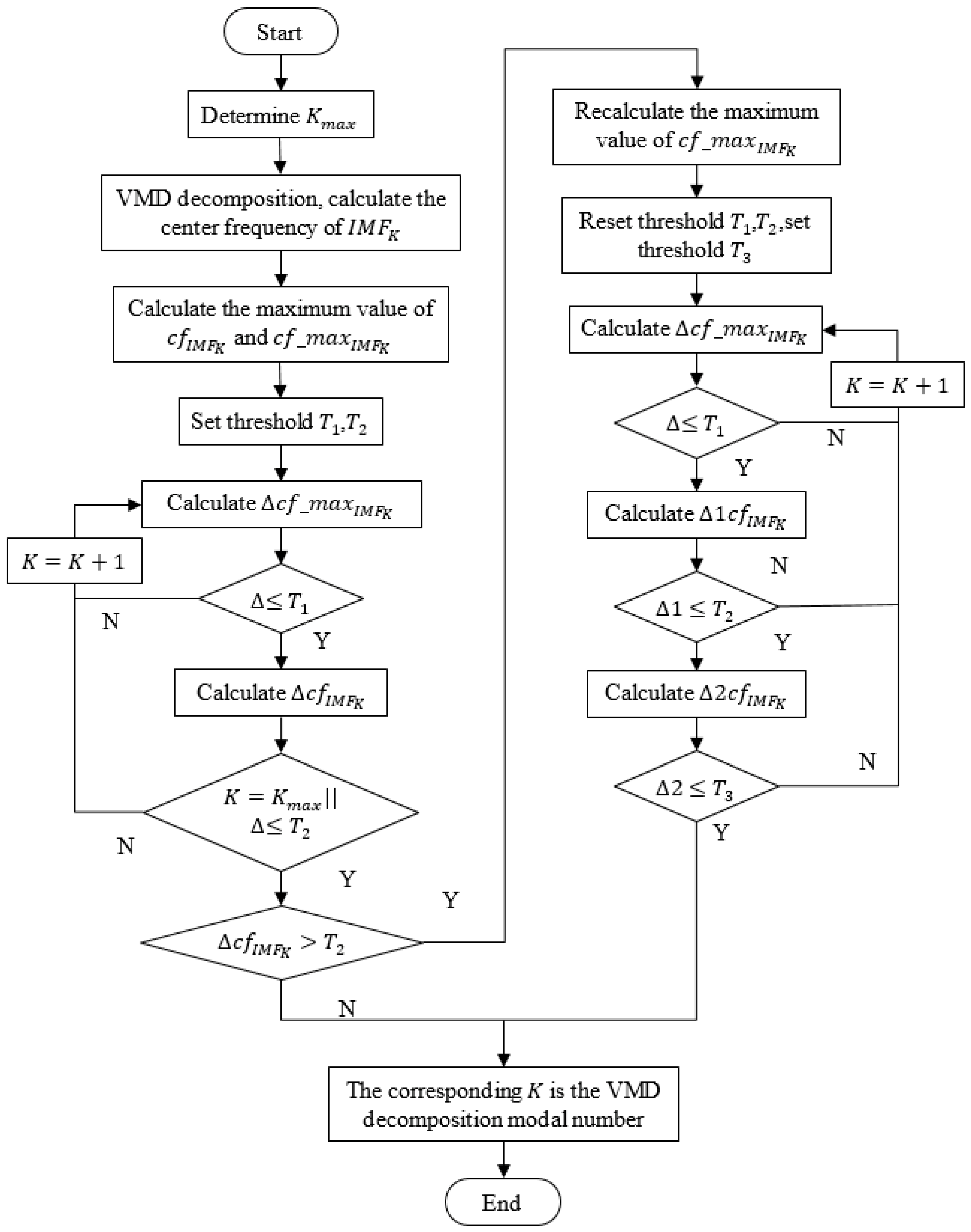
Each IMF component is obtained by using the VMD method, in which the decomposition corresponds to a central frequency, , and the centre frequency of the obtained IMF component under each scale is distributed from low frequency to high frequency. A center frequency method of the multi-threshold is proposed to determine the model number, K, of the VMD method (MTCFVMD). On the basis of the center frequency, the multi-threshold of , , and are set. The threshold, , is used to measure the difference between the maximum values of the central frequency under different scales and the maximum value of the center frequencies of all modes. For the central frequency method, it is known that the center frequency of the obtained IMF component under a certain scale is distributed from low frequency to high frequency. If the difference is greater than , it indicates that the maximum component of the central frequency in the original signal is not decomposed. The threshold, , is used to measure the difference between the value of the central frequency of the IMF component and the value of the central frequency of the IMF component under the same decomposition scale, K (). The VMD method can effectively decompose the two pure harmonic signals with a similar frequency, and the IMF components with a similar frequency are retained according to the threshold, . The threshold, , is used to measure the difference between the value of the central frequency of the IMF component and the value of the central frequency of the IMF component under the same decomposition scale, K (). The maximum value, , of the decomposition scale, K, is then set. The signal is decomposed under the decomposition scale, = 1, 2, …, , in order to obtain the value and the maximum value of the center frequency of the corresponding modes, and the maximum value of the center frequency of all modes under different scales. If the difference between the maximum value of the modal center frequency and the maximum value of all modal center frequencies is less than under a certain scale, K, the difference between the value of the center frequency of the IMF component and the value of the center frequency of the IMF component under the decomposition scale, K, is calculated (). If there is and the difference value is less than the threshold, , is judged. If not, the corresponding K is regarded as the optimal mode number of the VMD decomposition. If there is , the maximum value of all modal center frequencies is recalculated. If the difference between the maximum value of the modal center frequency and the maximum value of all modal center frequencies is less than under a certain scale, K, the difference between the value of the center frequency of the IMF component and the value of the center frequency of the IMF component under the decomposition scale, K, is calculated (). If the difference value is less than the threshold, , the difference between the value of the center frequency of the IMF component and the value of the center frequency of the IMF component under the decomposition scale, K, is calculated (). If the difference value is less than the threshold, , the value of K that meets the above conditions is regarded as the optimal mode number of the VMD decomposition method. The expressions of , , and are described as follows:
The flow of the improved VMD decomposition method based on the center frequency method of the multi-threshold is shown in Figure 1. The left half of the flow chart can determine the number of data modals of the inner and outer rings, and the right half can determine the number of data modals of the rolling element, indicating that the method has wide adaptability.
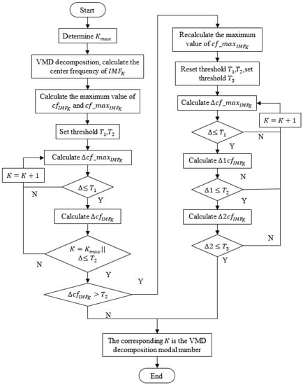
Figure 1.
The flow of the improved VMD (variational mode decomposition) decomposition component.
The implementation steps of the improved VMD method based on the center frequency method of the multi-threshold are described as follows:
- Step 1.
- Determine the maximum value, , of the decomposition scale.
- Step 2.
- The VMD method is used to decompose the original signal into a series of IMF components under different scales, . The center frequency value of each IMF component is calculated in order to obtain the set, .
- Step 3.
- Calculate the maximum value of the center frequency of the set, , under different scales, which is regarded as the .
- Step 4.
- Calculate the maximum value of the center frequency of the set, , which is regarded as the .
- Step 5.
- Set the threshold, (), ().
- Step 6.
- Calculate the difference between the maximum value of all modal center frequencies and the maximum value of the modal center frequency under the scale, K, which is regarded as . If there is , execute Step 7; if not, execute Step 6, .
- Step 7.
- Calculate the difference between the value of the center frequency of the IMF component and the value of the center frequency of the IMF component under the decomposition scale, K , which is regarded as . If there is , execute Step 8; if not, execute Step 6, ;
- Step 8.
- If there is , recalculate the maximum value of all modal center frequencies. Mark the value of the center frequency of the IMF component under the decomposition scale, K, as the maximum value of all modal center frequencies, , and execute Step 9. If not, the corresponding K is the optimal modal number of the VMD decomposition method .
- Step 9.
- Recalculate the thresholds, () and (), and set the threshold, ();
- Step 10.
- Calculate the difference between the maximum value of all modal center frequencies and the maximum value of the modal center frequency under the scale, K, which is regarded as . If , execute Step 11. If not, execute Step 10,
- Step 11.
- Calculate the difference between the value of the center frequency of the IMF component and the value of the center frequency of the IMF component under the decomposition scale, K , which is regarded as . If , execute Step 12. If not, execute Step 10, .
- Step 12.
- Calculate the difference between the value of the center frequency of the IMF component and the value of the center frequency of the IMF component under the decomposition scale, K, which is regarded as . If , the corresponding K is the optimal modal number of the VMD decomposition method. If not, execute Step 10, .
4. Fault Diagnosis Method of the Bearing Rolling Element
The improved VMD (MTCFVMD) algorithm and Hilbert transformation are introduced into the vibration signal of the motor bearing rolling element in order to propose a fault diagnosis method. The flow of the fault diagnosis method is shown in Figure 2.
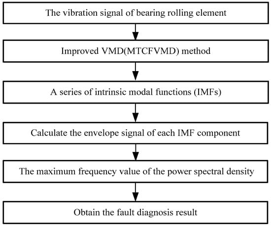
Figure 2.
The flow of the fault diagnosis method.
5. Analysis of Vibration Signals of the Motor Bearing Rolling Element
5.1. Effectiveness Analysis of the Center Frequency Method of the Multi-Threshold
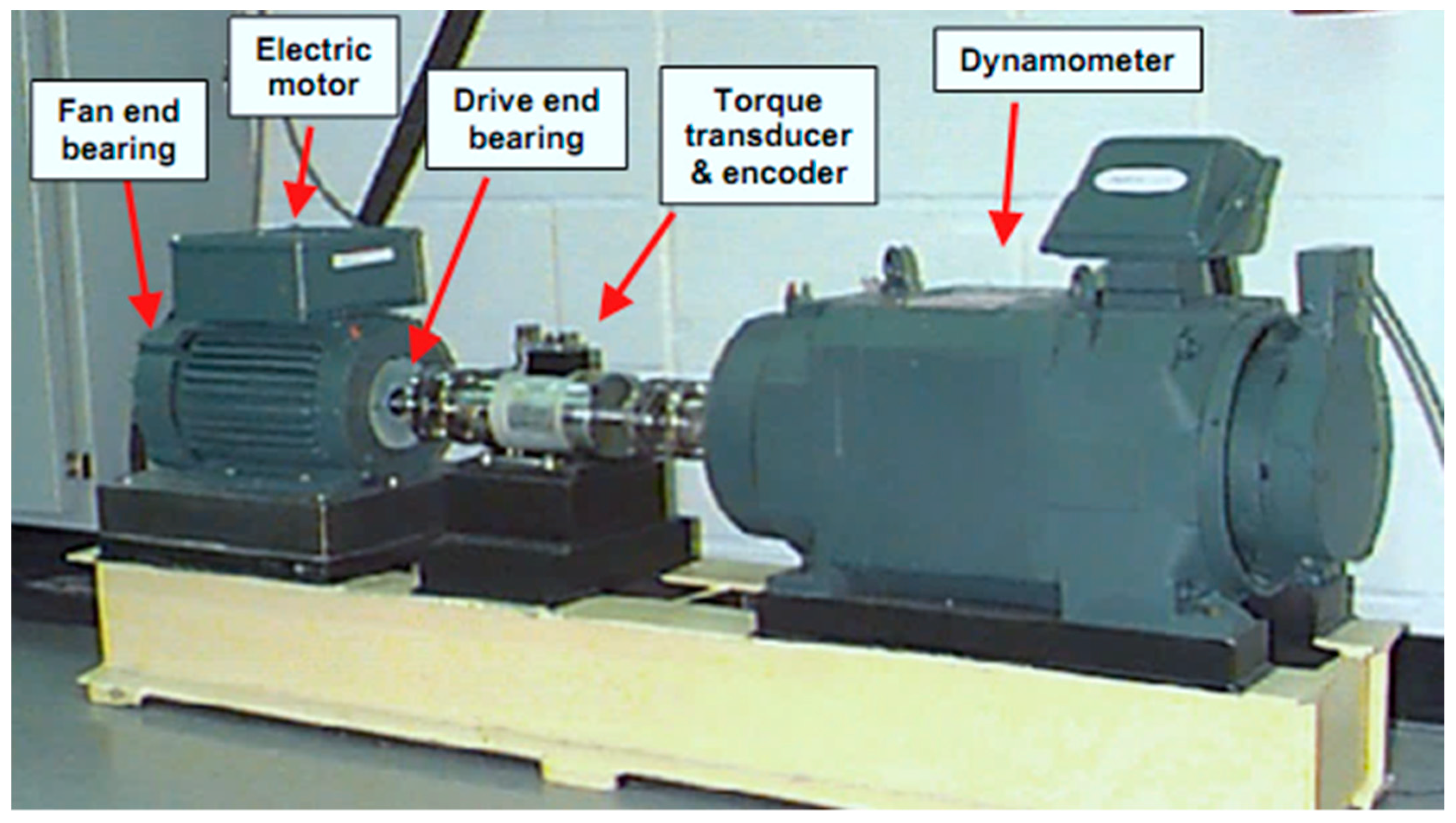
The motor bearing data came from the electrical engineering laboratory of Case Western Reserve University [82]. The deep groove ball bearing of 6205-2RS 6 JEM SKF[M1] (SKF company, Goteborg, Sweden) was used in this experiment. The experiment platform is shown in Figure 3. It used electro-discharge technology to machine a single point of damage on the bearing. The fault diameter was 0.1778 mm, the rotating speed was 1797 r/min, the sampling frequency was 12 kHz, and the signal length was 2048 points. The bearing information of the 6205-2RS JEM SKF deep groove ball bearing is described in Table 1.
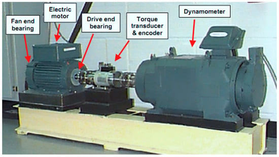
Figure 3.
The experiment platform [79].

Table 1.
The bearing information of the 6205-2RS JEM SKF deep groove ball bearing.
The fault characteristic frequency of the outer ring, , inner ring, , and the rolling element, , can been calculated by the theoretical formula as follows:
where is the axis revolution frequency (Hz), is the number of rolling elements, is the diameter of the rolling elements, is the pitch diameter of the rolling elements, and is the pressure angle of the rolling elements.
The theoretical calculation values of the fault characteristic frequency were calculated and are shown in Table 2.

Table 2.
Fault characteristic frequencies.
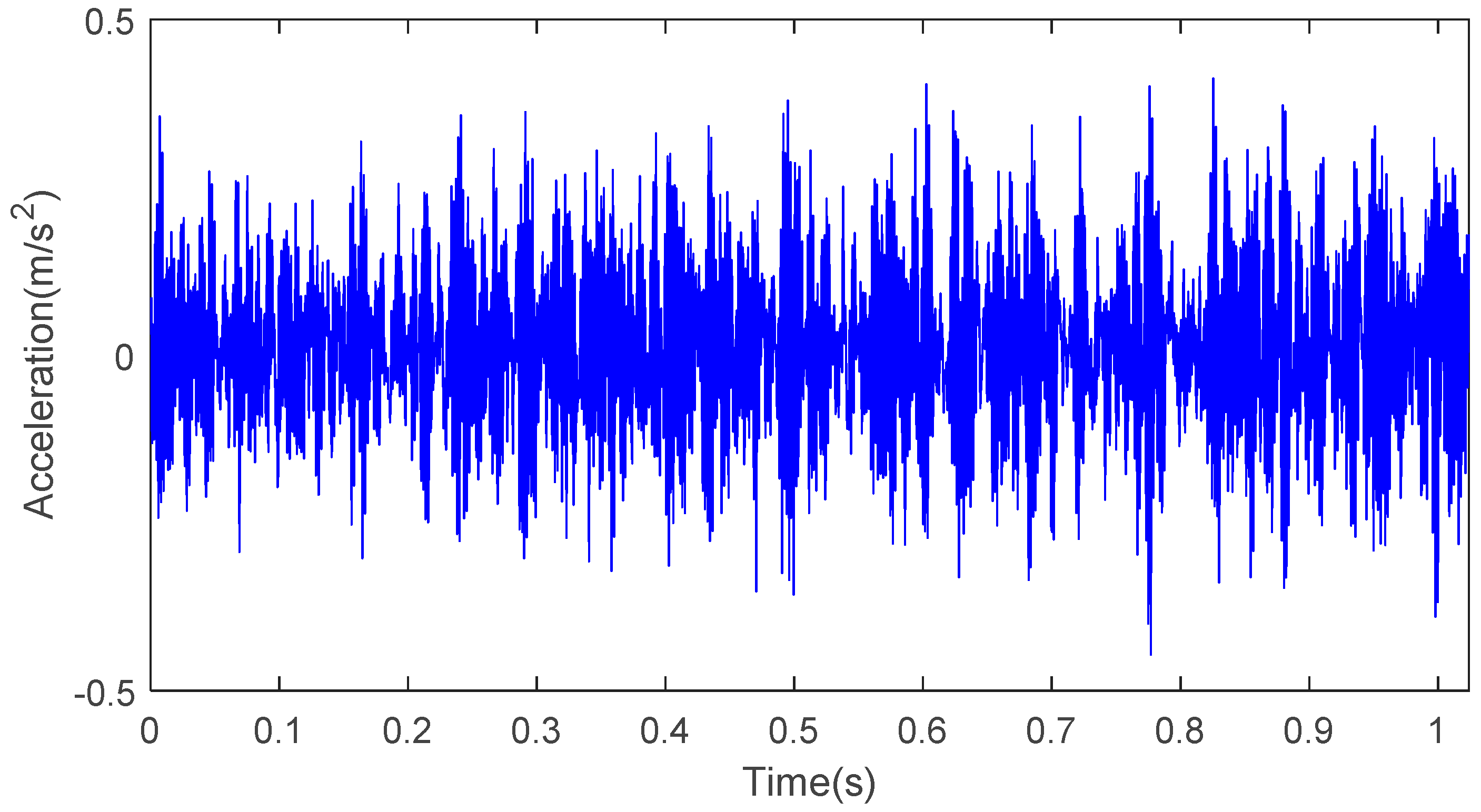
The time domain waveform and frequency domain waveform of the motor bearing rolling element fault signal under no-load are shown in Figure 4 and Figure 5.

Figure 4.
Time domain waveform.
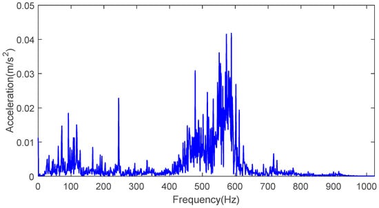
Figure 5.
Frequency domain waveform.
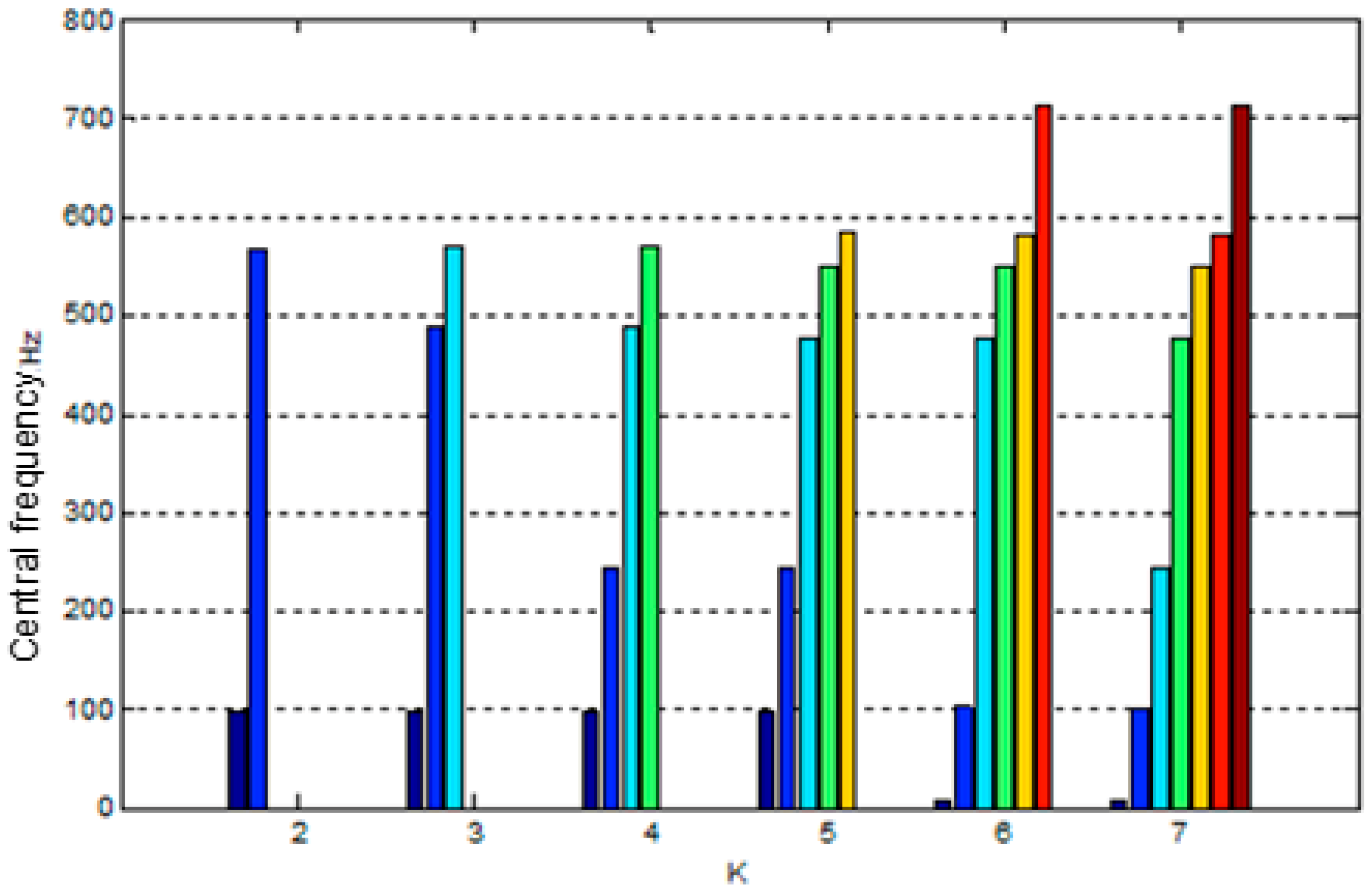
The improved VMD decomposition method was used to decompose the fault signal of a motor bearing rolling element under no-load, and the center frequency of each IMF component under different scales is shown in Figure 6.
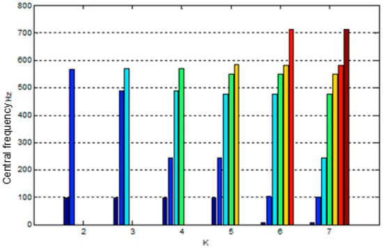
Figure 6.
Center frequency of each IMF (intrinsic modal functions) component under different scales.
The center frequency method of the multi-threshold was used to decompose the rolling element data in order to determine the modal number of the VMD decomposition. When K = 2, 3, 4, 5, the difference between the maximum value of the center frequency value of the corresponding mode under different scales and the maximum value of the center frequency of all modes is less than (), which is not met. When there is , the difference between the value of the center frequency of the IMF component and the value of the center frequency of the IMF component under the decomposition scale, K (), is less than or equal to (), which is not met, so the maximum value of all modal center frequencies was recalculated. It can be seen from Figure 3 that when K = 7, the center frequency of the seventh IMF component obtains the maximum value of all modal center frequencies, so the center frequency of the sixth IMF component is determined as the maximum value of all modal center frequencies, and the threshold was recalculated (), (), and the threshold set to . When K = 2, the difference between the maximum value of the center frequency value of the corresponding modes under different scales and the maximum value of the center frequency of all modes is less than or equal to (), which is not met. When K = 3, the difference between the center frequency of the IMF component and the IMF component (K = L) under the scale is less than or equal to ), which is not met. When K = 4, the condition of judgment is met at the same time, so K = 4 is the optimal modal number of VMD decomposition. Compared with the central frequency method, it can be seen that in the modals determined by the two methods, the number of decomposition modes is too large when K = 6, which results in false components and interference judgment, so K = 4 is better than K = 6.
5.2. Feature Extraction Based on the Hilbert Transform
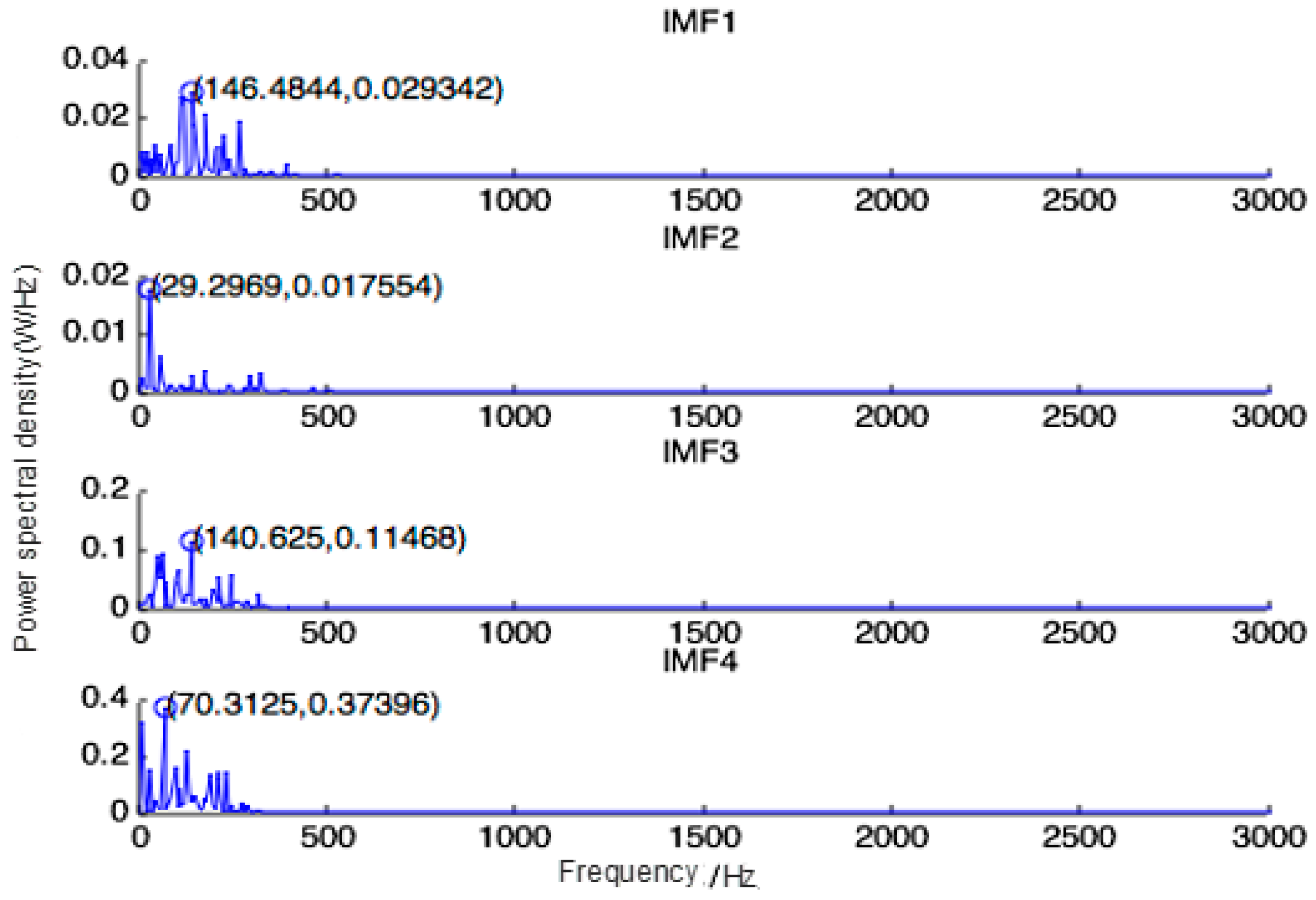
The power spectrum represents the relationship between signal power and frequency, that is, the distribution of signal power in the frequency domain. In this paper, the Hilbert transform was used to solve the envelope signal of each IMF component, then the power spectrum of the envelope signal was solved, and the frequency value with the largest power spectral density is marked in the figure, which was used to represent the fault characteristic frequency, rotating frequency, and frequency multiplication of the signal extracted by power spectrum analysis. The fault characteristic frequency of the motor bearing rolling element was 141.0751 Hz. The optimal modal number, K = 4, was determined according to the center frequency method of the multi-threshold. In order to verify the validity of the optimal modal number, for the motor bearing rolling element data, the power spectrum frequency values of each IMF component under K = 3, 4, and 5 are shown in Table 3.

Table 3.
The frequency values of the power spectrum of each IMF component.
As can be seen from Table 3, 29.2969 Hz represents the rotating frequency, 146.4844 Hz represents the rotating frequency of five times, 140.625 Hz represents the rolling element fault characteristic frequency, 70.3125 Hz represents the rolling element fault characteristic frequency of 1/2, and 11.7188 Hz represents the rolling element fault characteristic frequency of 1/12. The value of 52.7344 Hz represents the difference between the rolling element fault characteristic frequency and the frequency tripling of the rotating frequency. When k = 4, the four IMF components can obtain the rotating frequency, the rotating frequency of five times, the rolling element fault characteristic frequency, and the rolling element fault characteristic frequency of 1/2. When k = 3, the rotating frequency cannot be extracted. When k = 5, the rolling element fault characteristic frequency cannot be extracted. Therefore, k = 4 was determined as the optimal modal number of the VMD method for the rolling element data, and the power spectrum of the corresponding IMF component is shown in Figure 7.
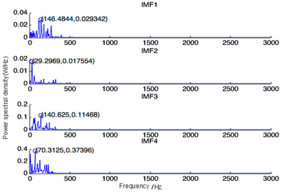
Figure 7.
Power spectrum of each IMF component under .
From the experimental results, it is proven that the validity of K is the optimal modal number of the VMD decomposition determined by the center frequency the of multi-threshold by solving the power spectrum in this paper.
5.3. Comparative Analysis of Different Methods
In order to verify the effectiveness of the improved VMD algorithm, the improved VMD algorithm was compared with the EMD and EEMD methods. The vibration signals of the motor bearing rolling element were decomposed by the improved VMD method, EMD method, and EEMD method, respectively, and the power spectrum of the IMF component was obtained. The effectiveness of the improved VMD method was proven by analyzing the effective frequency components of the power spectrum. The EMD method and the EEMD method were used, and when k = 4, the IMF components by the MTCFVMD method for the motor bearing rolling element fault data were obtained and the envelope signal of each IMF component was obtained by the Hilbert transform. The frequency value of the power spectrum of the envelope signal is shown in Table 4.

Table 4.
Comparative result of different methods for the rolling element fault (Hz).
As can be seen from Table 4, 29.2969 Hz represents the rotating frequency, 58.5938 Hz represents the frequency multiplication, 117.2 Hz represents the four times rotating frequency, 146.4844 Hz represents the rotating frequency of five times, 140.625 Hz represents the rolling element fault characteristic frequency, 70.3125 Hz represents the rolling element fault characteristic frequency of 1/2, 41.0156 Hz represents the difference between the rolling element fault characteristic frequency of 1/2 and the rotating frequency, and 234.375 Hz represents the difference between the rolling element fault characteristic frequency of 5/4 and the frequency multiplication. It can be seen from Table 4 that the number of effective frequencies obtained by solving the power spectrum of the IMF component decomposed by the EEMD method is more than that of the EMD method. Therefore, the decomposition effect of the EEMD method is better than the EMD method. Compared with the MTCFVMD method, the number of IMF components obtained by the MTCFVMD method is less than the EMD method and the EEMD method, and each modal can extract the effective frequency value. There were some invalid frequency values in the modes of the EMD method and the EEMD decomposition, so the decomposition effect of the MTCFVMD method is better than the EMD method and the EEMD method.
By comparing and analyzing the improved VMD method, it can be seen that the number of decomposition modals of the MTCFVMD method is less than that of the EMD and EEMD methods, which greatly reduces the running time. According to the power spectrum analysis, each IMF component obtained by the MTCFVMD method can extract effective frequency values, and some IMF components obtained by the EMD method and EEMD method cannot extract effective frequency values. It shows that the MTCFVMD method can effectively decompose the original signal, which proves the effectiveness and superiority of the MTCFVMD method.
6. Conclusions
The fault diagnosis method based on the VMD method with the center frequency method of the double threshold is used for the bearing inner and outer rings of a motor, however, this method contains difficulties when applying it to the rolling element of motor bearings. In this paper, a center frequency method of the multi-threshold was proposed to realize the adaptive determination of the modal decomposition number of the VMD method. Then, the envelope signal of each IMF component was obtained by the Hilbert transform, and the maximum frequency value of the power spectral density was obtained, which was used to obtain the fault characteristic frequency of the rolling element of the motor bearing. The rolling element vibration data of the rolling bearing of the motor was used to test the effectiveness of the proposed method. The experiment results showed that the center frequency method of the multi-threshold can effectively determine the number of decomposition components for the VMD method. Furthermore, it showed a higher decomposition accuracy and efficiency. At the same time, the fault diagnosis method based on the MTCFVMD method and Hilbert transformation can effectively and accurately extract the fault characteristics of the rolling element of a rolling bearing. Additionally, the extraction effect of the MTCFVMD method was better than those of the EMD method and the EEMD method.
Author Contributions
The methodology, H.L. and H.Z.; validation, H.Z. and W.D.; data curation, D.L.; writing—original draft preparation, S.Z.; writing—review and editing, H.L., Y.Y., H.Z., and W.D.; funding acquisition, H.Z., and W.D.
Funding
This work was supported by the National Natural Science Foundation of China (51605068, 61771087, 51879027, 51579024), the Innovative Talents Promotion Plan of Liaoning colleges and Universities (LR2017058) and Liaoning BaiQianWan Talents Program.
Acknowledgments
The authors would like to thank all the reviewers for their constructive comments. The program for the initialization, study, training, and simulation of the proposed algorithm in this article was written with the tool-box of MATLAB 2014b produced by the Math-Works, Inc.
Conflicts of Interest
The authors declare no conflict of interest.
References
- Qian, L.; Kang, M.; Fu, X.Q.; Wang, X.S.; Fei, X.G. Application of adaptive morphology in bearing fault diagnosis based on VMD. J. Vib. Shock 2017, 36, 227–233. [Google Scholar]
- Vafaei, S.; Rahnejat, H.; Aini, R. Vibration monitoring of high speed spindles using spectral analysis techniques. Int. J. Mach. Tools Manuf. 2002, 42, 1223–1234. [Google Scholar] [CrossRef]
- Deering, R.; Kaiser, J.F. The use of a masking signal to improve empirical mode decomposition. In Proceedings of the IEEE International Conference on Acoustics, Speech, and Signal Processing, Philadelphia, PA, USA, 23 March 2005; pp. 485–488. [Google Scholar]
- Liu, G.; Chen, B.; Gao, Z.; Fu, H.; Jiang, S.; Wang, L.; Yi, K. Calculation of joint return period for connected edge data. Water 2019, 11, 300. [Google Scholar] [CrossRef]
- Chen, H.L.; Xu, Y.T.; Wang, M.J.; Zhao, X.H. A balanced whale optimization algorithm for constrained engineering design problems. Appl. Math. Model. 2019, 71, 45–59. [Google Scholar] [CrossRef]
- Wardle, F.P. Vibration forces produced by waviness of the rolling surfaces of thrust loaded ball bearings Part 1: Theory. Proc. Inst. Mech. Eng. Part C J. Mech. Eng. Sci. 1988, 202, 305–312. [Google Scholar] [CrossRef]
- Ren, Z.R.; Skjetne, R.; Jiang, Z.Y.; Gao, Z.; Verma, A.S. Integrated GNSS/IMU hub motion estimator for offshore wind turbine blade installation. Mech. Syst. Signal Process. 2019, 123, 222–243. [Google Scholar] [CrossRef]
- Lu, S.L.; He, Q.B.; Zhao, J.W. Bearing fault diagnosis of a permanent magnet synchronous motor via a fast and online order analysis method in an embedded system. Mech. Syst. Signal Process. 2018, 113, 36–49. [Google Scholar] [CrossRef]
- Yu, J.; He, Y.J. Planetary gearbox fault diagnosis based on data-driven valued characteristic multigranulation model with incomplete diagnostic information. J. Sound Vib. 2018, 429, 63–77. [Google Scholar] [CrossRef]
- Yeh, C.H.; Shi, W.B. Identifying phase-amplitude coupling in cyclic alternating pattern using masking signals. Sci. Rep. 2018, 8, 2649. [Google Scholar] [CrossRef]
- Vafaei, S.; Rahnejat, H. Indicated repeatable runout with wavelet decomposition (IRR-WD) for effective determination of bearing-induced vibration. J. Sound Vib. 2003, 260, 67–82. [Google Scholar] [CrossRef]
- Liu, Y.Q.; Yi, X.K.; Chen, R.; Zhai, Z.G.; Gu, J.X. Feature extraction based on information gain and sequential pattern for English question classification. IET Softw. 2018, 12, 520–526. [Google Scholar] [CrossRef]
- Song, J.; Feng, Q.; Wang, X.; Fu, H.; Jiang, W.; Chen, B. Spatial association and effect evaluation of CO2 emission in the Chengdu-Chongqing urban agglomeration: Quantitative evidence from social network analysis. Sustainability 2019, 11, 1. [Google Scholar] [CrossRef]
- Lu, S.L.; Zhou, P.; Wang, X.X.; Liu, Y.B.; Liu, F. Condition monitoring and fault diagnosis of motor bearings using undersampled vibration signals from a wireless sensor network. J. Sound Vib. 2018, 414, 81–96. [Google Scholar] [CrossRef]
- Avargel, Y.; Cohen, I. Modeling and identification of nonlinear systems in the short-time Fourier transform domain. IEEE Trans. Signal Process. 2010, 58, 291–304. [Google Scholar] [CrossRef]
- Deng, W.; Yao, R.; Zhao, H.M.; Yang, X.H.; Li, G.Y. A novel intelligent diagnosis method using optimal LS-SVM with improved PSO algorithm. Soft Comput. 2019, 23, 2445–2462. [Google Scholar] [CrossRef]
- Yang, A.; Li, S.; Lin, H.; Jin, D. Edge extraction of mineralogical phase based on fractal theory. Chaos Solitions Fractals 2018, 117, 215–221. [Google Scholar]
- Luo, J.; Chen, H.L.; Zhang, Q.; Xu, Y.T.; Huang, H.; Zhao, X.H. An improved grasshopper optimization algorithm with application to financial stress prediction. Appl. Math. Model. 2018, 64, 654–668. [Google Scholar] [CrossRef]
- Ren, Z.; Skjetne, R.; Gao, Z. A crane overload protection controller for blade lifting operation based on model predictive control. Energies 2019, 12, 50. [Google Scholar] [CrossRef]
- Singh, J.; Darpe, A.K.; Singh, S.P. Rolling element bearing fault diagnosis based on over-complete rational dilation wavelet transform and auto-correlation of analytic energy operator. Mech. Syst. Signal Process. 2018, 100, 662–693. [Google Scholar] [CrossRef]
- Liu, G.; Chen, B.; Jiang, S.; Fu, H.; Wang, L.; Jiang, W. Double entropy joint distribution function and its application in calculation of design wave height. Entropy 2019, 21, 64. [Google Scholar] [CrossRef]
- Lynagh, N.; Rahnejat, H.; Ebrahimi, M.; Aini, R. Bearing induced vibration in precision high speed routing spindles. Int. J. Mach. Tools Manuf. 2000, 40, 561–577. [Google Scholar] [CrossRef]
- Zhou, Y.R.; Li, T.Y.; Shi, J.Y.; Qian, Z.J. A CEEMDAN and XGBOOST—Based approach to forecast crude oil prices. Complexity 2019, 2019, 4392785. [Google Scholar] [CrossRef]
- Gong, T.K.; Yuan, Y.B.; Yuan, X.H. Application of optimized multiscale mathematical morphology for bearing fault diagnosis. Meas. Sci. Technol. 2017, 28, 045401. [Google Scholar] [CrossRef]
- Su, J.; Sheng, Z.G.; Xie, L.B.; Li, G.; Liu, A.X. Fast splitting based tag identification algorithm for anti-collision in UHF RFID system. IEEE Trans. Commun. 2018, 67, 2527–2538. [Google Scholar] [CrossRef]
- Xie, H.M.; Zhang, L.B.; Li, H.Y.; Koppala, S.; Yin, S.; Li, S.; Yang, K.; Zhu, F. Efficient recycling of Pb from zinc leaching residues by using the hydrometallurgical method. Mater. Res. Express 2019. [Google Scholar] [CrossRef]
- Li, T.; Shi, J.; Li, X.; Wu, J.; Pan, F. Image encryption based on pixel-level diffusion with dynamic filtering and DNA-level permutation with 3D Latin cubes. Entropy 2019, 21, 319. [Google Scholar] [CrossRef]
- Yan, J.H.; Lu, L. Improved Hilbert-Huang transform based weak signal detection methodology and its application on incipient fault diagnosis and ECG signal analysis. Signal Process. 2014, 98, 74–87. [Google Scholar] [CrossRef]
- Borghesani, P.; Pennacchi, P.; Randall, R.B.; Sawalhi, N.; Ricci, R. Application of cepstrum pre-whitening for the diagnosis of bearing faults under variable speed conditions. Mech. Syst. Signal Process. 2013, 36, 370–384. [Google Scholar] [CrossRef]
- Hwang, Y.R.; Jen, K.K.; Shen, Y.T. Application of cepstrum and neural network to bearing fault detection. J. Mech. Sci. Technol. 2009, 23, 2730. [Google Scholar] [CrossRef]
- Kang, L.; Du, H.L.; Du, X.; Wang, H.T.; Ma, W.L.; Wang, M.L.; Zhang, F.B. Study on dye wastewater treatment of tunable conductivity solid-waste-based composite cementitious material catalyst. Desalin. Water Treat. 2018, 125, 296–301. [Google Scholar] [CrossRef]
- Deng, W.; Zhao, H.M.; Yang, X.H.; Xiong, J.X.; Sun, M.; Li, B. Study on an improved adaptive PSO algorithm for solving multi-objective gate assignment. Appl. Soft Comput. 2017, 59, 288–302. [Google Scholar] [CrossRef]
- Shen, L.; Chen, H.; Yu, Z.; Kang, W.; Zhang, B.; Li, H.; Yang, B.; Liu, D. Evolving support vector machines using fruit fly optimization for medical data classification. Knowl.-Based Syst. 2016, 96, 61–75. [Google Scholar]
- Park, S.; Kim, S.; Choi, J.H. Gear fault diagnosis using transmission error and ensemble empirical mode decomposition. Mech. Syst. Signal Process. 2018, 108, 262–275. [Google Scholar] [CrossRef]
- Zhao, H.M.; Yao, R.; Xu, L.; Yuan, Y.; Li, G.Y.; Deng, W. Study on a novel fault damage degree identification method using high-order differential mathematical morphology gradient spectrum entropy. Entropy 2018, 20, 682. [Google Scholar] [CrossRef]
- Zhu, Z.Y.; Peng, G.L.; Chen, Y.H.; Gao, H.J. A convolutional neural network based on a capsule network with strong generalization for bearing fault diagnosis. Neurocomputing 2019, 323, 62–75. [Google Scholar] [CrossRef]
- Yang, A.M.; Yang, X.L.; Chang, J.C.; Bai, B.; Kong, F.B.; Ran, Q.B. Research on a fusion scheme of cellular network and wireless sensor networks for cyber physical social systems. IEEE Access 2018, 6, 18786–18794. [Google Scholar]
- Guo, S.K.; Liu, Y.Q.; Chen, R.; Sun, X.; Wang, X.X. Improved SMOTE algorithm to deal with imbalanced activity classes in smart homes. Neural Process. Lett. 2018. [Google Scholar] [CrossRef]
- Chen, R.; Guo, S.K.; Wang, X.Z.; Zhang, T.L. Fusion of multi-RSMOTE with fuzzy integral to classify bug reports with an imbalanced distribution. IEEE Trans. Fuzzy Syst. 2019. [Google Scholar] [CrossRef]
- Wen, J.; Xu, Y.; Li, Z.; Ma, Z.; Xu, Y. Inter-class sparsity based discriminative least square regression. Neural Netw. 2018, 102, 36–47. [Google Scholar] [CrossRef]
- Fu, H.; Li, Z.; Liu, Z.; Wang, Z. Research on big data digging of hot topics about recycled water use on micro-blog based on particle swarm optimization. Sustainability 2018, 10, 2488. [Google Scholar] [CrossRef]
- Yu, W.; Zeng, Z.; Peng, B.; Yan, S.; Huang, Y.; Jiang, H.; Li, X.; Fan, T. Multi-objective optimum design of high-speed backplane connector using particle swarm optimization. IEEE Access 2018, 6, 35182–35193. [Google Scholar] [CrossRef]
- Yu, W.; Zeng, Z.; Peng, B.; Yan, S.; Huang, Y.; Jiang, H.; Li, X.; Fan, T. Robust sparse linear discriminant analysis. IEEE Trans. Circuits Syst. Video Technol. 2018, 29, 390–403. [Google Scholar] [CrossRef]
- Guo, S.K.; Chen, R.; Wei, M.M.; Li, H.; Liu, Y.Q. Ensemble data reduction techniques and multi-RSMOTE via fuzzy integral for bug report classification. IEEE Access 2018, 6, 5934–45950. [Google Scholar] [CrossRef]
- Zhao, H.M.; Sun, M.; Deng, W.; Yang, X.H. A new feature extraction method based on EEMD and multi-scale fuzzy entropy for motor bearing. Entropy 2017, 19, 14. [Google Scholar] [CrossRef]
- Zhang, Q.; Chen, H.; Heidari, A.A.; Zhao, X.; Xu, Y.; Wang, P.; Li, Y.; Li, C. Chaos-induced and Mutation-driven Schemes Boosting Salp Chains-inspired Optimizers. IEEE Access 2019, 7, 31243–31261. [Google Scholar] [CrossRef]
- Guo, S.K.; Chen, R.; Li, H.; Gao, J.; Liu, Y.Q. Crowdsourced Web application testing under real-time constraints. Int. J. Softw. Eng. Knowl. Eng. 2018, 28, 751–779. [Google Scholar] [CrossRef]
- Deng, W.; Xu, J.J.; Zhao, H.M. An improved ant colony optimization algorithm based on hybrid strategies for scheduling problem. IEEE Access 2019, 7, 20281–20292. [Google Scholar] [CrossRef]
- Deng, W.; Zhao, H.M.; Zou, L.; Li, G.Y.; Yang, X.H.; Wu, D.Q. A novel collaborative optimization algorithm in solving complex optimization problems. Soft Comput. 2017, 21, 4387–4398. [Google Scholar] [CrossRef]
- Zhou, J.C.; Du, Z.X.; Liao, Y.H.; Tang, A.H. An optimization design of vehicle axle system based on multi-objective cooperative optimization algorithm. J. Chin. Inst. Eng. 2018, 41, 635–642. [Google Scholar] [CrossRef]
- Smith, J.S. The local mean decomposition and its application to EEG perception data. J. R. Soc. Interface 2005, 2, 443–454. [Google Scholar] [CrossRef]
- Cheng, G.; Chen, X.H.; Li, H.Y. Study on planetary gear fault diagnosis based on entropy feature fusion of ensemble empirical mode decomposition. Measurement 2016, 91, 140–154. [Google Scholar] [CrossRef]
- Zhang, C.; Peng, Z.X.; Chen, S. A gearbox fault diagnosis method based on frequency-modulated empirical mode decomposition and support vector machine. Proc. Inst. Mech. Eng. Part C J. Mech. Eng. Sci. 2018, 232, 369–380. [Google Scholar] [CrossRef]
- Song, Y.H.; Zeng, S.K.; Ma, J.M. A fault diagnosis method for roller bearing based on empirical wavelet transform decomposition with adaptive empirical mode segmentation. Measurement 2018, 117, 266–276. [Google Scholar] [CrossRef]
- Zhou, Z.; Zhu, Y.S.; Zhang, Y.Y.; Zhu, C.F.; Wang, P. Adaptive fault diagnosis of rolling bearings based on EEMD and demodulated resonance. J. Vib. Shock 2013, 32, 76–80. [Google Scholar]
- Ding, J.M.; Zhao, W.T.; Miao, B.R.; Lin, J.H. Adaptive sparse representation based on circular-structure dictionary learning and its application in wheelset-bearing fault detection. Mech. Syst. Signal Process. 2018, 111, 399–422. [Google Scholar]
- Li, Z.P.; Chen, J.L.; Zi, Y.Y. Independence-oriented VMD to identify fault feature for wheel set bearing fault diagnosis of high speed locomotive. Mech. Syst. Signal Process. 2017, 85, 512–529. [Google Scholar] [CrossRef]
- Wang, Z.P.; Jia, L.M.; Qin, Y. Adaptive diagnosis for rotating machineries using information geometrical kernel-ELM based on VMD-SVD. Entropy 2018, 20, 73. [Google Scholar] [CrossRef]
- Lian, J.J.; Liu, Z.; Wang, H.J. Adaptive variational mode decomposition method for signal processing based on mode characteristic. Mech. Syst. Signal Process. 2018, 107, 53–77. [Google Scholar] [CrossRef]
- Zhang, X.; Miao, Q.; Zhang, H. A parameter-adaptive VMD method based on grasshopper optimization algorithm to analyze vibration signals from rotating machinery. Mech. Syst. Signal Process. 2018, 108, 58–72. [Google Scholar]
- Jiang, S.; Lian, M.; Lu, C.; Gu, Q.; Ruan, S.; Xie, X. Ensemble prediction algorithm of anomaly monitoring based on big data analysis platform of open-pit mine slope. Complexity 2018, 2018, 1048756. [Google Scholar] [CrossRef]
- Xu, J.F.; Ren, Z.R.; Li, Y.; Skjetne, R.; Halse, K.H. Dynamic simulation and control of anactive roll reduction system using free flooding tanks with vacuum pumps. J. Offshore Mech. Arct. Eng. 2018, 140, 061302. [Google Scholar]
- Xie, H.; Yang, K.; Li, S.; Yin, S.; Peng, J.; Zhu, F.; Li, H.; Zhang, L. Microwave heating-assisted pyrolysis of mercury from sludge. Mater. Res. Express 2019, 6, 015507. [Google Scholar] [CrossRef]
- Huang, F.; Yao, C.; Liu, W.; Li, Y.; Liu, X. Landslide susceptibility assessment in the nantian area of china: A comparison of frequency ratio model and support vector machine. Geomat. Nat. Hazards Risk 2018, 9, 919–938. [Google Scholar] [CrossRef]
- Sun, F.R.; Yao, Y.D.; Li, X.F. The heat and mass transfer characteristics of superheated steam coupled with non-condensing gases in horizontal wells with multi-point injection technique. Energy 2018, 143, 995–1005. [Google Scholar] [CrossRef]
- Sun, F.R.; Yao, Y.D.; Chen, M.Q.; Li, X.F.; Zhao, L.; Meng, Y.; Sun, Z.; Zhang, T.; Feng, D. Performance analysis of superheated steam injection for heavy oil recovery and modeling of wellbore heat efficiency. Energy 2017, 125, 795–804. [Google Scholar] [CrossRef]
- Xiao, L.; Zhang, X.H.; Lu, S.L.; Xia, T.B.; Xi, L.F. A novel weak-fault detection technique for rolling element bearing based on vibrational resonance. J. Sound Vib. 2019, 438, 490–505. [Google Scholar] [CrossRef]
- Cheng, C.; Qiao, X.Y.; Luo, H.; Teng, W.X.; Gao, M.L.; Zhang, B.C.; Yin, X.J. A semi-quantitative information based fault diagnosis method for the running gears system of high-speed trains. IEEE Access. 2019, 7, 38168–38178. [Google Scholar] [CrossRef]
- Yu, J.; Xu, Y.G.; Yu, G.B.; Liu, L.F. Fault severity identification of roller bearings using flow graph and non-naive Bayesian inference. Proc. Inst. Mech. Eng. Part C J. Mech. Eng. Sci. 2019. [Google Scholar] [CrossRef]
- Yu, J.; Ding, B.; He, Y.J. Rolling bearing fault diagnosis based on mean multigranulation decision-theoretic rough set and non-naive Bayesian classifier. J. Mech. Sci. Technol. 2018, 32, 5201–5211. [Google Scholar] [CrossRef]
- Wen, J.; Han, N.; Fang, X.; Fei, L.; Yan, K.; Zhan, S. Low-rank preserving projection via graph regularized reconstruction. IEEE Trans. Cybern. 2018, 49, 1279–1291. [Google Scholar] [CrossRef] [PubMed]
- Lei, Y.G.; Lin, J.; He, Z.J. A review on empirical mode decomposition in fault diagnosis of rotating machinery. Mech. Syst. Signal Process. 2013, 35, 108–126. [Google Scholar] [CrossRef]
- Guo, J.H.; Mu, Y.; Xiong, M.D.; Liu, Y.Q.; Gu, J.X. Activity feature solving based on TF-IDF for activity recognition in smart homes. Complexity 2019, 2019, 5245373. [Google Scholar] [CrossRef]
- Lu, S.L.; Qin, Y.; Hang, J.; Zhang, B.H.; Wang, Q.J. Adaptively estimating rotation speed from DC motor current ripple for order tracking and fault diagnosis. IEEE Trans. Instrum. Meas. 2019, 68, 741–753. [Google Scholar] [CrossRef]
- Zhao, H.T.; Mu, X.L.; Zheng, C.H.; Liu, S.J.; Zhu, Y.Q.; Gao, X.; Wu, T. Structural defects in 2D MoS2 nano-sheets and their roles in the adsorption of airborne elemental mercury. J. Hazard. Mater. 2019, 366, 240–249. [Google Scholar] [CrossRef] [PubMed]
- Deng, W.; Zhang, S.J.; Zhao, H.M.; Yang, X.H. A novel fault diagnosis method based on integrating empirical wavelet transform and fuzzy entropy for motor bearing. IEEE Access 2018, 6, 35042–35056. [Google Scholar] [CrossRef]
- Zhang, Q.; Chen, H.; Luo, J.; Xu, Y.; Wu, C.; Li, C. Chaos enhanced bacterial foraging optimization for global optimization. IEEE Access 2018, 6, 64905–64919. [Google Scholar] [CrossRef]
- Wu, D.Q.; Huo, J.Z.; Zhang, G.F.; Zhang, W.H. Minimization of logistics cost and carbon emissions based on quantum particle swarm optimization. Sustainability 2018, 10, 3791. [Google Scholar] [CrossRef]
- Zheng, J.; Pan, H.; Yang, S.; Cheng, J. Adaptive parameterless empirical wavelet transform based time-frequency analysis method and its application to rotor rubbing fault diagnosis. Signal Proces 2017, 130, 305–314. [Google Scholar] [CrossRef]
- Lu, S.L.; Yan, R.Q.; Liu, Y.B.; Wang, Q.J. Tacholess speed estimation in order tracking: A review with application to rotating machine fault diagnosis. IEEE Trans. Instrum. Meas. 2019. [Google Scholar] [CrossRef]
- Dragomiretskiy, K.; Zosso, D. Variational mode decomposition. IEEE Trans. Signal Process. 2014, 62, 531–544. [Google Scholar]
- Bearing Data Center. Available online: http://csegroups.case.edu/bearingdatacenter/home (accessed on 18 July 2018).
© 2019 by the authors. Licensee MDPI, Basel, Switzerland. This article is an open access article distributed under the terms and conditions of the Creative Commons Attribution (CC BY) license (http://creativecommons.org/licenses/by/4.0/).

