A Low-Cost Add-On Sensor and Algorithm to Help Small- and Medium-Sized Enterprises Monitor Machinery and Schedule Processes

Abstract

Since the concept of Industry 4.0 emerged, an increasing number of major manufacturers have incorporated relevant technologies to monitor machinery and schedule processes so as to increase yield and optimize production. However, most machinery monitoring technologies are far too expensive for small- and medium-sized enterprises. Furthermore, the production processes at small- and medium-sized enterprises are simpler and can thus be optimized without excessively complex scheduling systems. This study therefore proposed the use of cheaper add-on sensors for monitoring machinery and integrated them with an algorithm that can more swiftly produce results that meet multiple objectives. The proposed algorithm is meant to extend the capabilities of small- and medium-sized enterprises in monitoring machinery and scheduling processes, thereby enabling them to contend on an equal footing with larger competitors. Finally, we performed an experiment at an actual spring enterprise to demonstrate the validity of the proposed algorithm.

1. Introduction

Since the term Industry 4.0 was coined, an increasing number of major manufacturers have incorporated relevant technologies, such as using well-designed and embedded sensors to collect data from machinery or the test results of various products. Then, a server receives the signal from multiple sensors, and unifies the format of these signals, for monitoring, scheduling, and analysis [1,2]. This makes it possible for enterprises to monitor the operational status of machinery on an ongoing basis, and in so doing enhance production efficiency, reduce maintenance costs, and optimize quality. Industry 4.0 protocols can indeed help enterprises to improve performance and reduce costs; however, the capital outlay required for the adoption of these technologies (e.g., sensors, cloud computing, big data analysis) can be prohibitively high. Furthermore, the base infrastructure differs greatly from that of conventional enterprises, thereby necessitating considerable upgrades prior to implementation. Most large-scale enterprises are able to make these changes without difficulty; however, most small- and medium-sized enterprises (SMEs) are unable to absorb the costs.

Many researchers have sought to lower the adoption threshold for Industry 4.0. Dassisti et al. [3] introduced a core-meta model to help SMEs implement Industry 4.0 in their enterprises. Uriarte et al. [4] used the technique of mechanistic modeling to predict the micromilling cutting forces. Rivelo et al. [5] used the internal signals of machinery to do the tool wear detection. Plapper and Weck [6] proposed a new approach on using digital drive signals for monitoring the conditions of machine tool. Barrio et al. [7] discussed how to use the concept of Industry 4.0 to do modeling and process monitoring on machines. Finally, Birkel et al. [8] developed a risk framework for enterprises considering switching over to Industry 4.0.

It should be noted that most of the methods used to monitor machinery are impractical for SMEs, due to budgetary restrictions on the purchase of updated machinery equipped with the latest sensors. Moreover, it is doubtful that they will purchase large numbers of the same machines at the same time. To save money, the machines that they buy may even come from different manufacturers and countries. Consequently, these are reasons why mutual communication among machines is difficult for SMEs. Even if their machines had sensors that could send signals to the server, the formats of these signals vary and are almost impossible to analyze. In other words, it is extremely difficult for SMEs to introduce Industry 4.0 technologies [9,10]. Without these monitoring technologies, the gap between their yield and production costs and those of large manufacturers will gradually widen, and ultimately they will be unable to escape the fate of elimination. Some new methods are needed to address this issue. Such methods must be inexpensive so that they are affordable by SMEs with little capital.

Optimizing process schedules plays a significant role in Industry 4.0 technologies. For this reason, a number of researchers have proposed scheduling-related algorithms [11,12]. For instance, Kyparisis and Koulamas [12] proposed a multi-stage scheduling algorithm that can process multiple machineries running in parallel. Furthermore, they demonstrated that this problem is an NP-hard problem. Next, Tahar et al. [13] presented an algorithm that can schedule a set of independent jobs; the algorithm enables users to set the time, break up jobs, and complete them in the shortest time. In recent years, Ivanov et al. [11] developed a scheduling algorithm that can optimize job schedules and consider machinery statuses at the same time. Another feature of their algorithm is that it can assist enterprises in finding multi-objective results rather than the single-objective results in previous papers. As a result, their algorithm can provide enterprises with a variety of options and satisfy options under different conditions. Nevertheless, it is important to understand that although the method above solves the problem of scheduling optimization in Industry 4.0, it is too complex for SMEs. This is because most of these enterprises, which may produce products such as screws, springs, molds, or plastic injections, need only one step to complete the manufacturing of their products. A multi-stage algorithm would be too time-consuming, and these SMEs rarely have the budget to purchase relevant software and hardware to perform these calculations. Thus, some simple approaches are needed to solve this problem.

In response to these machinery monitoring and scheduling issues, this study proposed two solutions. First, in terms of monitoring, we present arduino-based add-on sensors to monitor machinery status. Then a feature extraction algorithm and a dimensionality reduction algorithm are utilized on these collected signals. Finally, a neural network is used to determine whether machinery statuses are normal. The advantage of this method is that the arduino-based add-on sensors are extremely inexpensive, so even if an enterprise requires a large quantity of these sensors, their cost will not be a great burden. Of course, the precision of the data collected by the arduino-based add-on sensors is not as high as that of data collected by expensive sensors. However, the products of SMEs, such as screws, springs, molds, or plastic products, do not require very high precision, so these add-on sensors are adequate for monitoring.

Second, in terms of scheduling, multi-objective scheduling is the current trend [11]. Therefore, we developed an algorithm for scheduling with multiple objectives. To achieve this goal, we incorporated the recently well-known skyline query [14,15,16], which can consider situations with different conditions and send back the optimal solutions for various combinations of conditions. With Table 1 and Figure 1 as an example, Table 1 presents the total work time and costs of different schedules. For instance, the total work time of Schedule 1 is 560 min, and its total cost is USD 2,500. Figure 1 displays the total work time and cost of each schedule in Table 1 using coordinates; each point represents a schedule. The points in the very lower left corner of Figure 1 (i.e., Schedules 1,3, and 4) are the skyline schedule results. Schedule 1 has the shortest total work time, Schedule 4 has the lowest total cost, and the total work time and cost of Schedule 3 falls between those of Schedules 1 and 4. Schedule 2 is not a skyline schedule result because its total work time and cost are both higher than those of Schedule 1. Enterprise workers will certainly choose Schedule 1 over Schedule 2. With the concept of skyline schedules, we can help enterprises identify schedules that are superior in all aspects. However, skyline queries are known for requiring longer computation time; to resolve this issue, we developed an innovative algorithm.

Table 1. The example of skyline schedules.

Schedule	Cost	Total Work Time
1	USD 2500	450 min
2	USD 3000	1400 min
3	USD 2000	670 min
4	USD 1000	800 min
5	USD 4500	500 min
6	USD 7300	650 min
7	USD 12,000	1400 min

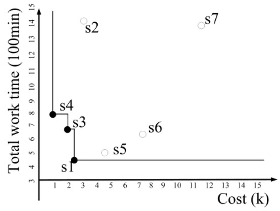
Figure 1. The example of skyline schedules.

This paper is arranged as follows. We first introduce some related work in Section 2. Section 3 explains the approaches for monitoring the machinery. Section 4 studies the methods for scheduling. Section 5 presents the experiment and discussion, and Section 6 contains the conclusion.

2. Related Works

2.1. Industry 4.0 in Small- and Medium-Sized Enterprises

Industry 4.0 initially enjoyed an enthusiastic response; however, many small- and medium-sized enterprises (SMEs) have been unable to participate in this movement due to prohibitively high adoption costs. This has led many researchers to look for ways to lower the entry threshold for SMEs. In the following, we examine a number of the aspects pertaining to the adoption of Industry 4.0 standards by SMEs.

One of the major issues is industrial performance objectives, which deal with flexibility, productivity, and delivery times [9]. Many enterprises seek to synchronize various flows through the supply chain; however, that requires considerable flexibility in responding to rapid market fluctuations. Peng et al. [17] proposed a real-time production flow scheme by which to modify production plans in accordance with changes in demand or disruptions in flow. Chalal et al. [18], introduced a model with one subsystem for modeling demand and another subsystem for modeling production, making it easier for firms to react to client demands.

Another major issue in the adoption of Industry 4.0 standards is productivity. Givehchi [19] sought to improve efficiency by sequencing machining tasks in a more efficient manner. Dombrowski and Ernst [20] simulated various growth scenarios at the enterprise-level with the aim of reconfiguring production lines to improve production flows. Other researchers focused on reducing delivery times by synchronizing production processes using cloud computing platforms. Denkena et al. [21] used the Internet of Things (IoT) to improve production flows by focusing on waiting times and bottlenecks as a guide for system reconfiguration.

A third major issue in the adoption of Industry 4.0 standards is industrial managerial capacity; that is, monitoring, control, and optimization. Monitoring system status is meant to facilitate proactive responses. For example, Denkena et al. [21] used the IoT to measure the real time flow of parts, whereas Velandia et al. [22] used Radio Frequency Identification (RFID) to record data throughout the entire production process. Control refers to the interaction between employees and the system using historical data and predetermined thresholds [9]. For example, MacKerron et al. [23] proposed an RFID-based system to monitor supply processes and automatically alert managers of impending inventory shortfalls. Optimization refers to efforts aimed at improving systems and processes. However, despite the numerous methods that could be employed to reach this goal, most previous work related to SMEs focused on simulating current industrial practices [18,24].

2.2. Feature Extraction and Dimensionality Reduction

Feature extraction and dimensionality reduction [25] are the preprocessing methods most commonly used in the analysis of signals such as those related to speech and activity recognition. Feature extraction refers to the identification of specific characteristics or patterns within a given signal. For example, the average value of a speech signal could be used to indicate the loudness of speech. The features used in the analysis of signals include mean values, correlations among axes, mean absolute deviation, root mean square, variance, standard deviation, signal magnitude area, and average energy. It should be noted however that the choice of feature set depends on the specifics of the case; that is, not all features are relevant, and irrelevant features can increase the execution time and/or undermine the precision of analysis [25]. Following feature extraction, a number of methods can be used to identify the features best suited to the analysis of a given case.

Dimensionality reduction is the method most commonly used in the selection of features suitable for the analysis of a particular signal. For example, dimensionality reduction can be used to sort through a large number of features identified in the signals collected by automated sensors, such as those found on various forms of machinery. This makes it possible to identify the features best able to verify that a machine is working smoothly or identify cases of imminent failure. Dimensionality reduction is commonly implemented using principal component analysis (PCA) [26] or linear discriminant analysis (LDA) [25]. PCA is an unsupervised method, whereas LDA is a supervised method. PCA is used to identify the projections best suited to “representing data”, whereas LDA is used for “discriminating among data” [27,28]. This makes LDA more suitable than PCA for the monitoring of machinery status.

2.3. Classifier for Recognizing the Status of Signal

Classifiers are among the most useful tools for the recognition of signal status. A classifier is first trained using well-defined features, the corresponding status of which is stipulated by experts. This makes it possible to use a trained classifier to determine the status of a signal based solely on its features. The most common classifiers include decision trees [29], K-nearest neighbors (KNN) [30], and neural networks [31]. Bao et al. [29] formulated the C4.5 decision tree to recognize 20 daily activities performed by humans. Karantonis et al. [32] developed an hierarchical binary classifier to enhance the precision of classification and recognition rates. Unfortunately, the computational and memory requirements of decision trees make them inapplicable in most real-world situations. Kose et al. [30] and Kaghyan and Sarukhanyan [33] achieved good results using KNN to deal with signals collected associated with human activities; however, the effectiveness of KNN can be compromised by a small training dataset and computational overhead limits its applicability.

Neural networks are currently the most popular method used in the recognition of signal status [34,35,36], due to their excellent learning capability in the discrimination of nonlinearly separable classes. Watanabe [36] used a feedforward neural network with triaxial accelerometer to recognize the movements of hemiplegic patients. Jatoba et al. [34] utilized an adaptive neuro-fuzzy inference system based on signals collected from a triaxial acceleration sensor. Yang et al. [25] recently merged a fuzzy system with a neural network to identify human activities based on signals collected using only one accelerometer. The results of these studies demonstrate the efficacy of using neural-network-based techniques for signal recognition.

2.4. Scheduling

Scheduling can be used in enterprises to optimize job flow by arranging tasks in a suitable order. Blazewicz et al. [37] and Lauff and Werner [38] discussed the problem of scheduling in multi-stage systems. Kyparisis and Koulamas [12] considered the same problem, while taking into account the effect of machinery processing speed on job flow. Tahar et al. [13] considered a scheduling problem in which jobs can be split up and assigned sequence-dependent setup times. These methods have proven effective in many situations; however, they are applicable only to single-objective scheduling problems. Ivanov et al. [11] proposed a multi-objective, multi-stage flexible scheduling problem using in each stage alternative machineries with different time-dependent processing speeds.

2.5. Skyline Query

Skyline query algorithms are quickly becoming the mainstay of decision support systems. They function as an alternative to top-k algorithms, which are unable to retain the characteristic features of the various dimensions. The skyline approach makes it possible to identify the best result for every dimension, and tailor the results according to criteria designated by the user. Consider a situation in which the user seeks accommodation close to a particular venue. As shown in Table 2, various forms of information pertaining to nearby hotels must be taken into account in the selection of accommodation. If cost and location were the only considerations, then the information could be arranged within a two-dimensional scatter diagram, as shown in Figure 2. The black line is the skyline; it indicates that the cost and distance of C are better than those of D. In other words, C dominates D on both criteria. Unfortunately, a skyline algorithm is unable to choose between A and C, due to the fact that C is closer to the desired venue but A has a lower price. In this situation, the skyline query would return both hotels, leaving the ultimate decision up to the user. This problem becomes increasingly complex when the number of criteria grows. For example, hotels A and C could all be considered skyline hotels, due to the fact that they are not dominated by other hotels.

Table 2. Information pertaining to hotels in the vicinity of the beach.

Hotel	Cost	Distance to the Beach	Internet Ratings
A	$100	5 km	3
B	$750	3.5 km	4
C	$230	1 km	3
D	$450	2 km	1
E	$320	8 km	3

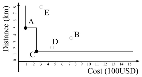
Figure 2. The example of skyline hotels.

Three skyline algorithms are particularly well known: block nested loops (BNL) [39], divide and conquer (DAC) [39], and sort limit skyline (SaLSa) [14]. The BNL algorithm compares a pair of data points and eliminates the point that is dominated. All of the remaining data points are then compared to one another iteratively in order to identify a single dominant candidate. This is the simplest and most intuitive skyline method; however, computational complexity grows exponentially with an increase in the quantity of data.

The DAC algorithm [39] breaks down data into groups, conducts a separate skyline query in each group, and then combines the group results into a final skyline query to produce a final decision. The elimination of many data points during the initial grouping process enhances the execution speed.

The SaLSa algorithm [14] uses summation values obtained from the raw data as threshold values to enable the filtering out of unnecessary data points. This algorithm arranges data sequentially according to the summation values and checks whether a given data point falls within the skyline threshold before testing for dominance; that is, only those below the threshold value are tested for dominance. The SaLSa algorithm has proven particularly effective in time and cost reduction.

3. Machinery Monitoring

In this chapter, we introduce a novel method for monitoring the status of machinery. The monitoring process involves the following steps: (1) collection of signals pertaining to machinery status using add-on sensors; (2) filtering and normalization of collected signals; (3) extraction of feature values and the export of each piece of data as a data point using windows with a designated range; (4) dimensionality reduction using LDA; and (5) input of results into neural network for training and generation of neural network parameters to enable the recognition of data pertaining to machinery status.

3.1. Add-On Sensors for the Collection of Data Related to Machinery Status

A number of researchers [40,41] have proposed the analysis of vibration data as a means by which to monitor the status of machines. In this study, we developed a monitoring system based on an inexpensive single chip controller, Arduino, in conjunction with triaxial accelerometers, infrared sensors, and temperature sensors. The proposed system is inexpensive and extensible, making it ideal for SMEs.

3.2. Filtering and Normalization of Collected Signals

The signals collected from accelerometers are filtered to remove noise prior to feature value calculation. To deal with the various forms of noise found in different machinery, we use the main frequency of the carrier signal for the selection of filter parameters. For example, if the frequency of the carrier were around 10 Hz, then a low-pass filter would be employed for the removal of noise.

3.3. Feature Extraction

The calculation of feature values is achieved using a window with data length determined by the user, such as an enterprise employee. Generally, the length should not exceed half the wavelength of the signal. In accordance with the recommendations in a previous study [25], 50% of each window is overlapped by the following window to enhance the precision of recognition. Figure 3 presents an example in which the signal was collected from a machine in a spring manufacturing facility. Based on a signal wavelength of approximately 200 Hz, the length of the window is set to 80 points with a 40-point overlap of the preceding and succeeding windows.

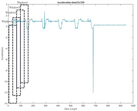
Figure 3. Example of feature extraction using windows.

Window values are represented as [X₁, X₂, …, X_|w|], where |W| refers to the length of a window, and extracted features are presented as follows:

• Mean: Mean value of signal data in each window
• Energy: Sum of squares of data in each window divided by the window length:

  $$\mathrm{Energy}=\frac{{\displaystyle {\sum }_{i=1}^{\left|W\right|}{\left|X_i\right|}^2}}{\left|W\right|},$$

  (1)
• Root mean square:

  $$\mathrm{RMS}=\sqrt{\frac{1}{\left|W\right|}{\displaystyle {\sum }_{i=1}^{\left|W\right|}{x}_i^2}}$$

  (2)
• Variance:

  $$\mathrm{variance}=\frac{1}{\left|W\right|-1}{\displaystyle {\sum }_{i=1}^{\left|W\right|}{(x_i-m)}^2},$$

  (3)

  where m is the mean value of Xi.
• Average absolute deviation:

  $$\mathrm{MAD}=\frac{1}{\left|W\right|}{\displaystyle {\sum }_{i=1}^{\left|W\right|}\left|x_i-m\right|}.$$

  (4)
• Standard deviation: Root mean square of variance
• Maximum value: Maximum value of each window.

3.4. Dimensionality Reduction Using LDA

In a system using triaxial accelerometers, infrared sensors, and temperature sensors, the following 5 signals would be received at one time: triaxial accelerometer (3 signals), infrared sensor (1 signal), and temperature sensor (1 signal). Extracting 7 features from each signal would result in a total of 35 features. However, this may also include irrelevant data, which could compromise recognition performance. Thus, we employ dimensionality reduction using LDA, which maps high-dimensional data onto a calculated vector, separates data into various categories, and tightens up data in each category. Dimensions with high feature value are then output as results. We adopted the two dispersion matrices outlined in [25], including covariance matrix S_B for between categories and covariance matrix S_W within categories. S_B is the predicted discrete vector values near the mixed averages, which is obtained as follows:

$$S_B={\displaystyle {\sum }_{\alpha =1}^N{n}_{\alpha }\left(m^{\alpha }-m\right){\left(m^{\alpha }-m\right)}^T}$$

(5)

and S_W is the predicted vector dispersion sample of each category, which is obtained as follows:

$$S_W={\displaystyle {\sum }_{\alpha =1}^N{n}_{\alpha }{\displaystyle {\sum }_{i=1}^{n_{\alpha }}\left(x_i{}^{\alpha }-m^{\alpha }\right){\left(x_i{}^{\alpha }-m^{\alpha }\right)}^T}}$$

(6)

where N denotes the number of categories; n_α is the number of samples in category α; x_i^α represents sample i of category α; m^α is the sample mean vector of category α, and m is the mean vector of all data. LDA produces mapping vector w to store the category integrity under low dimensionality, and w is used to maximize the formula below; that is, it maximizes the covariance between different categories and minimizes the covariance within a single category. In other words, the objective is to maximize J(w) in Equation (7). Once w has been calculated, the data can be mapped onto coordinate systems and new coordinates can be identified to reduce dimensionality

$$J\left(w\right)=\frac{w^T{s}_{B}w}{w^T{s}_{w}w}$$

(7)

Using Figure 3 as an example of dimensionality reduction, we can obtain the results in Figure 4, in which the points in different colors represent different lengths of springs. The blue points are the springs with their lengths greater than 194 mm. The points in red are the springs with their lengths locate between 189 mm to 193 mm. Finally, the black points are the springs with their lengths smaller than 188 mm.

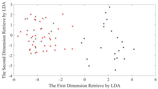
Figure 4. Example of dimensionality reduction.

3.5. Using the Neural Networks to Identify the Status of Machineries

In this section, we discuss the use of neural networks to identify the operating status of machinery. We introduce the structure of the proposed neural network, outline the training equations, and illustrate the process of identifying the operating status. Figure 5 presents the structure of the proposed neural network, which includes three layers: an input layer, a hidden layer, and an output layer. The input layer receives the features selected by the LDA, which are then relayed to the hidden layer. Thus, the number of nodes in this layer must equal the number of selected features. The hidden layer merges the features and then uses a set of activation functions to formulate the relationship between the features and the status of the machinery. Note that in this study, we selected the hyperbolic tangent sigmoid function as an activation function, due to the fact that it features dual polarity signals, which have proven highly effective in neural networks [42]. We opted for two nodes in this layer, based on the recommendation of Chen and Lee [15]. The output layer has only one node, which is responsible for determining the status of the machinery. A value is closer to 1 indicates that the machinery is working well, whereas a value closer to −1 is an indication of abnormal operating status.

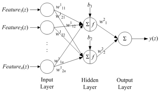
Figure 5. The structure of the proposed neural network.

In the following, we introduce the equations used in the proposed neural network [15]. Equations (8)–(10) are used for the input, hidden, and output layers, respectively. To facilitate this discussion, have also included z to represent the zth set of features.

$$ou{t}_i^{(\mathrm{input}\mathrm{layer})}(z)=inpu{t}_i^{(\mathrm{input}\mathrm{layer})}(z)$$

(8)

$$ou{t}_i^{(\mathrm{hidden}\mathrm{layer})}(z)=\frac{\left(\begin{array}{c}\exp ({\displaystyle \sum _{j=1}^r{w}^1{}_{ij}ou{t}_j^{(\mathrm{input}\mathrm{layer})}(z)+b_i})\\ -\exp (-{\displaystyle \sum _{j=1}^r{w}^1{}_{ij}ou{t}_j^{(\mathrm{input}\mathrm{layer})}(z)+b_i})\end{array}\right)}{\left(\begin{array}{c}\exp ({\displaystyle \sum _{j=1}^r{w}^1{}_{ij}ou{t}_j^{(\mathrm{input}\mathrm{layer})}(z)+b_i})\\ +\exp (-{\displaystyle \sum _{j=1}^r{w}^1{}_{ij}ou{t}_j^{(\mathrm{input}\mathrm{layer})}(z)+b_i})\end{array}\right)}$$

(9)

$$y(z)={\displaystyle \sum _{j=1}^2{w}^2{}_{j}ou{t}_j^{(\mathrm{hidden}\mathrm{layer})}(z)}$$

(10)

From the above equations, we derived the equations for training the neural network based on the concept of back propagation [15]. We first assume that the target function intended for the training network should be as follows:

$$Error(w,z)=\raisebox{1ex}{$1$}\!\left/ \!\raisebox{-1ex}{$2$}\right.{(y_d(z)-y(z))}^2=\raisebox{1ex}{$1$}\!\left/ \!\raisebox{-1ex}{$2$}\right.error{(z)}^2$$

(11)

where error(z) is the error value between the ideal output y_d(z) and actual network output y(z). Based on the theorem of back propagation, all parameter in the neural network can be adjusted using the following function:

$$w(z)=w(z-1)+\xi (-\frac{{\partial }^{+}Error}{\partial w})$$

(12)

where w is used as w¹, b, and w² in Equations (8)–(10), respectively. Thus, we obtain the training functions of this neural network, as follows:

$$w^1(z)=w^1(z-1)+\xi \left[\begin{array}{c}error(z)w^2\times inpu{t}^{(inputlayer)}(z)\times \\ \raisebox{1ex}{$4$}\!\left/ \!\raisebox{-1ex}{${\left(\begin{array}{c}\exp (ou{t}_{}^{(inputlayer)}(z))\\ +\exp (-ou{t}_{}^{(inputlayer)}(z))\end{array}\right)}^2$}\right.\end{array}\right]$$

(13)

$$b(z)=b(z-1)+\xi \left[\begin{array}{c}error(z)w^2\times \\ \raisebox{1ex}{$4$}\!\left/ \!\raisebox{-1ex}{${\left(\begin{array}{c}\exp (ou{t}_{}^{(inputlayer)}(z))\\ +\exp (-ou{t}_{}^{(inputlayer)}(z))\end{array}\right)}^2$}\right.\end{array}\right]$$

(14)

$$w^2(z)=w^2(z-1)+\xi (e\left(z\right)ou{t}_{}^{(hiddenlayer)}(z)),$$

(15)

After training the neural network using Equations (13)–(15), the feature set in input to enable the identification of machinery status. For example, if a signal collected from the machinery can be divided into 100 windows, then these windows are transformed into a set of 100 features. Situations in which the neural network recognizes more than half of these features are identified as abnormal; otherwise, the operating status of the machinery is regarded as normal.

4. Scheduling Algorithms

In the following chapter, we introduce a novel multi-objective scheduling algorithm based on the skyline query for SMEs. To the best of our knowledge, this is the first study to formulate a scheduling algorithm using skyline queries. It should be noted that the proposed scheduling algorithm was developed under the assumption that most of the jobs in smaller enterprises are implemented by single machinery, and that the operation of the machinery is seldom interrupted. Furthermore, for the sake of simplicity, we assumed that each machine in the enterprise is equal with regard to operating efficiency.

Figure 6 presents a flow chart of the proposed scheduling algorithm. For the sake of explanation, let us assume that there are n jobs and m machines (n > m) in this problem, and the maximum delay and the maximum flow time are our only concerns. The algorithm included a heap-based combination pool or the storage of all temporary schedules in the process and a skyline schedule list to store the results of the algorithm. The first step involves obtaining all possible schedules that each machine will be assigned the first job, to be evaluated based on the maximum delay time and maximum flow time. The example in Table 3 includes four jobs (a, b, c, and d) and three machines (A, B, and C).

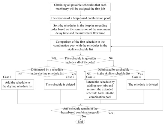
Figure 6. Chart of the proposed scheduling algorithm.

Table 3. Example results obtained from the first step of the proposed scheduling algorithm.

Possible Schedules	Maximum Delay Time	Maximum Flow Time
{A(a), B(b), C(c)}	1 h	3 h
{A(a), B(b), C(d)}	2.5 h	6 h
{A(a), B(c), C(d)}	3 h	5 h
{A(b), B(c), C(d)}	4 h	5.5 h

The second step involves the creation of a heap-based combination pool, wherein all of the schedules obtained in step 2 are sorted in ascending order based on the summation of the maximum delay time and the maximum flow time. This sorting process is used to accelerate the execution speed of the algorithm, based on the fact that objects with a smaller summation value are more likely to be selected as the final result in a skyline query, and should therefore be examined first [14]. Using Table 3 as an example, we obtained the results in Table 4 with all of the schedules arranged according to the summation values of the maximum delay time and the maximum flow time.

Table 4. Example results obtained in the second step of the proposed scheduling algorithm.

Possible Schedules	Maximum Delay Time	Maximum Flow Time	Summation
{A(a), B(b), C(c)}	1 h	3 h	4 h
{A(a), B(c), C(d)}	3 h	5 h	8 h
{A(a), B(b), C(d)}	2.5 h	6 h	8.5 h
{A(b), B(c), C(d)}	4 h	5.5 h	9.5 h

The third step of this algorithm involves a comparison of the first schedule in the combination pool with the schedules in the skyline schedule list. Each comparison can lead to five possible results.

(1) The schedule in question includes all of the jobs and is not dominated by any schedule in the skyline schedule list. In this case, the schedule is deemed a skyline schedule, as it is dominated by no other schedule. It is therefore added to the skyline schedule list, whereupon we return to the third step for further comparisons.

(2) The schedule in question includes all of the jobs and is dominated by a schedule in the skyline schedule list. In this case, the schedule is deemed not to be a skyline schedule, as it is dominated by other schedules. It is therefore immediately deleted from the combination pool, whereupon we return to the third step for further comparisons.

(3) The schedule in question does not include all of the jobs and is not dominated by any schedule in the skyline schedule list. In this case, an extension of the schedule still could still be a skyline schedule. We therefore extend this schedule by adding new jobs and reinsert the extended schedule back into the combination pool, whereupon we return to the third step for further comparisons.

Table 5 presents an example to illustrate this case. If the first schedule {A(a), B(b), C(c)} in the heap is not dominated by any schedule in the skyline list, then we should extend it as{A(a, d), B(b), C(c)}, {A(a), B(b, d), C(c)}, and {A(a), B(b), C(c, d)}. We then evaluate the summation of the maximum delay time and maximum flow time of each schedule and reinsert them back into the heap. Table 4 presents one possible result.

Table 5. Example results obtained in the third step of the proposed scheduling algorithm.

Possible Schedules	Maximum Delay Time	Maximum Flow Time	Summation
{A(a, d), B(b), C(c)}	1 h	3 h	4 h
{A(a), B(c), C(d)}	3 h	5 h	8 h
{A(a), B(b, d), C(c)}	2.1 h	6 h	8.1 h
{A(a), B(b), C(d)}	2.5 h	6 h	8.5 h
{A(a), B(b), C(c, d)}	4.2 h	5 h	9.2 h
{A(b), B(c), C(d)}	4 h	5.5 h	9.5 h

(4) The schedule in question does not include all jobs and is dominated by a schedule in the skyline schedule list. In this case, no extension of the examined schedule could be a skyline schedule. It is immediately deleted from the heap-based combination pool, whereupon we return to the third step for further comparisons.

(5) No schedules remain in the heap-based combination pool. In this situation, all possible schedules have been examined; that is, the scheduling algorithm is completed.

Following the completion of the scheduling algorithm, the schedules remaining in the skyline scheduling list represent the final results.

5. Simulations

In this chapter, we adopt actual data obtained from a small-scale enterprise involved in the manufacture of metal springs to demonstrate the efficacy of the proposed algorithm.

5.1. Experiment Settings

Data were collected from a small Taiwanese enterprise engaged in the manufacture of springs. Most of the springs were meant for export to enterprises in Japan, where the tolerances are particularly low. As a result, the enterprise was eager to obtain assistance in monitoring machinery in order to maintain/improve product quality. Furthermore, this enterprise produces items for more than 50 companies, with new orders coming in every month (many of which are urgent). This greatly complicates scheduling, which often has to be updated several times each day. Clearly, this enterprise requires a systematic method by which to monitor and schedule the use of machinery.

To enable the monitoring of machinery, we employed a three-axis accelerometer (KSM001 ADXL345) with Arduino microcontroller (Uno r3) to collect vibration data from the machinery. This system was applied to a well-worn machine (approximately 10 years old), as shown in Figure 7. This machine was designed based on a cam mechanism mixed with an electrical 3-axis station. Also, this machine offers a Computer Numerical Control (CNC) with an AC servo motor. Metal wire is output from the small hole in the middle of the machine to be shaped into a spring by the surrounding tools. The accelerometer was attached along main axis of the machine, as shown in the middle in Figure 7. All data collect from the Arduino unit was stored in a computer as a Comma-Separated Values (CSV) file to facilitate subsequent processing.

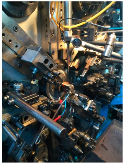
Figure 7. Spring fabrication machine used in experiment.

Scheduling was based on data pertaining to actual orders, which was held in an enterprise database (Table 6). Note that all of these tasks were implemented on a single machine; that is, they were not split up among multiple machines. For the sake of simplicity, we established a set time for scheduling (31 May 2016; 22:00:00). Based on a suggestion from the enterprise workers, we focused only on the maximum delay time and maximum flow time.

Table 6. Jobs for the spring enterprise.

Job	Working Time	Deadline
A	350 min	17 June 2016
B	600 min	23 May 2016
C	300 min	3 June 2016
D	500 min	10 June 2016
E	240 min	6 June 2016
F	230 min	28 May 2016
G	300 min	29 June 2016
H	400 min	30 May 2016
I	240 min	27 May 2016
J	130 min	26 June2016

5.2. Identification of Machinery Status

Table 7 lists the dataset used for training, including 7 spring lengths indicative of normal status and 6 spring lengths indicative of abnormal status. According to an employee in the enterprise, a standard spring should be 191 mm in length, with variations of no more than 2 mm (i.e., between 189 mm and 193 mm). Springs outside this range of error are deemed anomalous. For each category of data, we collected ten signals over a period of 20 s, which is the time required for the fabrication of five springs. We then used the method outlined in Section 3 to identify the status of the machinery, the results of which are listed in Table 8. In this table, we can see that the recognition rate for normal springs is (5 + 6 + 5 + 4)/(10 × 4) = 50%, whereas the recognition rate for normal springsis (7 + 7 + 8 + 6 + 8 + 6 + 7 + 7)/(10 × 8) = 70%. The disappointing recognition rate can be attributed to two problems: (1) the differences between the signals associated with different lengths were too small to be recognized using the sensor; particularly in the range of 187 mm to 195 mm; and (2) the machinery used in this experiment was approximately 10 year old, and therefore produced more vibration-related noise than could be effectively filtered out.

Table 7. Training dataset (Unit of measure: millimeter).

Abnormal	171	181	188	187	195	210	230	194
Normal	189	190	191	192	193

Table 8. Recognition results for springs of all lengths.

Dataset	Identity to Normal	Identity to Abnormal
171	3	7
181	3	7
187	2	8
188	4	6
189	5	5
190	6	4
192	5	5
193	4	6
194	2	8
195	4	6
210	3	7
230	3	7

5.3. Scheduling System

Table 9 lists the time costs obtained using the proposed scheduling algorithm in which ten jobs are divided up between 3 and 5 machines. As shown in the table, the time costs assigned by the algorithm are reduced with the number of machines. This is because an increase in the number of available machines reduces the number of possible schedules, such that fewer schedules need to be checked by the algorithm. Furthermore, reducing the number of possible schedules reduces the maximum delay time and maximum flow time, thereby reducing the number of schedules that eventually become skyline schedules. In other words, the algorithm no longer has to spend an excessive amount of time examining the dominance relationship between the first term of heap and the schedules in the skyline schedule list.

Table 9. Time cost of the proposed scheduling algorithm with 10 jobs.

Number of Machineries	Time Cost
3 machines	18.45 s
4 machines	11.39 s
5 machines	6.22 s

Table 10 lists the results of a comparison between the proposed algorithm and two existing scheduling algorithms: “shortest processing time first plus machinery’s load” (SOT) and “earliest due date first plus machinery’s load” (DDate). The two existing algorithms produced only one answer, rather than the multiple results returned by the proposed algorithm. We considered the following nine cases: 3 machines with 8, 9 or 10 jobs, 4 machines with 8, 9 or 10 jobs, and 5 machines with 8, 9 or 10 jobs. We then used the average results of these nine cases for comparisons. Table 9 clearly illustrates the superiority of the proposed algorithm with regard to maximum flow time as well as maximum delay time. The one exception is the maximum delay time of the DDate, which was designed to minimize the maximum delay time in scheduling problems. No existing algorithm is able to outperform DDate on this point; however, the proposed algorithm was able to match the performance of DDate. This is a clear demonstration that the proposed algorithm is always able to obtain the optimal solution for maximum delay time.

Table 10. Difference between the proposed scheduling algorithm and two existing algorithms.

Other Algorithms	Difference between SOT/DDATE and the Proposed Algorithm: Maximum Flow Time	Percentage Improvement Achieved by the Proposed Algorithm: Maximum Flow Time	Difference between SOT/DDATE and the Proposed Algorithm: Maximum Delay Time	Percentage Improvement Achieved by the Proposed Algorithm: Maximum Delay
SOT	+3.36 h	19.3%	+29.44 h	9.6%
DDATE	+0.81 h	5.55%	0 h	0

5.4. Information Integration

All of the information was uploaded to a web server to provide web page access to the working status of the machinery and scheduled order of all jobs in the queue. Figure 8 presents the interface of the web page. The green bar next to the machines indicates the current working status; that is, green for normal and red for abnormal. The table in the middle lists the job on which the machine is currently engaged, as well as the product quantity, time estimates, and other important data. The table at the bottom lists the schedule including the next job in the queue.

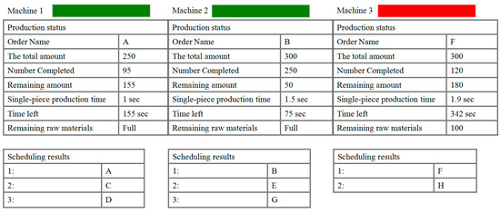
Figure 8. Machine operating data integrated on web page.

6. Conclusions

Since the advent of Industry 4.0, a growing number of manufacturers have been adopting technologies for the monitoring and scheduling of machinery with the aim of increasing yields and optimizing production efficiency. Unfortunately, many of these technological innovations are too expensive for SMEs. In this study, we developed an inexpensive alternative to these two technologies, including add-on sensors by which to monitor the status of machines and a simple algorithm to solve multiple objective scheduling problems. The efficacy of the proposed algorithm was demonstrated in an actual enterprise involved in the manufacture of metal springs. However, our simulation results revealed two limitations of the proposed method: (1) when there is only a small difference between normal and abnormal springs, the use of a low-cost sensor provides disappointing recognition results, due to the low sampling rate and limited accuracy of the sensor; and (2) noise from the monitored machine can also lower the recognition rate, particularly when using a low-cost sensor. In the future, we will investigate the use of multiple low-cost sensors to overcome these problems. It is expected that this will allow the collection of more data that could be used by the algorithm for error recognition. It may also be possible to adopt another algorithm to perform wavelet analysis (i.e., to dismantling the sensor signal) prior to the recognition process. It is very likely that other types of neural network could also be used to enhance recognition performance.

References

- Lee, J.; Kao, H.A.; Yang, S. Service Innovation and Smart Analytics for Industry 4.0 and Big Data Environment. Procedia CIRP 2014, 16, 3–8. [Google Scholar] [CrossRef]
- Lee, J.; Bagheri, B.; Kao, H.A. A Cyber-Physical Systems architecture for Industry 4.0-based manufacturing systems. Manuf. Lett. 2015, 3, 18–23. [Google Scholar] [CrossRef]
- Dassisti, M.; Giovannini, A.; Merla, P.; Chimienti, M.; Panetto, H. An approach to support Industry 4.0 adoption in SME s using a core-meta model. Annu. Rev. Control 2018. [Google Scholar] [CrossRef]
- Uriarte, L.; Azcárate, S.; Herrero, A.; Lopez de Lacalle, L.N.; Lamikiz, A. Mechanistic modeling of the micro end milling operation. J. Eng. Manuf. 2008, 222, 23–33. [Google Scholar] [CrossRef]
- Rivero, A.; Lopez de Lacalle, L.N.; Penalva, M.L. Tool wear detection in dry high-speed milling based upon the analysis of machine internal signals. Mechatronics 2008, 18, 627–633. [Google Scholar] [CrossRef]
- Plapper, V.; Weck, M. Sensor less machine tool condition monitoring based on open NCs. In Proceedings of the IEEE International Conference on Robotics and Automation, Seoul, Korea, 21–26 May 2001; pp. 3104–3108. [Google Scholar]
- Barrio, H.G.; Moran, I.C.; Ealo, J.A.; Barrena, F.S.; Beldarrain, T.O.; Zabaljauregui, M.C.; Zabala, A.M.; Arriola, P.J.A.; Marcaide, L.N.L.L.C. A reliable machining process by means of intensive use of modeling and process monitoring: Approach 2025. Eng. J. DYNA 2018, 93, 689–696. [Google Scholar]
- Birkel, H.S.; Veile, J.W.; Muller, J.M.; Hartmann, E.; Voigt, K.I. Development of a Risk Framework for Industry 4.0 in the Context of Sustainability for Established Manufacturers. Sustainability 2019, 11, 384. [Google Scholar] [CrossRef]
- Moeuf, A.; Pellerin, R.; Lamouri, S.; Tamayo-Giraldo, S.; Barbaray, R. The industrial management of SMEs in the era of Industry 4.0. Int. J. Prod. Res. 2018, 56, 1118–1136. [Google Scholar] [CrossRef]
- Muller, J.M.; Voigt, K.I. Sustainable Industrial Value Creationin SMEs: A Comparison between Industry 4.0 and Made in China 2025. Int. J. Precis. Eng. Manuf.-Green Technol. 2018, 5, 659–670. [Google Scholar] [CrossRef]
- Ivanov, D.; Dolgui, A.; Sokolov, B.; Werner, F.; Ivanova, M. A dynamic model and an algorithm for short-term supply chain scheduling in the smart factory industry 4.0. Int. J. Prod. Res. 2016, 54, 386–402. [Google Scholar] [CrossRef]
- Kyparisis, G.J.; Koulamas, C.P. Flexible Flow Shop Scheduling with Uniform Parallel Machineries. Eur. J. Oper. Res. 2006, 168, 985–997. [Google Scholar] [CrossRef]
- Tahar, D.N.; Yalaoui, F.; Chu, C.; Amodeo, L. A Linear Programming Approach for Identical Parallel Machinery Scheduling with Job Splitting and Sequence-dependent Setup Times. Int. J. Prod. Econ. 2006, 99, 63–73. [Google Scholar] [CrossRef]
- Bartolini, I.; Ciaccia, P.; Patella, M. SaLSa: Computing the skyline without scanning the whole sky. In Proceedings of the 15th ACM International Conference on Information and Knowledge Management, Arlington, VA, USA, 6–11 November 2006; pp. 405–414. [Google Scholar]
- Chen, Y.C.; Lee, C. The σ-Neighborhood Skyline Queries. Inf. Sci. 2015, 322, 92–114. [Google Scholar] [CrossRef]
- Papadias, D.; Tao, Y.; Fu, G.; Seeger, B. An optimal and progressive algorithm for skyline queries. In Proceedings of the 2003 ACM SIGMOD International Conferenceon Management of Data, SanDiego, CA, USA, 9–12 June 2003. [Google Scholar]
- Peng, G.; Jiang, Y.; Xu, J.; Li, X. A Collaborative Manufacturing Execution Platform for Space Product Development. Int. J. Adv. Manuf. Technol. 2012, 62, 443–455. [Google Scholar] [CrossRef]
- Chalal, M.; Boucher, X.; Marques, G. Decision Support System for Servitization of Industrial SMEs: A Modelling and Simulation Approach. J. Decis. Syst. 2015, 24, 355–382. [Google Scholar] [CrossRef]
- Givehchi, M.; Haghighi, A.; Wang, L. Generic Machining Process Sequencing Through a Revised Enriched Machining Feature Concept. J. Manuf. Syst. 2015, 37, 564–575. [Google Scholar] [CrossRef]
- Dombrowski, U.; Ernst, S. Scenario-Based Simulation Approach for Layout Planning. Procedia CIRP 2013, 12, 354–359. [Google Scholar] [CrossRef]
- Denkena, B.; Dengler, B.; Doreth, K.; Krull, C.; Horton, G. Interpretation and Optimization of Material Flow Via System Behavior Reconstruction. Prod. Eng. 2014, 8, 659–668. [Google Scholar] [CrossRef]
- Velandia, D.M.S.; Kaur, N.; Whittow, W.G.; Conway, P.P.; West, A.A. Towards Industrial Internet of Things: Crankshaft Monitoring, Traceability and Tracking Using RFID. Robot. Comput.-Integr. Manuf. 2016, 41, 66–77. [Google Scholar] [CrossRef]
- MacKerron, G.; Kumar, M.; Kumar, V.; Esain, A. Supplier Replenishment Policy Using E-Kanban: A Framework for Successful Implementation. Prod. Plan. Control 2014, 25, 161–175. [Google Scholar] [CrossRef]
- Barenji, A.V.; Barenji, R.V.; Roudi, D.; Hashemipour, M. A Dynamic Multi-Agent-Based Scheduling Approach for SMEs. Int. J. Adv. Manuf. Technol. 2017, 89, 3123–3137. [Google Scholar]
- Yang, J.Y.; Chen, Y.P.; Lee, G.Y.; Liou, S.N.; Wang, J.S. Activity Recognition Using One Triaxial Accelerometer: A Neuro-Fuzzy Classifier with Feature Reduction. Lect. Notes Comput. Sci. 2007, 4740, 395–400. [Google Scholar]
- Abidine, M.; Fergani, B. Evaluating a new classification method using PCA to human activity recognition. In Proceedings of the 2013 International Conference on Computer Medical Applications (ICCMA), Sousse, Tunisia, 20–22 January 2013. [Google Scholar]
- Uray, M.; Skocaj, D.; Roth, P.M.; Bischof, H.; Leonardis, A. Incremental LDA Learning by Combining Reconstructive and Discriminative Approaches. In Proceedings of the British Machinery Vision Conference (BMVC2007), Warwick, UK, 10–13 September 2007. [Google Scholar]
- Ye, J.; Li, Q.; Xiong, H.; Park, H.; Janardan, R.; Kumar, V. IDR/QR: An incremental dimension reduction algorithm via QR decomposition. IEEE Trans. Knowl. Data Eng. 2005, 17, 1208–1222. [Google Scholar]
- Bao, L.; Intille, S.S. Activity recognition from user- annotated acceleration data. In Proceedings of the International Conference on Pervasive Computing, Linzand Vienna, Austria, 21–23 April 2004; pp. 1–17. [Google Scholar]
- Kose, M.; Incel, O.D.; Ersoy, C. Online Human Activity Recognition on Smart Phones. In Proceedings of the Workshop on Mobile Sensing: From Smart phones and Wearables to Big Data, Beijing, China, 16 April 2012. [Google Scholar]
- Chen, Y.C.; Lee, C. A Neural Skyline Filter for Accelerating the Skyline Search Algorithms. Expert Syst. 2015, 32, 108–131. [Google Scholar]
- Karantonis, D.M.; Narayanan, M.R.; Mathie, M.; Lovell, N.H.; Celler, B.G. Implementation of a real-time human movement classifier using a triaxial accelerometer for ambulatory monitoring. IEEE Trans. Inf. Technol. Biomed. 2006, 10, 156–167. [Google Scholar] [CrossRef] [PubMed]
- Kaghyan, S.; Sarukhanyan, H. Activity recognition using K-nearestneighbor algorithm on smart phone with Tri-axialaccelerometer. Inf. Models Anal. 2012, 1, 146–156. [Google Scholar]
- Jatoba, L.; Grossmann, U.; Ottenbacher, J.; Stork, W.; Muller-Glaser, K. Development of a self-constructing neuro-fuzzy inference system for online classification of physical movements. In Proceedings of the 2007 9th International Conference on e-Health Networking, Application and Services, Taipei, Taiwan, 19–22 June 2007; pp. 332–335. [Google Scholar]
- Wang, S.; Yang, J.; Chen, N.; Chen, X.; Zhang, Q. Human activity recognition with user-free accelerometers in the sensor networks. In Proceedings of the IEEE International Conference on Neural Networks and Brain, Beijing, China, 13–15 October 2005; Volume 2, pp. 1212–1217. [Google Scholar]
- Watanabe, T.; Yamagishi, S.; Murakami, H.; Furuse, N.; Hoshimiya, N. Recognition of lower limb movements by artificial neural network for restoring gait of Hemiplegic patients by functional electrical stimulation. In Proceedings of the IEEE International Conferenceon Engineering in Medicine and Biology Society, Istanbul, Turkey, 25–28 October 2001; pp. 1348–1351. [Google Scholar]
- Blazewicz, J.; Dror, M.; Weglarz, J. Mathematical Programming Formulations for Machinery Scheduling: A Survey. Eur. J. Oper. Res. 1991, 51, 283–300. [Google Scholar]
- Lauff, V.; Werner, F. On the Complexity and Some Properties of Multi-stage Scheduling Problems with Earliness and Tardiness Penalties. Comput. Oper. Res. 2004, 31, 317–345. [Google Scholar]
- Borzsonyi, S.; Kossmann, D.; Stocker, K. The skyline operator. In Proceedings of the 17th International Conference on Data Engineering, Heidelberg, Germany, 2–6 April 2001; pp. 235–254. [Google Scholar]
- Nawaz, J.M.; Arshad, M.Z.; Hong, S.J. Time Series Fault Prediction in Semiconductor Equipment Using Recurrent Neural Network. In Proceedings of the International Symposium on Neural Networks, Dalian, China, 4–6 July 2013; pp. 463–472. [Google Scholar]
- Shao, Y.; Li, X.; Mechefske, C.K.; Zuo, M.J. Use of Neural Networks to Predict Rear Axle Gear Damage. In Proceedings of the International Conference on Reliability, Maintainability and Safety, Chengdu, China, 20–24 July 2009; pp. 986–990. [Google Scholar]
- Wang, J.S.; Chen, Y.C. A Hammerstein- Wiener recurrent neural network with universal approximation capability. In Proceedings of the IEEE International Conference on Systems, Man and Cybernetics, Singapore, 12–15 October 2008; pp. 1832–1837. [Google Scholar]
© 2019 by the authors. Licensee MDPI, Basel, Switzerland. This article is an open access article distributed under the terms and conditions of the Creative Commons Attribution (CC BY) license (http://creativecommons.org/licenses/by/4.0/).