Article

An Electric Load Simulator for Engine Camless Valvetrains

School of Mechanical Engineering, Nanjing University of Science and Technology, Nanjing 210094, China
*
Author to whom correspondence should be addressed.
Appl. Sci. 2019, 9(8), 1591; https://doi.org/10.3390/app9081591
Submission received: 19 January 2019 / Revised: 1 April 2019 / Accepted: 15 April 2019 / Published: 17 April 2019
(This article belongs to the Section Mechanical Engineering)

Abstract

:
Camless valvetrains have become a promising direction to improve the performance of internal combustion engines. In this paper, an electric load simulator is proposed to simulate and implement gas force on the exhaust valve for camless valvetrains under semi-physical conditions. According to test data, the 1D gas-dynamic model was established to get boundary conditions and initial values for 3D finite element simulation. The 3D finite element simulation model was solved to obtain the gas force characteristics of the exhaust valve for camless valvetrains. The electromagnetic actuator was designed according to the system scheme and performance requirements of the electric load simulator. The PID (Proportion Integration Differentiation) algorithm was designed to control the output force of the electric load simulator and reproduce the gas force characteristics of the exhaust valve. It was found that the output force of the electric load simulator could follow the variation of the target gas force and meet the performance requirements of the electric load simulator based on simulation results and experimental results.

1. Introduction

The conventional valvetrains with camshafts use fixed cam profiles to get a reasonable compromise between speed stability, fuel economy, and torque performance. However, cam-driven valvetrains do not have efficiencies as large as camless valvetrains over a wide range of engine operation [1]. Camless valvetrains can achieve variable valve timing and opening duration by controlling individual valves. Therefore, in the face of increasingly scarce oil resources and serious environmental problems, studies on camless valvetrains have important research significance to improve the power and economy of automobiles and to reduce energy consumption and pollutant emissions [2].
During the engine exhaust stroke, there is a large pressure difference between the cylinder and exhaust passage when the exhaust valve starts to open. Under these circumstances, the exhaust valve is subjected to large gas force. Depending on the operating conditions of the engine, the combustion pressure in the combustion chamber changes between 0 and 7 bar when the exhaust valve begins to open [3]. Once the exhaust valve is opened, the exhaust gas flows out of the combustion chamber, and the pressure difference between the upper and lower end faces of the exhaust valve is gradually released [4]. As the exhaust valve opens, the gas force tends to decrease to zero gradually from a higher initial value [5].
Junfeng Zhao and other scholars from the University of British Columbia in Canada conducted research on gas force. For a typical valve with a diameter of 25 mm, the initial pressure during the exhaust stroke is 5 bar, and the initial gas force acting on the valve is 250 N. Ryan R. Chladny and other scholars at the University of Alberta in Canada proposed that the energy lost by gas force is roughly the product of the valve lift and half of the initial force. Therefore, the gas force with an initial value of 250 N will dissipate 1 J of energy loss at a valve lift of 8 mm, which will dissipate half of the available potential energy during valve motion [3,4,5]. On the other hand, the gas force has a large influence on the trajectory and small contact velocity of the valve. The small contact velocity is correlated with noise and increased component wear, which is difficult to achieve under real operating conditions depending on various engine speeds and loads, as well as unknown gas forces acting on the valves [6,7,8,9].
In order to test the static performance and dynamic characteristics of the camless valvetrains under load, to save research costs, and to shorten development cycle, it is necessary to carry out simulation and experimental research to reproduce the actual gas force of the valve. Two methods are generally available: physical test and semi-physical test. In the physical test, the engine needs to be burned and work. The stability of the control system is evaluated by actual measurements. This method requires much material, human, and financial resource, so it is difficult to collect the test data. The semi-physical test can simulate the performance of the valve under load by adopting the load simulator to reproduce gas force and load it onto the valve without the engine burning and working. This method can save research and development cost and improve test reliable. It turns destructive experiments into predictive studies under laboratory conditions and helps researchers foresee and detect the problems that occur in the mechanism and control system before they actually operate [10,11,12,13].
Sang Yeal Lee and Hyung Suck Cho adopted the electro-hydraulic load simulator to generate desired torque profiles. A novel fuzzy logic controller was proposed to improve the transient performance and robustness of the load simulator control system. Simulation and experimental results showed that the load simulator could get faster and more accurate dynamic responses by using the designed controller, compared with the fixed fuzzy controller when the operating point and external disturbances were changed [14].
Considering that the electro-hydraulic torque servo system has some disadvantages, such as nonlinearity and time-variable parameters, high cost, and bulkiness, Xingjian Wang selected the electric load simulator to reproduce load force. The velocity-loop compensation based on improved fuzzy control and combined with PID control through the exponential function was proposed to eliminate extraneous torque. Experimental results showed that the extraneous torque eliminated ratio could reach 92.2% [15]. However, there are many nonlinear factors in the actual system operation, including mechanical friction and structural clearance, which make it impossible to completely eliminate the interference of extraneous torque.
Kang Chen designed an electric load simulator for a linear rudder. The load system used permanent magnet direct current actuators to provide aerodynamic force for the linear servo rudder. PID with forward feed control was used to eliminate the extraneous force. Simulation and experimental results demonstrated that the closed system had less than 5% error between the target force and feedback force. The load system had good tracking performance [16].
In order to study the influence of gas force on the exhaust valve and promote further developments and practical application of camless valvetrains, this paper mainly researches the gas force characteristics of the exhaust valve during engine exhaust stroke and designs the load simulator to simulate the load force under semi-physical conditions. In this paper, we propose a 3D engine model for finite element simulation to obtain gas force characteristics in the exhaust stroke. The system scheme and control strategy of the electric load simulator are designed to reproduce ideal gas force on the exhaust valve. Simulation and experimental results verify that the proposed electric load simulator has satisfactory dynamic performance and stability. The main work is organized as follows. Load characteristics of the exhaust valve for camless valvetrains are presented in Section 2. Section 3 presents the configuration and performance requirements of the electric load simulator. Section 4 proposes the mathematical model of the electric load simulator, which is verified by a computer-controlled experimental test bench. Section 5 analyzes the simulation results and the experimental results of the electric load simulator and discusses the application of the designed load system. Section 6 summarizes the whole work and contributions of this paper.

2. System Design

2.1. System Configurations

The target force that the electric load simulator is required to reproduce is not very large, but the requirements of the bandwidth and accuracy are very high. On the other hand, the bearing object is the exhaust valve, which has a certain motion curve, the load simulator needs to follow the valve passively for linear motion. Therefore, the electric load linear simulator was selected as the load device to implement gas force on the exhaust valve under semi-physical conditions by comparing the advantages and disadvantages of different load simulators, as shown in Table 1 [17,18,19,20].
The schematic diagram of the electric load simulator is shown in Figure 1. It was mainly composed of an electromagnetic actuator, a force sensor, an exhaust valve, a DSP controller, and a control computer. The exhaust valve was the carrying object. It was subjected to electromagnetic force F m a g , spring force F s , damping force F c , inertial force F a , and gas force F g during the exhaust stroke. It was coaxially coupled to the electromagnetic actuator and the force sensor through the connecting shaft. The force sensor was connected with the electromagnetic actuator and exhaust valve by a bolt to measure the output force of the electromagnetic actuator. The concentricity of the force sensor, electromagnetic actuator, and exhaust valve was consistent to transmit the same displacement, speed, and force.
The electromagnetic actuator was used to simulate gas force F g of the exhaust valve. When the exhaust valve moved in a certain displacement curve, the electromagnetic actuator followed the exhaust valve passively through the connecting shaft to achieve passive follow-up of the displacement. At the same time, the electromagnetic actuator simulated the gas force and loaded it onto the exhaust valve to realize the closed-loop control of the output force through the force sensor.
The control system requires high precision and fast response time to ensure the load simulator can reproduce gas force characteristics while moving with the exhaust valve. Since the DSP (Digital Signal Processing) controller has powerful digital signal processing capabilities, relatively complete event management capabilities, and embedded control functions, it is widely used in industrial control. Therefore, DSP was adopted as the core processor of the electric load simulator to use its rich peripheral design control system and powerful arithmetic processing capability. The signal processor and DSP controller were used to handle and convert signals to the control computer for further data analysis and to realize the control of output force.

2.2. Performance Requirements

The main technical requirements of the electric load simulator are listed below according to the technical parameters of the engine [21]:
(1) In view of the fact that the pressure difference between the cylinder and the exhaust port could reach 8 bar during the exhaust stroke, the output force of the electromagnetic actuator should range from 0–320 N to simulate the gas force.
(2) The maximum velocity of the exhaust valve changes from 2 m/s–3 m/s, so the power of the electric load simulator followed: P 960   W .
(3) Bandwidth: ≥ 80 Hz.
(4) The maximum stroke of the electric load simulator: 8–10 mm.
(5) In order to improve the control accuracy of the system, static load accuracy requirements: ≤2% FSR (Full Scale Range), dynamic load accuracy requirements: ≤5% FSR.
(6) Taking the performance and cost of electronic components and other factors into account to meet the system response performance, the system supply voltage followed: U 30   V .

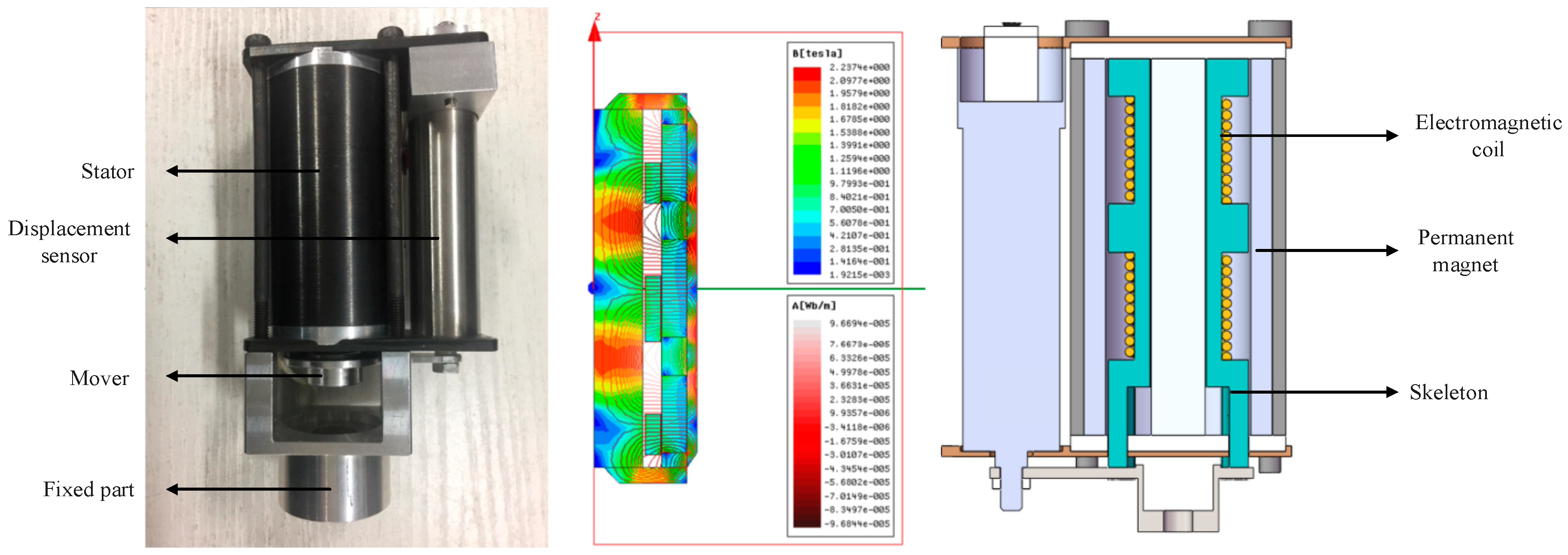
2.3. Electromagnetic Actuator Design

An electromagnetic actuator was designed to reproduce the gas force in view of the configurations and technical requirements of the electric load simulator. It was mainly made up of the mover, stator, displacement sensor, and the fixed part. The prototype and magnetic fluxes of the electromagnetic actuator are shown in Figure 2. The mover and the output shaft of the electromagnetic actuator were connected, which are moving parts. The stator and fixed part were connected. One side of the connection plate of the displacement sensor was pressed and fixed on the mover through the output shaft of the electromagnetic actuator. The other side was screwed with the inner core of the displacement sensor. The mover of the electromagnetic actuator followed the movement of the exhaust valve. Therefore, the speed and displacement signals of the mover could be measured and transmitted to the displacement sensor.
It can be seen from the magnetic fluxes of the electromagnetic actuator that the magnetic lines were densely, evenly, and basically symmetrically distributed after energization. It was less affected by the current. The magnetic induction intensity at the intermediate position of the permanent magnet was the smallest, and the numerical value was approximately zero. The magnetic induction intensity at the intermediate position of the two sets of permanent magnets was the largest, and the numerical value was about 2.24 T [1,22]. The structural parameters of the electromagnetic actuator are shown in Table 2.
The characteristic curve of electromagnetic force is shown in Figure 3. The range of electromagnetic force was from −300 N–300 N, and the magnitude of electromagnetic force was related to coil current and position.

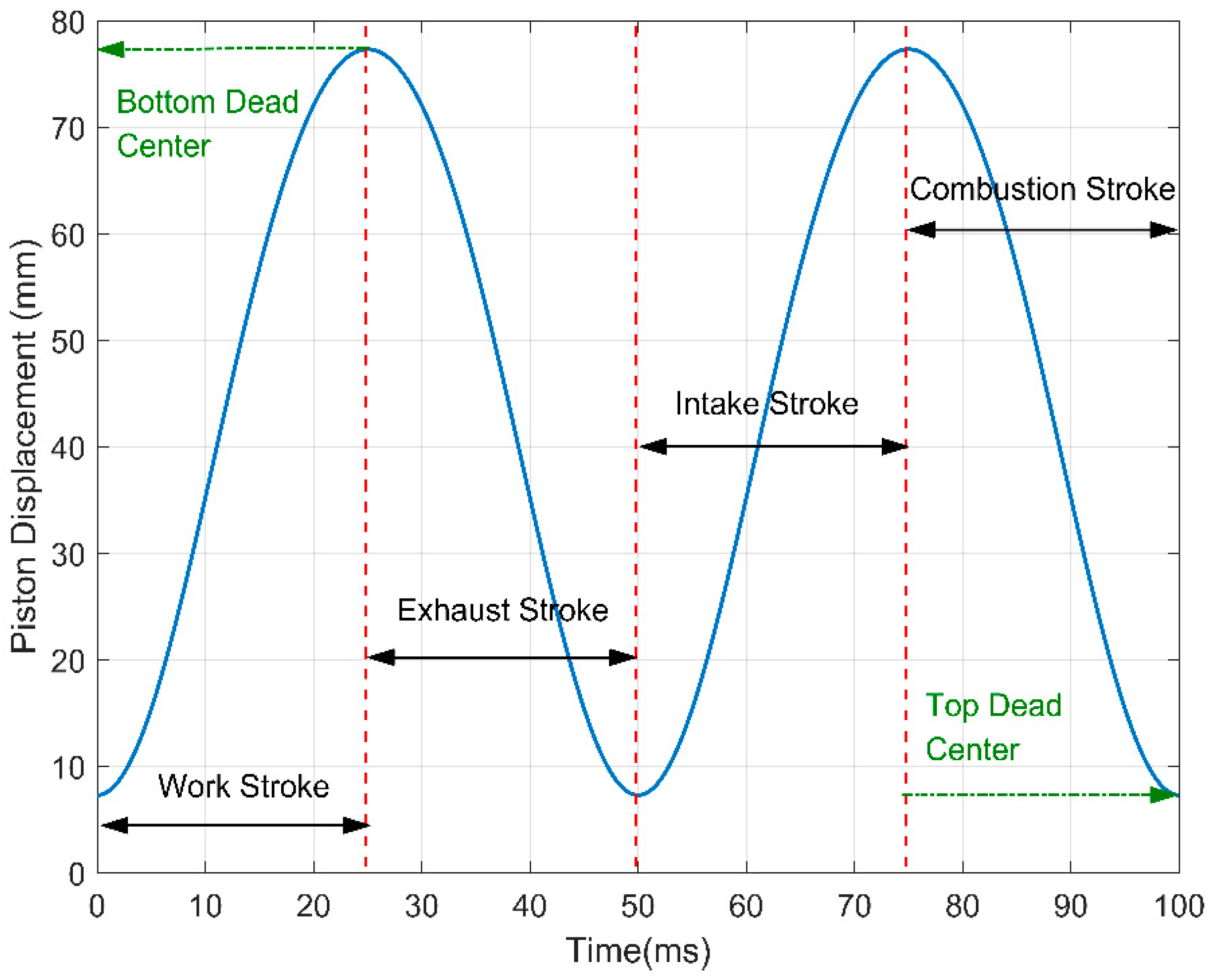
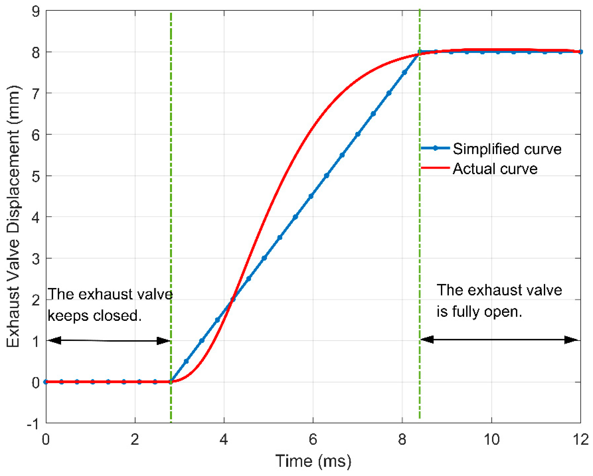
3. Load Characteristics of the Exhaust Valve

3.1. 1D Gas-Dynamic Simulation

In the 3D solution process, the boundary conditions and initial values of the model need to be set. The initial temperature and pressure of the inlet, outlet, combustion chamber, and exhaust passage need to be set in detail so that the in-cylinder simulation environment can be close to the actual working situation at the beginning of the simulation. In order to obtain the boundary and initial values for 3D simulation that are close to the actual working conditions, the 1D simulation model of the engine was established.
Referring to the combustion exothermic law equation of the Vibe model and the Woschni 1978 heat transfer function, which are shown in Equations (1)–(2), the 1D simulation model of the engine was established. The simulation results of the established 1D model were compared with the test data of the prototype machine to revise and adjust model parameters constantly. The 1D gas-dynamic model of the engine is constructed in Figure 4. It mainly consisted of the inlet system, combustion system, and exhaust system [23].
d x d α = α Δ α c ( m + 1 ) y m e a y ( m + 1 ) d x = d Q Q y = α α 0 Δ α c
where x is the percentage of fuel; Q is the total heat release of the fuel injection; α is the crank angle; α 0 is the burning start angle; Δ α c is the combustion duration; m is the shape parameter; a is the Vibe parameter ( a = 6.9 means complete combustion).
α w = 130 D 0.2 P c 0.8 T c 0.53 × [ C 1 C m + C 2 V D T C 1 P C 1 V C 1 ( P C P C 0 ) ] 0.8
where D is cylinder diameter; P c is engine cylinder pressure; T c is engine cylinder temperature; V D is volume per cylinder; P C 0 is cylinder pressure when the engine starts; T C 1 is the cylinder temperature when the intake valve is closed; P C 1 is the cylinder pressure when the intake valve is closed.
1D simulation provides transient boundary conditions and initial values for 3D simulation and enables the accurate solution of the 3D numerical simulation. Since only the exhaust stroke of the engine was considered, the intake valve in the 3D engine model was always closed. The simulation values at Test Points 5 and 6 were used as the initial conditions of cylinder and exhaust passage in the 3D simulation, respectively, as shown in Table 3. The settings of the initial conditions have a large influence on the convergence of the calculation while solving 3D CFD simulation.

3.2. 3D Numerical Simulation

The 3D engine model was established for numerical simulation, which included the cylinder, piston, exhaust valve, and exhaust port, as shown in Figure 5a. The specific technical parameters of the engine are shown in Table 4.
The intake port was always closed because only the exhaust stroke of the engine was considered. In the process of dividing the grid, the exhaust valve and piston were set to move to simulate the actual exhaust stroke of camless valvetrains. The refined regions of the moving parts are shown in Figure 5b.
The operating mode of the engine had four strokes, which included the work stroke, exhaust stroke, intake stroke, and compression stroke. The displacement curve of the piston is shown in Figure 6. The exhaust stroke of the 3D engine model was simulated to obtain the gas force characteristics of the exhaust valve. The piston moved from the bottom dead center to the top dead center.
In the camless engine model, the valve and valve actuator were coupled to each other. The valve actuator drove the valve to move. By controlling the movement of the valve actuator, it is possible to control the displacement curve of the valve. In order to improve the division accuracy and solution speed of the moving mesh, the displacement curve was simplified. The actual curve and simplified curve of the valve actuator during the exhaust stroke are shown in Figure 7. The maximum displacement of the valve was set to 8 mm, and the transition time was 5.76 ms when the exhaust valve was fully open. The exhaust stroke piston moves for 25 ms in Figure 6. The process from closing to full opening of the exhaust valve was 5.76 ms. We mainly studied the gas physical force during the process from opening to full opening of the valve, during which the gas physical force will constantly change due to the change of displacement, which is our research content.
In the process of setting solution conditions, the fluid properties were set to air. The transport equation for the standard k ε wall function was set as Equations (3)–(4) to optimize the laminar flow area.
t ( ρ k ) + x i ( ρ k u i ) = x j [ ( μ + μ i σ k ) k x j ] + G k + G b ρ ε Y M + S K
t ( ρ ε ) + x i ( ρ ε u i ) = x j [ ( μ + μ i σ ε ) ε x j ] + C 1 ε ε k ( G k + C 3 ε G b ) C 2 ε ρ ε 2 k + S ε
where k is turbulent kinetic energy; ε is the dissipation rate; G k is turbulent kinetic energy generated by the average velocity gradient; G b is turbulent kinetic energy generated by buoyancy; Y M is the expansion dissipation rate; C 1 ε , C 2 ε , and C 3 ε are constants; σ k , σ ε are the turbulent Prandtl number of k and of ε ; S K , S ε are user-defined source terms.
Set the turbulent and turbulent energy lengths of the system according to Equations (5)–(7).
Turb . kin . energy = 1.5 * ( u 2 )
Turb . length . scale = H / 2
u = 1.4 * h * ( n / 60 )
where n is engine speed; H is the maximum valve lift; h is the piston stroke.
The values of low relaxation factors, including momentum, pressure, turbulent kinetic energy, and dissipation rate were set as appropriate values to control the speed of the fluid equation and improve the stability of the calculation. A simple algorithm was set to solve the model because it had a large effect on pressure-velocity coupling [24].
The 3D model of the engine was numerically solved based on the 3D numerical simulation software to obtain 2D average results and 3D results. The 3D numerical simulation was started to be solved before the exhaust valve opened in order to create an exhaust environment and observe the changes of parameters in the cylinder and exhaust valve. Based on the 2D average results, the in-cylinder pressure of the 3D simulation was plotted and compared with experimental results. The comparison chart is shown in Figure 8. It can be seen from the comparison chart that the results of 3D numerical simulation were consistent with the changes of the experimental curve. The engine cylinder pressure test result was that the cylinder pressure sensor was placed in the engine to measure the cylinder pressure along with the engine running. At the same crank angle, the maximum relative deviation of the in-cylinder pressure was 4.3%, which verified the accuracy of the 3D simulation model. It is feasible to study gas force characteristics by using the 3D model in further studies.
The area and pressure of each refined region can be obtained on the basis of surface slices and 3D simulation results. The integral method was used to calculate the gas force of the exhaust valve during the exhaust stroke according to Equation (8).
F = P i × A i × cos α i P j × A j × cos α j , i = 1 , 2 ; j = 3 , , 10
where P and A represent the pressure and area of each refined part, respectively; α is the angle between the refined plane and horizontal plane; subscripts i and j refer to the refined regions. The force acting on each refined region and the total gas force of the exhaust valve are shown in Figure 9. The force acting on Regions 8, 9, and 10 was zero because these regions were vertical to the horizontal plane in the movement direction of the exhaust valve.

4. Development and Validation of the System Model

4.1. Mathematical Model of the System

Assuming that eddy currents and magnetic saturation are ignored, there was no gas force acting on the actuator, according to the differential equation of motion, the voltage balance equation, and the electromagnetic force equation of the electromagnetic actuator, the differential equations of the system can be deduced as Equation (9) [25]:
{ I = R L I k m L v + u L v ˙ = k m m I c m v S ˙ = v
where k m and m are the force constant and mass of the electromagnetic actuator; c is the damping coefficient; S and v represent the displacement and velocity; I is the current in the coil; R and L are the coil resistance and coil inductance.
Equation (9) shows that when the system inputs voltage v , coils generate current I . Then, coils with current suffer the electromagnetic force F m a g in the air gap magnetic field. The electromagnetic force drives the electromagnetic actuator. The movement of the electromagnetic actuator generates displacement S and velocity v , which change the value of the electromagnetic force in the form of back-EMF (Electromotive Force). The force constant and the velocity of the electromagnetic actuator will affect the value of current in turn. Therefore, the electromagnetic actuator needs to consider the relationship among various subsystems fully to build an accurate mathematical model.
The PID control algorithm is widely used in industrial control due to its advantages of being a simple algorithm, good robustness, high tracking accuracy, and reliability. Furthermore, it is suitable for a system that has uncertain parameters. Considering that the electric load simulator needs to follow the exhaust valve passively, the PID controller was selected as the control algorithm of the electric load simulator [5,25], which can be described as Equation (10).
U ( s ) = K p ( 1 + 1 T i s + T d s ) E ( s )

4.2. Model Validation

The simulation model of the electric load simulator was mainly composed of the drive actuator, the controller, the power drive module, and the load actuator, as shown in Figure 10. The drive actuator and the load actuator were both composed of the electromagnetic linear actuator, so the simulation model of the electromagnetic actuator module was set up according to the differential Equation (9). The power driver module had the transfer function as K s T s s + 1 , which can be considered as an inertial component. In the function, K s is the amplification factor of the power driver and T s is the lag time constant. The PID controller module was setup according to the transfer function Equation (10).
The drive actuator was used to simulate the displacement curve of the exhaust valve. Since the drive actuator is tightly coupled with the load actuator in actual operations, the load actuator passively followed the motion of the drive actuator. The target load force was set as the gas force obtained from 3D CFD (Computational Fluid Dynamics) simulation. The load actuator was used to simulate gas force while following the movement of the drive actuator under the control of the PID strategy.
In order to verify the accuracy of the mathematical model, the test platform was built to obtain the displacement and current values of the load actuator. The test bench included the electromagnetic actuator, displacement sensor, DSP controller, and control computer. Input 6 V voltage to the electromagnetic actuator at 10 ms, then the current and displacement signals can be obtained from the DSP controller and the control computer.
The experimental results of the load actuator were compared with the simulation results of the load actuator, as shown in Figure 11. It can be concluded from the comparison chart that the trends of the simulation results and experimental results were consistent. Considering that the load actuator should follow the motion of the drive actuator, the movement of the load actuator was set to be the same as the displacement curve of experimental results during simulation. The error of current between simulation results and experimental results was kept below 0.8 A, and the dynamic load accuracy was less than 5% FSR, which meets the system requirements. It was verified that the mathematical model can be used in the following research. In some ways, the errors of experimental results were due to the vibration of the test bench.

5. Results and Discussion

5.1. Simulation Results

The linear response module was used to plot the force response Bode plot of the actuator system, as shown in Figure 12. By analyzing the amplitude-frequency characteristics and phase-frequency characteristics of the simulation results, the amplitude dropped to −3 dB at 330.1 Hz, and the phase difference lagged 90° at 1032 Hz. Therefore, the bandwidth of the system should be 330.1 Hz.
The control parameters of the PID controller were continuously adjusted so that the output force of the load actuator could be changed with the target load force, where K p = 0.05 , K i = 255 , K d = 2 e 6 . In the adjustment process, the role of the proportional link was to scale up the system deviation, so that the deviation of the system changed to the direction of reduction at a faster speed, increased the proportional coefficient to adjust the speed, and reduced the steady-state error. The function of the integral link was to eliminate the steady-state error, so that the actual output value of the system could track the set value without the static difference in the steady-state condition. The appropriate size of the integral time constant can improve the system without any difference. Increasing the differential time constant is helpful to reduce the system adjustment time. Through the comprehensive adjustment of three links, namely the proportional link, integral link, and differential link, the appropriate control parameters were selected to reduce the steady-state error of the system and overcome the overshoot problem of the system, so as to improve the stability of the system and accelerate the dynamic response of the system [26,27].
In the exhaust stroke, the target force that the load actuator needed to output changed from 0–310 N. The comparison chart of the simulation results and target force is shown in Figure 13. It shows that the rise time, peak time, and overshoot of the electric load simulator were 0.12 ms, 0.3 ms, and 19.85%, respectively. The output force of the simulation model ranged from 0–313 N, and changed rapidly at 3.5 ms when the exhaust valve opened 12.5%. During the opening process of the exhaust valve, the error between the output force and target force was kept below 3% FSR. The dynamic load accuracy was kept below 2% FSR after 3.8 ms. Simulation results showed that the output force of the electric load simulator could follow the variation of the target force and meet the requirements of the electric load simulator.

5.2. Experimental Results

The test platform was established to test system performance, which is shown in Figure 14. The platform was made up of the control computer, load actuator, drive actuator, displacement sensor, force sensor, power supply, charge amplifier, and DSP controller. The control computer received signals from DSP controller and monitored the operations of the electric load simulator in real time. DSP controller collected feedback signals of the sensors, output PWM (Pulse Width Modulation) control signals, and realized the operation of the control algorithm. The power drive circuit adjusted the voltage of the load actuator according to the PWM signals. Then, the current in the actuator coil was controlled to achieve the control requirements.
The output force of the electric load simulator should reproduce the target force by adjusting the control parameters of the PID controller continuously. The comparison chart of the experimental results and target force is shown in Figure 13. The rise time, peak time, and overshoot of the electric load simulator were 0.9 ms, 1.1 ms, and 24.5%, respectively. The output force of the electric load simulator ranged from 0–308 N. During the opening process of the exhaust valve, the error between the output force and target force was kept below 5% FSR. The dynamic load accuracy was kept below 2% FSR after 5 ms. Experimental results showed that the output force of the electric load simulator could follow the variation of the target force and meet the requirements of the dynamic load accuracy. Compared with the simulation results, the response of the experimental force had a delay of 1 ms. This was mainly caused by the disturbance of current and displacement to the output force in the actual actuator system.

6. Conclusions

In this paper, the 1D gas-dynamic model and 3D CFD model were established to obtain the gas force that the exhaust valve suffers during the exhaust stroke. An electric load simulator was designed for engine camless valvetrains to exert the gas force on the exhaust valve. The test platform was established to verify the feasibility of mathematical model and test the performance parameters of the electric load simulator. Simulation results and experimental results proved that the electric load simulator had high efficiency, strong robustness, and satisfactory loading performance.
In further research, the electric load simulator can be coupled with the exhaust valve in the camless valvetrains under laboratory conditions to simulate gas force and test the robustness of the control strategy. The influence of gas force on the performance of engines can be tested through semi-physical experiments, which are of great help to anticipate problems in advance and reduce the research cycle.

Author Contributions

Supervision, L.L. and Z.X.; writing, original draft, L.Z.; writing, review and editing, L.Z. and X.Z.

Funding

This work was supported by the National Natural Science Foundation of China (Grant No. 51875290) and Shanghai Aerospace Science and Technology Innovation Fund (SAST2018-107).

Conflicts of Interest

The authors declare no conflict of interest.

References

  1. Ha, K.P.; Han, D.; Kim, W.T. Development of Continuously Variable Valve Lift Engine; SAE Technical Paper; SAE: Warrendale, PA, USA, 2010. [Google Scholar]
  2. Liu, L.; Chang, S. Improvement of valve seating performance of engine’s electromagnetic valvetrain. Mechatronics 2011, 21, 1234–1238. [Google Scholar] [CrossRef]
  3. Zhao, J.; Seethaler, R.J. Compensating combustion forces for automotive electromagnetic valves. Mechatronics 2010, 20, 433–441. [Google Scholar] [CrossRef]
  4. Chladny, R.R.; Koch, C.R. Flatness-Based Tracking of an Electromechanical Variable Valve Timing Actuator with Disturbance Observer Feedforward Compensation. IEEE Trans. Control Syst. Technol. 2008, 16, 652–663. [Google Scholar] [CrossRef]
  5. Schernus, C.; Van Der Staay, F.; Janssen, H.; Neumeister, J.; Vogt, B.; Donee, L.; Estlimbaum, I.; Nicole, E.; Maerky, C. Modeling of Exhaust Valve Opening in a Camless Engine; SAE Technical Paper; SAE: Warrendale, PA, USA, 2002. [Google Scholar]
  6. Haskara, I.; Kokotovic, V.V.; Mianzo, L.A. Control of an electro-mechanical valve actuator for a camless engine. Int. J. Robust Nonlinear Control 2004, 14, 561–579. [Google Scholar] [CrossRef]
  7. Hoffmann, W.; Peterson, K.; Stefanopoulou, A.G. Iterative Learning Control for Soft Landing of Electromechanical Valve Actuator in Camless Engines. Control Syst. Technol. IEEE Trans. 2003, 11, 174–184. [Google Scholar] [CrossRef]
  8. Peterson, K.S.; Stefanopoulou, A.G. Extremum seeking control for soft landing of an electromechanical valve actuator. Automatica 2004, 40, 1063–1069. [Google Scholar] [CrossRef]
  9. Gray, J.; Krstic, N.; Chaturvedi, J. Parameter Identification for Electrohydraulic Valvetrain Systems. J. Dyn. Syst. Meas. Control 2011, 133, 064502. [Google Scholar] [CrossRef]
  10. Yang, B.; Bao, R.; Han, H. Robust Hybrid Control Based on PD and Novel CMAC with Improved Architecture and Learning Scheme for Electric Load Simulator. IEEE Trans. Ind. Electron. 2014, 61, 5271–5279. [Google Scholar] [CrossRef]
  11. Zhao, J.; Shen, G.; Zhu, W.; Yang, C.; Yao, J. Robust force control with a feed-forward inverse model controller for electro-hydraulic control loading systems of flight simulators. Mechatronics 2016, 38, 42–53. [Google Scholar] [CrossRef]
  12. Yang, B.; Bao, R.; Zhang, M.; Wei, Q. A KCMAC-PD controller with reduced memory and optimized mapping for the torque control of electric load simulator. Trans. Inst. Meas. Control 2017. [Google Scholar] [CrossRef]
  13. Truong, D.Q.; Ahn, K.K. Force control for hydraulic load simulator using self-tuning grey predictor—fuzzy PID. Mechatronics 2009, 19, 233–246. [Google Scholar] [CrossRef]
  14. Lee, S.Y.; Cho, H.S. A fuzzy controller for an aero-load simulator using phase plane method. IEEE Trans. Control Syst. Technol. 2001, 9, 791–801. [Google Scholar] [CrossRef]
  15. Wang, X.; Wang, S. High performance torque controller design for electric load simulator. In Proceedings of the 2011 6th IEEE Conference on Industrial Electronics and Applications, Beijing, China, 21–23 June 2011. [Google Scholar] [CrossRef]
  16. Chen, K.; Wang, J.; Yan, J.; Huang, Y. Experiment and study of electric loading simulator for linear rudder. In Proceedings of the IEEE 2008 7th World Congress on Intelligent Control and Automation, Chongqing, China, 25–27 June 2008. [Google Scholar] [CrossRef]
  17. Han, S.; Jiao, Z.; Yao, J.; Shang, Y. Compound Velocity Synchronizing Control Strategy for Electro-Hydraulic Load Simulator and Its Engineering Application. J. Dyn. Syst. Meas. Control 2014. [Google Scholar] [CrossRef] [PubMed]
  18. Basic, G. Hardware-In-The-Loop Simulation of Mechanical Loads for Mechatronics System Design. Ph.D. Thesis, University of Ottawa, Ottawa, ON, Canada, 2003; doi:10393/26323. [Google Scholar]
  19. Wang, C.; Jiao, Z.; Quan, L. Adaptive velocity synchronization compound control of electro-hydraulic load simulator. Aerosp. Sci. Technol. 2015, 42, 309–321. [Google Scholar] [CrossRef]
  20. Olaru, R.; Arcire, A.; Petrescu, C.; Mihai, M. A novel vibration actuator based on active magnetic spring. Sens. Actuators A Phys. 2017, 264, 11–17. [Google Scholar] [CrossRef]
  21. Kim, H.; Son, J.; Lee, J. A High-Speed Sliding-Mode Observer for the Sensor-less Speed Control of a PMSM. IEEE Trans. Ind. Electron. 2011, 58, 4069–4077. [Google Scholar] [CrossRef]
  22. Hanson, B.; Levesley, M. Self-sensing applications for electromagnetic actuators. Sens. Actuators A Phys. 2004, 116, 345–351. [Google Scholar] [CrossRef]
  23. Hota, R.; Munjal, M.; Mukherjee, N. Evaluation of Engine Acoustic Source Characteristics Using AVL BOOST Software; Mechanical Engineering: Cambridge, MA, USA, 2008. [Google Scholar]
  24. Baburic, M.; Željko, B.; Neven, D. A New Approach to CFD Research: Combining AVL’s Fire Code with User Combustion Model. In Proceedings of the International Conference Information Technology Interfaces, Cavtat, Croatia, 24–27 June 2002. [Google Scholar] [CrossRef]
  25. Lesan, W.; Mingyan, W.; Ben, G.; Zhe, W.; Di, W.; Yanlin, L. Analysis and Design of a Speed Controller for Electric Load Simulators. IEEE Trans. Ind. Electron. 2016, 63, 7413–7422. [Google Scholar] [CrossRef]
  26. Mercorelli, P.; Werner, N. An Adaptive Resonance Regulator Design for Motion Control of Intake Valves in Camless Engine Systems. IEEE Trans. Ind. Electron. 2016. [Google Scholar] [CrossRef]
  27. Bascetta, L.; Rocco, P.; Magnani, G. Force Ripple Compensation in Linear Motors Based on Closed-Loop Position-Dependent Identification. IEEE/ASME Trans. Mechatron. 2010, 15, 349–359. [Google Scholar] [CrossRef]
Figure 1. Schematic diagram of the electric load simulator.
Applsci 09 01591 g001
Figure 2. Prototype and magnetic fluxes of the electromagnetic actuator.
Applsci 09 01591 g002
Figure 3. Electromagnetic force characteristic curve.
Applsci 09 01591 g003
Figure 4. 1D gas-dynamic model.
Applsci 09 01591 g004
Figure 5. 3D model of the engine in the exhaust stroke. (a): The 3D engine model; (b): The refined regions of the moving parts.
Applsci 09 01591 g005
Figure 6. Four-stroke operation mode of the engine.
Applsci 09 01591 g006
Figure 7. Displacement curve of the exhaust valve.
Applsci 09 01591 g007
Figure 8. Comparison chart of the in-cylinder pressure.
Applsci 09 01591 g008
Figure 9. Gas force acting on the exhaust valve.
Applsci 09 01591 g009
Figure 10. Simulation model of the electric load simulator.
Applsci 09 01591 g010
Figure 11. The comparison chart of the current and displacement.
Applsci 09 01591 g011
Figure 12. Bode diagram of the system.
Applsci 09 01591 g012
Figure 13. Comparison chart of the output force.
Applsci 09 01591 g013
Figure 14. The test platform of the electric load simulator.
Applsci 09 01591 g014
Table 1. Comparisons of different load simulators.
TypeAdvantagesDisadvantagesApplications
Mechanical load simulatorSimple structure; no extra torqueUnable to track aerodynamic loadsSmall loop experiment
Electro-hydraulic load simulatorHigh operating frequency; strong capability of outputComplex structure; low energy efficiencyLarge loop experiment
Electric load simulatorStrong tracking ability; high resolutionPoor load accuracySmall and medium load laboratory
Table 2. The structural parameters of the electromagnetic actuator.
ParameterSymbolValue
Force constant k m 7.8 N / A
Resistance of coil winding R 0.91 Ω
Inductance of coil winding L 0.43 mH
The total mass of the mover Mechanical stroke M
S
64.6 g
10 mm
Table 3. Initial conditions of the 3D simulation.
RegionValue
Cylinder pressure6.3 bar
Cylinder temperature1646.5 K
Exhaust pressure1.0 bar
Exhaust temperature775.0 K
Crank angle115°
Table 4. Technical parameters of the engine.
TypeSingle Cylinder, Four-Stroke
Bore80 mm
Stroke70 mm
Cylinder volume352 mL
Compression ratio10.63:1
Valve lift8 mm

