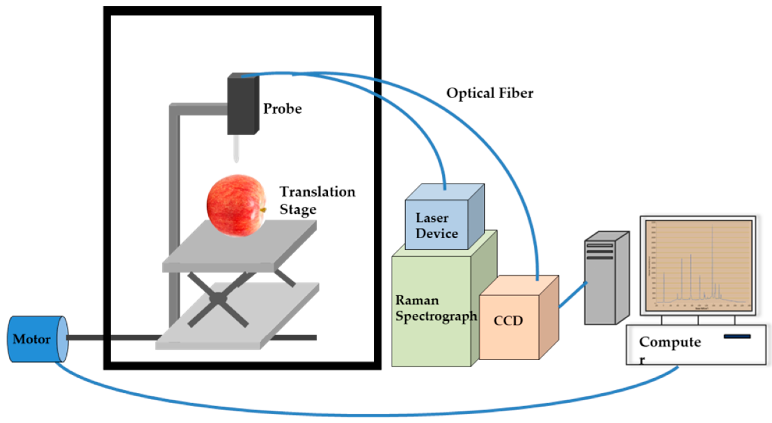
3.1. Optimization of Exposure Time and Laser Power
Appropriate parameter values were essential in the detection. The main parameters included exposure time and laser power. For samples with high pesticide concentration, the signal of characteristic peaks was easy to obtain. However, when the concentration of samples was low, the signal of the characteristic peaks would be weak or disappear if the exposure time was short or the laser power was small. While too long exposure time and too great laser power would lead to signal saturation or samples being burned by laser. Longer exposure time would also lead to time wasting for sample detection and may cause damage to charge-coupled device (CCD) camera. Thus it was necessary to optimize exposure time and laser power before the detection. Different exposure time and power were applied for detecting samples with same concentration. It can be seen that when the laser power was certain, the longer the exposure time was, the stronger the characteristic peak signal was. And when the exposure time or the laser power was short, the signal of the characteristic peaks could hardly be observed. Finally when the exposure time was 3s and the laser power was 450 mW, the signal of characteristic peak was the strongest. The maximum power of the laser was 450 mW. Laser of 450 mW would not damage the apple samples. Hence the laser was set at 450 mW. If the exposure time exceeds 3 s, the signal may saturate and the CCD camera may be damaged.
3.2. Data Preprocessing and Analysis
When Raman spectroscopy was used for sample analyze, signal noise and fluorescence background were important factors which affect the accuracy of the analysis severely. The noise of the instrument, external environment, etc. leads to signal noise. In this study, the Savitzky-Golay (S-G) 5-point smoothing method [
19] was used to remove the spectral noise. This method was proposed by Savitzky and Golay and was widely used in data stream smoothing and noise reduction. And the method was a filtering method based on local polynomial least squares fitting in the time domain. The biggest advantage of the method was that it could ensure the shape and width of the signal while filtering out the noise.
Fluorescence background interference was the most important factor in Raman signal analysis especially for organic or biological samples, which made signal of the target analyte submerged. And accurate and effective removing fluorescence background was very important in Raman analysis. The principle of adaptive iterative reweighted penalty least squares (airPLS) was to control the fidelity and roughness of the fitting curve by weighting coefficients so as to obtain an ideal fitting curve in this study [
20,
21]. This method was time-saving and flexible. The weight of the overall variance between the baseline of the fit and the original signal was changed through iteration. The overall variance weight was acquired from the difference between the baseline and the original signal. The first derivative and second derivative methods could eliminate the interference from the baseline and other backgrounds effectively and improve the resolution and sensitivity. But the method may lead to an increase in the signal-noise ratio. The standard normal variable transformation could eliminate the Raman spectrum noise. It could not remove the fluorescence background interference due to the power change of the laser light source and the attenuation of the light intensity. Baseline calibration deducted the fluorescence background effectively and preserved the original spectral information and eliminated the effects of the instruments. Two baseline calibration methods, the polynomial fitting method of 8 times and the signal minimum maxima, were used in the study. Adaptive scaling was a common calibration method.
3.3. Pesticide Mixture Signal Analysis
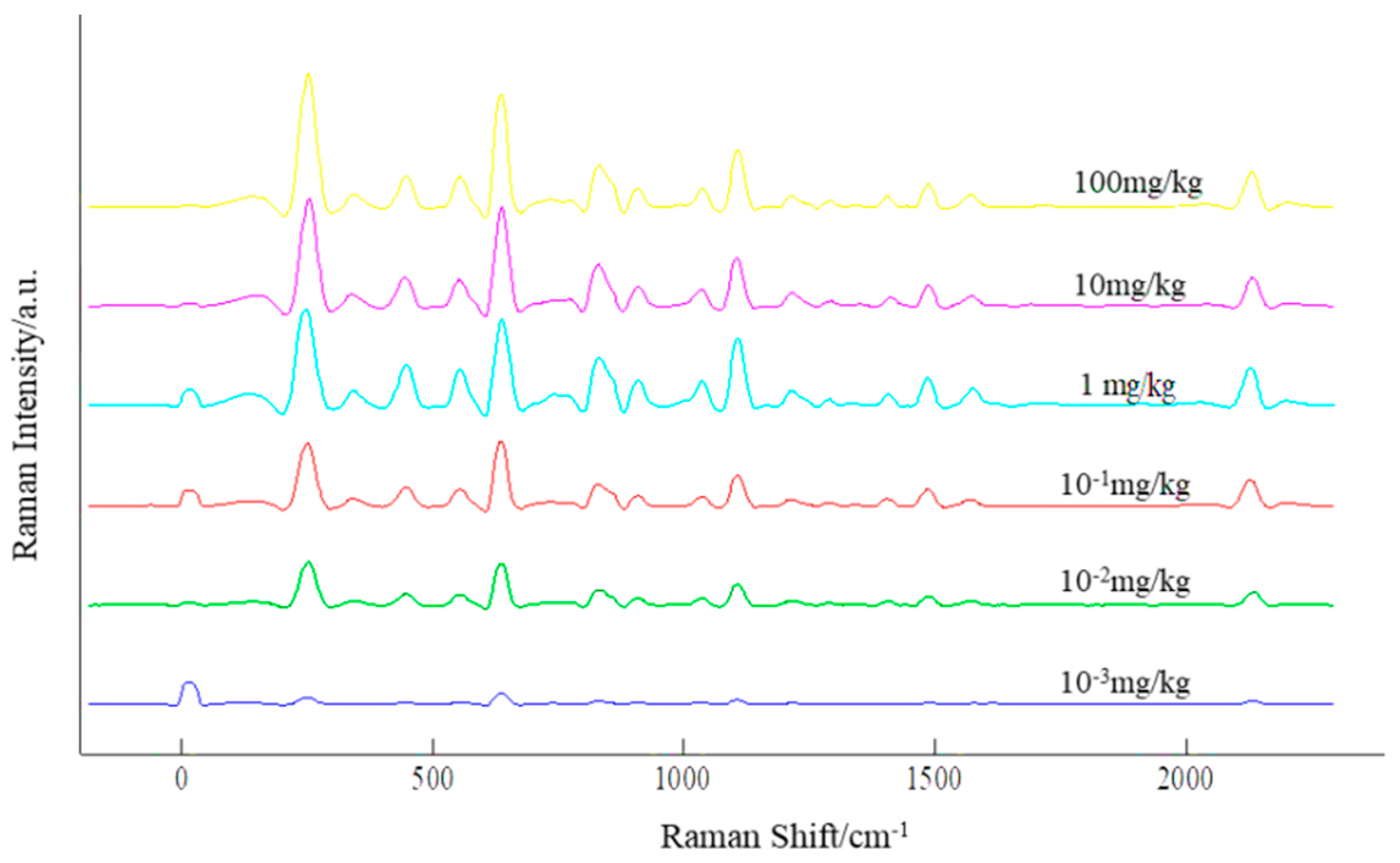
Surface-Enhanced Raman Scattering (SERS) signal acquisition was applied to standard solution of acetamiprid and deltamethrin pesticide and mixture of the two pesticides. There were literatures reported that main characteristic peaks of acetamiprid pesticide were located at 634, 1114 and 2164 cm
−1, and the characteristic peaks of deltamethrin were located at 574, 735 and 1380 cm
−1. Spectrum of characteristic peaks of pesticide mixture change with gradient concentration was shown in
Figure 2. In the spectrogram, the characteristic peaks of the two pesticides were obvious and the intensity of the characteristic peaks changed with the concentration of pesticides consistently. Thus it was certain that peaks at 634, 1114, 2164 cm
−1 and 574, 735, 1380 cm
−1 were characteristic peaks of acetamiprid and deltamethrin pesticide. Overlapping peak didn’t exist between acetamiprid and deltamethrin.
In Raman spectral detection, the characteristic peak intensity reflects the concentration of samples. Thus quantitative analysis could be made from Raman spectral signal. With the decrease of pesticide content, the intensity values of deltamethrin and acetamiprid characteristic peaks reduce linearly. As shown in
Figure 2.
The location of the Raman vibration peak was only related to the vibration frequency of the chemical bond. Raman spectral peaks in different locations represented different chemical bonds [
22]. According to common Raman spectral characteristic peak attribution map and comparison with other results analyze, it was possible to acquire the belonging of some characteristic peaks. Characteristic peaks of acetamiprid at 634, 1114 and 2167 cm
−1 belonged to C-Cl retraction, ring vibration, and ring “breathing” respectively. Characteristic peaks of deltamethrin at 574, 735, 1380 cm
−1 were caused by C-Br retractable, symmetrical CBr
2 flexing and ring scaling. The analysis results were consistent with the study by Dong [
23]. And apple samples would cause no obvious Raman spectral peaks [
24].
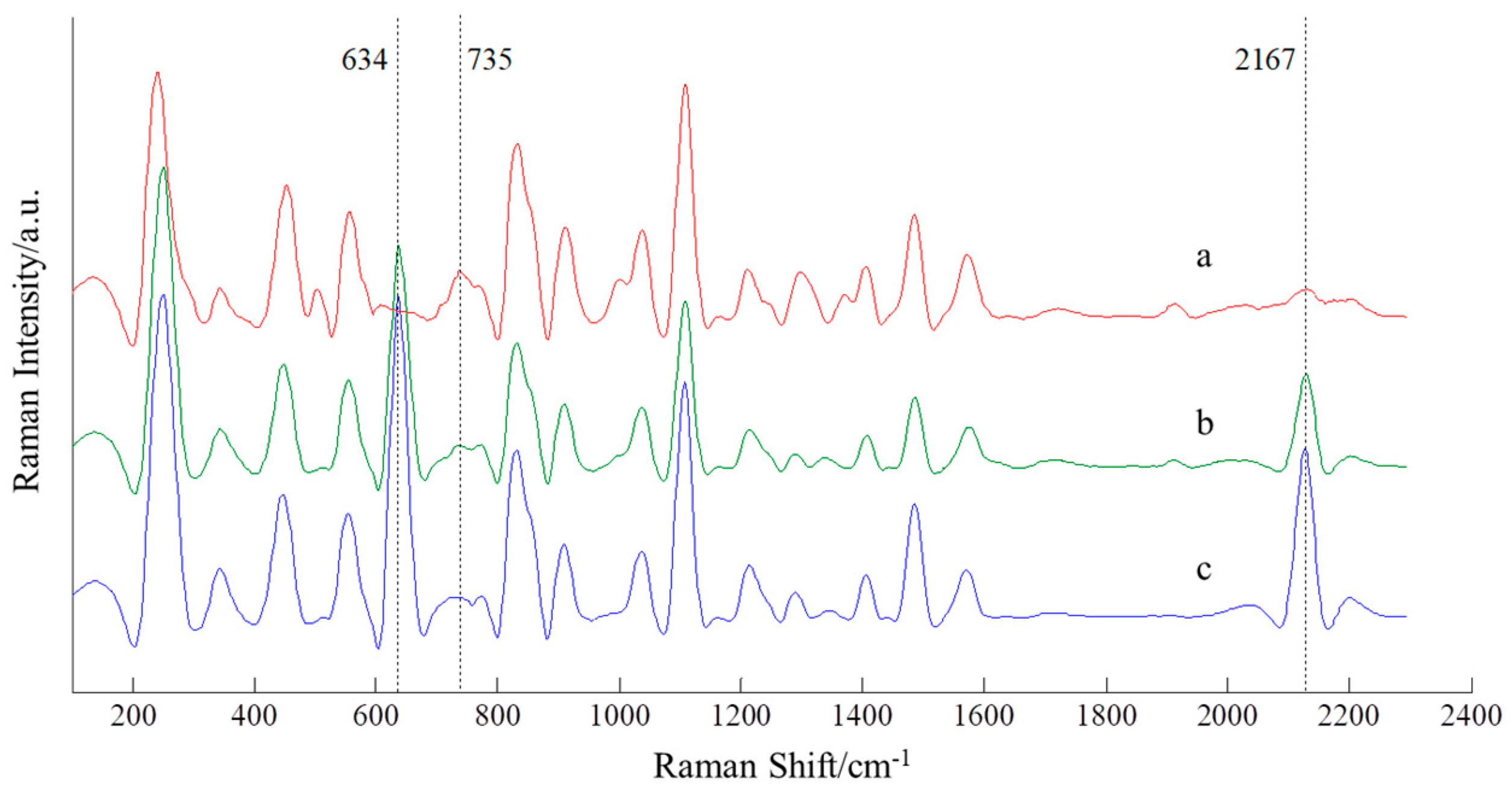
As deltamethrin and acetamiprid were always be used in the same agricultural season, it was necessary to detect the mixture of the two pesticides. It could be seen clearly from
Figure 3 that intensity of characteristic peaks of deltamethrin and acetamiprid pesticide mixture at 634, 1114 and 2167 cm
−1 was lower than the ones of single deltamethrin or acetamiprid pesticide solution, which affected the accuracy of detection result severely. It was clear that the intensity of characteristic peaks decreased when the other pesticide was added.
Table 1 showed the detection results comparison of gradient concentration mixed pesticides concentration and real pesticides concentration. Through analyzing original spectra of the two pesticides, it could be found that decrement of the peak intensity was in a certain extent. And the extent depended on the concentration of the two pesticides, exposure time of laser and integration time of CCD camera, mainly the concentration of pesticides. Therefore it was necessary to find out the link between the decrement extent of characteristic peaks and concentration of pesticides, and then to get the actual detection result.
By comparing a number of Raman spectra, it was clear to find that both characteristic peaks intensity value of single pesticide and pesticide mixture were steady in a range, which meant the multiple difference between single pesticide and pesticides mixture was certain. It was possible to find the ratio between characteristic peaks intensity value of single pesticide and the ones of pesticide mixture. Therefore the real peak intensity of one pesticide could be acquired through peak intensity of pesticides mixture and the ratios. The method of ratio would be realiable in Raman spectral detection of deltamethrin and acetamiprid mixture.
60 Fuji apples were used for detecting Raman spectral signals. 600 sample signals of deltamethrin, acetamiprid and the mixture of them were acquired. The Raman spectral information of deltamethrin, acetamiprid and the mixture of them with same pesticide concentration were detected from same apple sample to reduce the effect of sample background. Through analyzing massive full-spectrum Raman signal of deltamethrin and acetamiprid it was found that signal of characteristic peaks at 574, 1380 and 2167 cm−1 was not strong enough for quantitative analysis. Thus characteristic peaks at 634, 735 and 1114 cm−1 were used for data analysis of pesticide mixture.
3.4. Establishment of Regression Models
The mixture pesticides be detected included the deltamethrin and acetamiprid mixtures with same content and the ones with different concentration. As most pesticide mixture applied in farmland was in low content, detailed analyze of correction coefficient change rule was focused in low concentration. Deltamethrin, acetamiprid with concentration of 100, 10, 1, 10−1, 10−2 and 10−3 mg·kg−1 were mixed as mixture in pairs. And there were 36 mixed mode. At least 15 sample points would be detected to get the average as representative concentration in each mixed mode to make sure the representative.
The characteristic peak intensity of the pesticide detected directly cannot be directly used to predict the concentration of the mixed pesticide. By analyzing the reduction ratio of mixed pesticides characteristic peak intensity compared with the intensity of single pesticides, a model of mixed pesticides peak intensity correction coefficient was established. Firstly, the concentration of the mixed pesticide was estimated by a single pesticide quantitative analysis model to get the estimated pesticide concentration. And then the estimated pesticide concentration was applied in correction coefficient model to acquire the correction coefficient. The characteristic peak intensity of the pesticide was multiply by the correction coefficient to get the corrected peak intensity. Finally the corrected pesticide concentration was obtained by applying corrected peak intensity to quantitative analysis model of the pesticide.
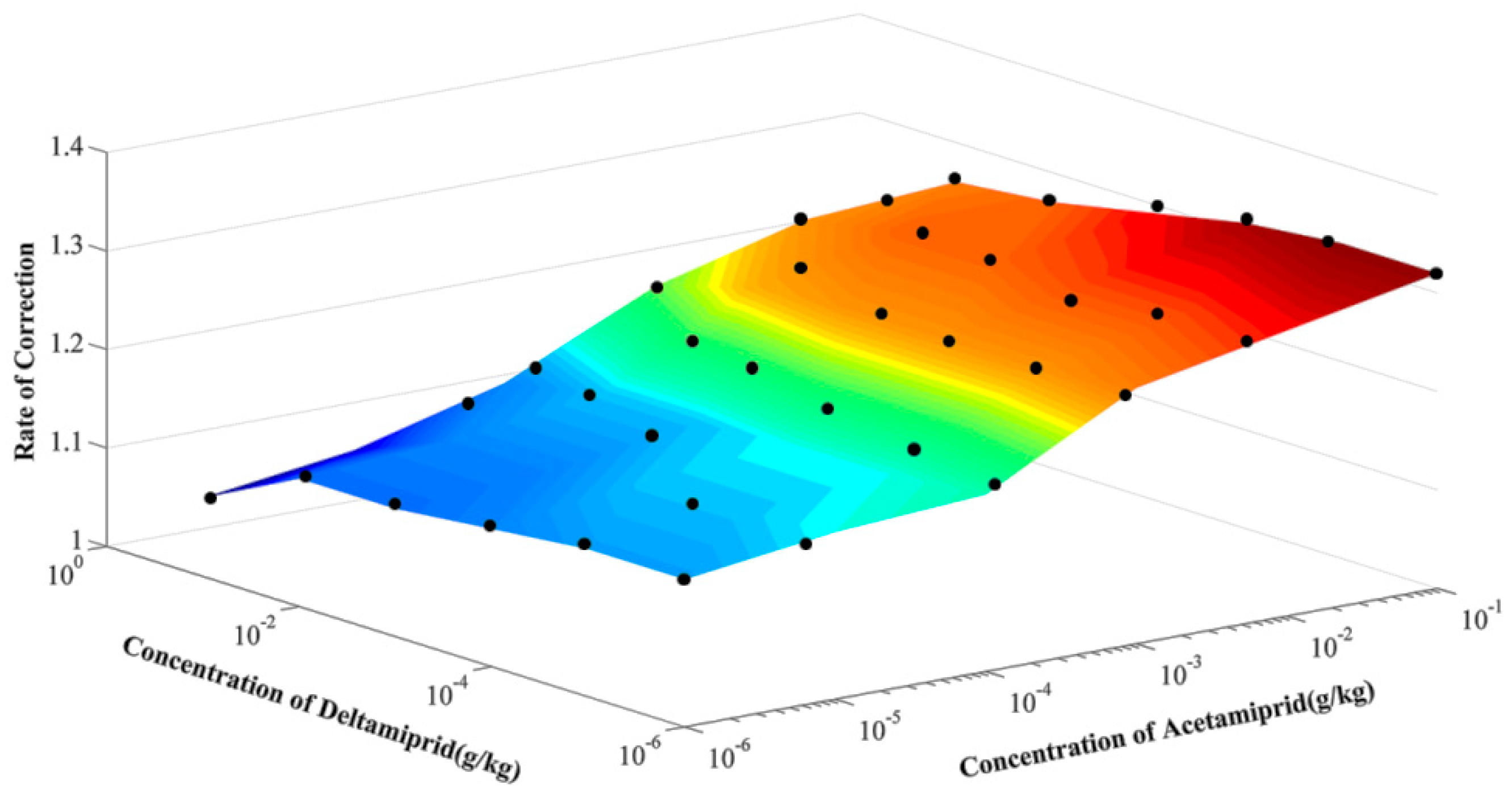
It was clear that correction coefficient change rule was the key to get accurate pesticide concentration. The correction coefficient was obtained by dividing the characteristic peak intensity value of a single pesticide by the characteristic peak intensity value of the pesticide mixture with same concentration. As quadratic function relations existed between pesticide concentration and the correction coefficients, two quadratic equations were needed to describe the change rule between content of pesticide mixture and the correction coefficients. And the change rule of one characteristic peak intensity was described by a binary quadratic polynomial.
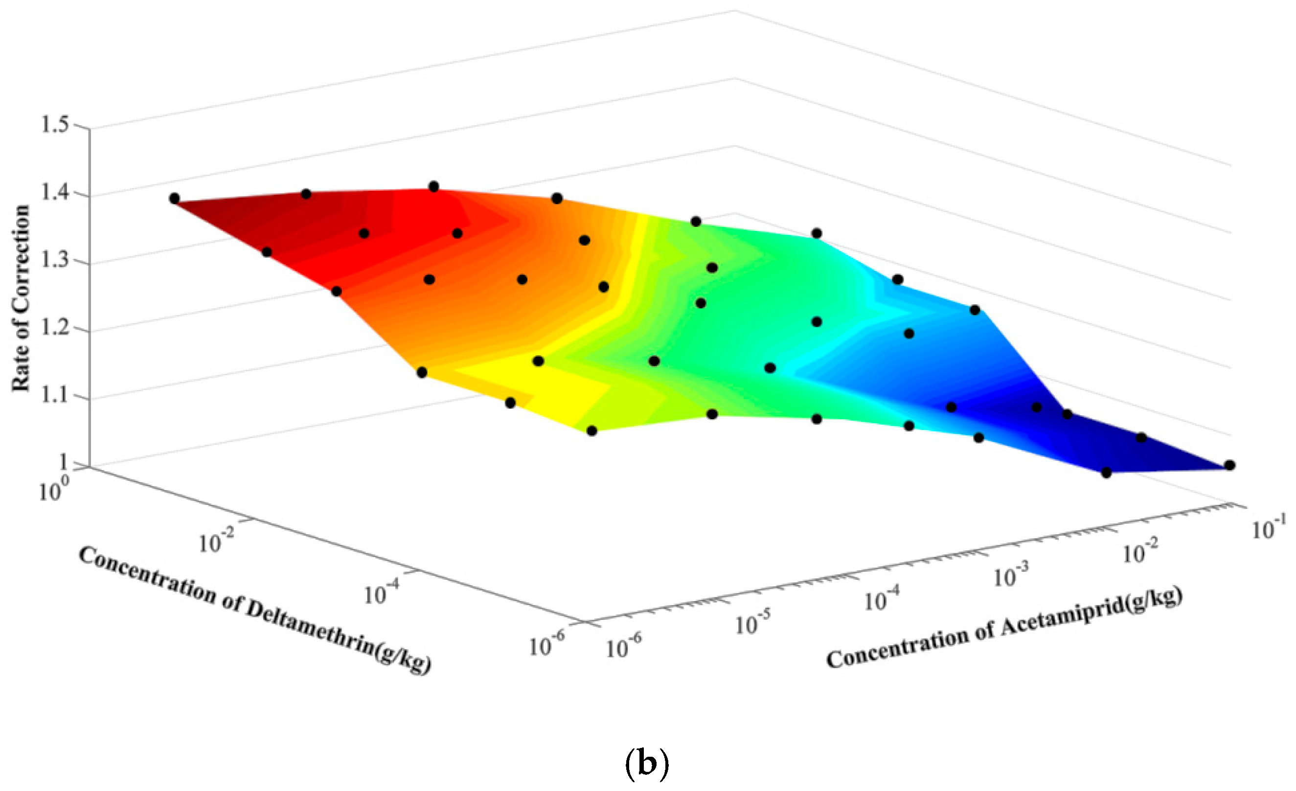
As shown in
Figure 4, the fitting effect of mixed pesticides concentrations and the correction coefficients was a smooth and slanted surface. For the characteristic peaks of acetamiprid at 634 cm
−1 and 1114 cm
−1, the correction coefficient reduced with not only the increments of acetamiprid concentration, but also the reduction of deltamethrin concentration. And when the concentration of one pesticide was low, its correction coefficient would be high, which indicated that components with low concentration in mixed pesticides were more likely to be affected by pesticides high concentration. For the change rule fitting model of peak in 634 cm
−1, the sum squared residual (SSE) was 0.0678. Root Mean Square Error (RMSE) and coefficient of correlation were 0.0475 and 0.9328 respectively. And for the change rule fitting model of peak in 1114 cm
−1, the SSE was 0.0328. RMSE and coefficient of correlation were 0.0330 and 0.8883 respectively.
A polynomial regression equation (Equation (1)) was acquired from the change rule fitting surface of characteristic peaks at 634cm
−1. In Equation (1), the concentrations of acetamiprid and deltamethrin were all from 100 mg·kg
−1 to 10
−3 mg·kg
−1.
where Z is the correction coefficient, A is the estimated concentration value of acetamiprid, D is the concentration value of deltamethrin.
The polynomial regression equation (Equation (2)) of characteristic peaks at 1114 cm
−1 was also obtained and shown below. In Equation (2), the concentrations of acetamiprid and deltamethrin were all from 100 mg·kg
−1 to 10
−3 mg·kg
−1.
where Z is the correction coefficient, A is the estimated concentration value of acetamiprid, D is the concentration value of deltamethrin.
The fitting surface of characteristic peak at 735 cm
−1 was shown in
Figure 5. And for the characteristic peaks of deltamethrin at 735 cm
−1, the correction coefficient increased with the increase of acetamiprid concentration and the decrease of deltamethrin concentration. With the increase of acetamiprid content and decrease of deltamethrin content, the correction coefficient could be up to 1.32. The sum squared residual (SSE) of the fitting model was 0.0438. Root Mean Square Error (RMSE) and coefficient of correlation were 0.0382 and 0.9266 respectively.
The polynomial regression Equation (Equation (3)) of characteristic peaks at 735 cm
−1 was acquired and shown below. In Equation (3), the concentrations of acetamiprid and deltamethrin were all from 100 mg·kg
−1 to 10
−3 mg·kg
−1.
where Z is the correction coefficient, A is the concentration value of acetamiprid, D is the concentration value of deltamethrin.
3.5. Validation of the Correction Models
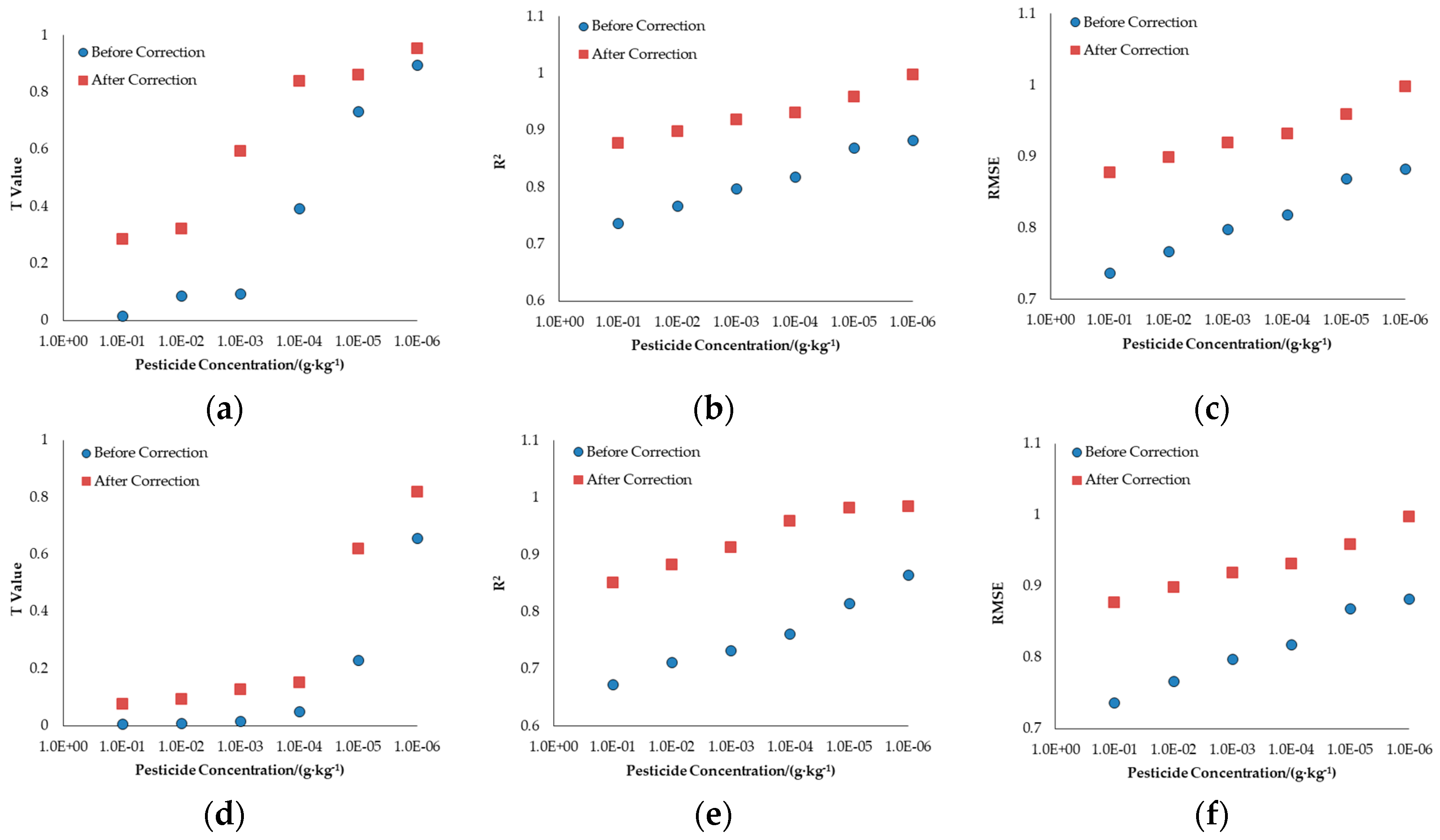
An experiment had been done to verify the reliability of the regression model. In the verification test of regression model, 200 deltamethrin and acetamiprid residue signals from 20 Fuji apples was set as validation set. The intensity of the characteristic peaks at 634, 735 and 1114 cm−1 was extracted from the Raman spectrum with pretreatment. Then the intensity values would be applied to the pesticide residue quantitative model to get the estimated pesticide concentration. Correction coefficient would be acquired after substituting peak intensity into the regression model. And corrected peak intensity would be obtained through multiplying the peak intensity values and correction coefficient. After substituting corrected peak intensity into pesticide residue quantitative model, corrected pesticide concentration would be got. Through comparing the pesticide concentration and corrected pesticide concentration, a series of parameters would be obtained to judge the regression model.
After above steps, Raman signals of validation were processed. The modeling effect was evaluated by T value, correlation coefficient (R
2) and Root Mean Squared Error (RMSE). The results were shown in
Figure 6. In
Figure 6, “●” and “■” stood for the pesticide data before and after correction respectively.
From the figure it could be seen that with the reduction of pesticide concentration, the parameters improved. It could be surmised that when the pesticide content increased, a plurality of pesticides molecules competed for the active sites provided by the silver sol. High concentration of pesticides resulted in a severe reduction in the number of active sites. And the other mixture molecules had fewer active sites and their characteristic peak signals were weaker correspondingly. When the pesticide concentration was relatively low, the number of silver sol active sites occupied by pesticide molecules was small. No obvious competitive relationship existed between pesticides. Therefore, one pesticide characteristic peak signal was not interfered by other pesticides. And all the parameters were improved obviously.
It could be seen from
Figure 6 that with the concentration of one pesticide decreasing, the correction coefficient of the other pesticide also decreased significantly. It could be deduced that the mutual influence of the functional groups of the two pesticide molecules which weakened each other caused this phenomenon. Concentration of pesticides functional groups reflected the characteristic peaks intensity, in turn reflecting the pesticides concentration. With the increase of one pesticide concentration, the influence of the other pesticide reduced gradually. This phenomenon may exist in other pesticide mixture and correction method would be useful in detecting them accurately.


