Abstract
Characterizing nonhomogeneous elastic property distribution of solids is of great significance in various engineering fields. In this paper, we observe that the solution to the inverse problem utilizing the standard optimization-based inverse approach is sensitive to the sizes of inclusions. The standard optimization-based inverse approach minimizes a cost function, containing the absolute error between the measured and computed displacements in L2 norm. To address this issue, we propose a novel inverse scheme to characterize nonhomogeneous shear modulus distribution of solids. In this novel method, the cost function is modified, and is dependent on the size of the inclusions. A number of simulated experiments are performed, and demonstrate that the proposed approach is capable of improving the shear modulus contrast in inclusions and reducing the size sensitivity. Furthermore, a theoretical analysis is conducted to validate what we have observed in simulated experiments. This theoretical analysis reveals that what we have observed in the simulated experiments is not induced by the numerical issues Instead, the size sensitivity issue is induced by regularization. The findings of this work encourage us to propose new cost functions for the optimization-based inverse approach to improve the quality of the shear modulus reconstruction.
1. Introduction
The advancement of high-resolution imaging modalities like digital imaging correlation (DIC) makes it possible for us to measure full-field displacement fields with high accuracy [1,2,3]. The measured full-fields displacement fields can be utilized to identify the nonhomogeneous elastic distribution of solids. Mapping the nonhomogeneous elastic distribution usually requires solving an inverse problem in elasticity. There are many inverse approaches that have been developed to solve the inverse problem, including virtual fields methods [4,5,6], optimization-based approaches [7,8], etc. Among them, optimization-based inverse approaches have been commonly used, as they are rigorous and highly robust. In the optimization-based inverse approach, the inverse problem in elasticity is posed to be a constrained minimization problem, where a cost function accounting for the discrepancy between measured and computed displacements is usually defined in the L2 norm and minimized iteratively. Since noise in the measured data will affect the quality of the final reconstructed results, regularization is introduced to prevent over-fitting. The regularization term is usually added as an additional term in the cost function (see Equation (3)). By setting an optimal weight for the regularization term, the inverse problem is solved without fully minimizing the displacement discrepancy term.
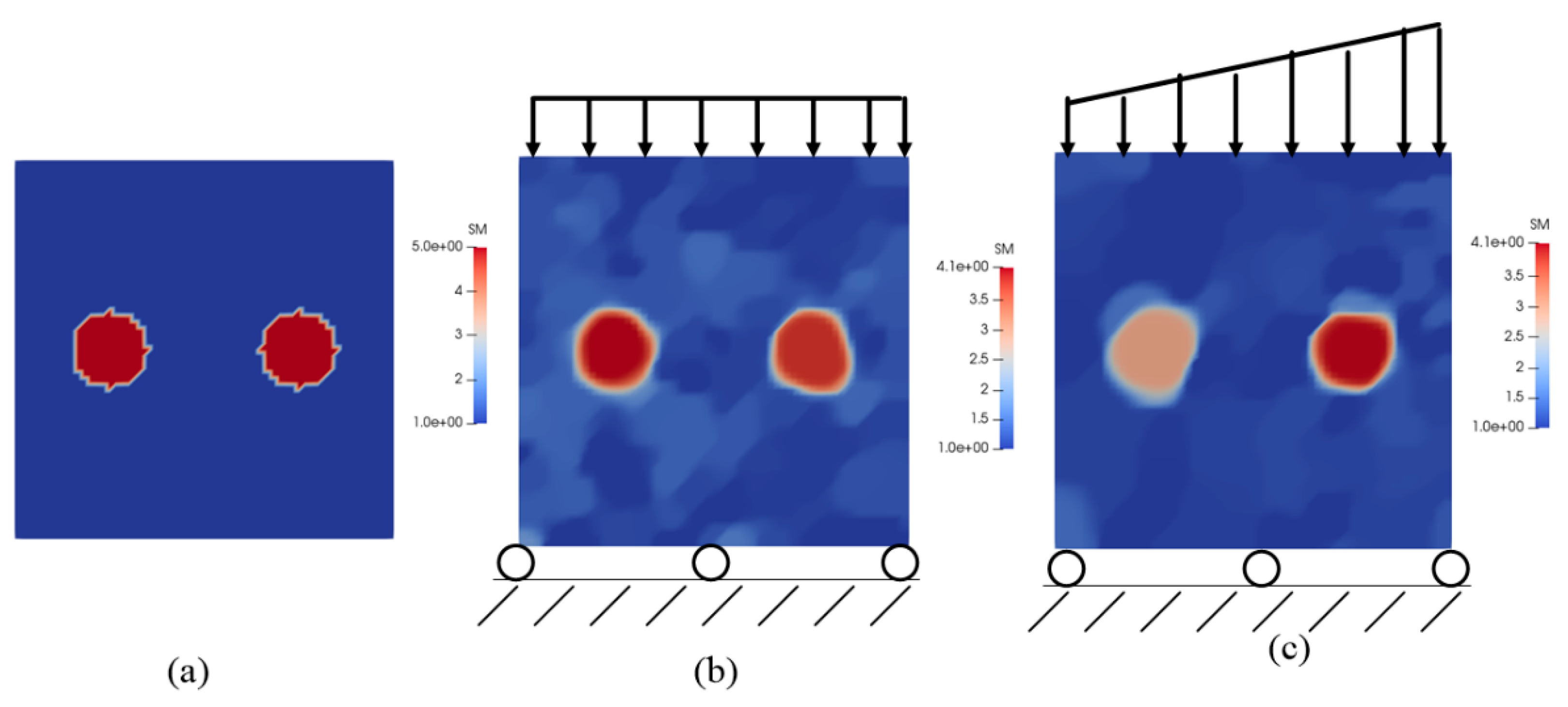
However, recent studies have revealed that the cost function that minimizes the absolute error in the displacement discrepancy term does not perform well in some practical cases. In [9], the authors found that the solution to the inverse problem utilizing this standard cost function is boundary-sensitive. That is, the reconstructed elastic property distribution of solids is sensitive to the prescribed boundary conditions (see Figure 1).
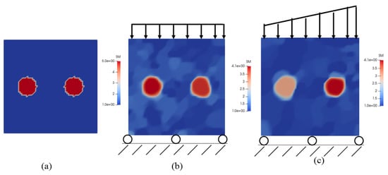
Figure 1.
(a) Target shear modulus distribution. (b) Reconstructed shear modulus distribution when the loading is uniform. (c) Reconstructed shear modulus distribution when the loading is non-uniform.
To address this issue, a modified cost function was proposed and significantly improved the reconstruction results—in particular, the stiffness contrast between different heterogeneous regions (reconstructed shear moduli in inclusions in Figure 1). The modified cost function was spatially weighted by the strain fields.
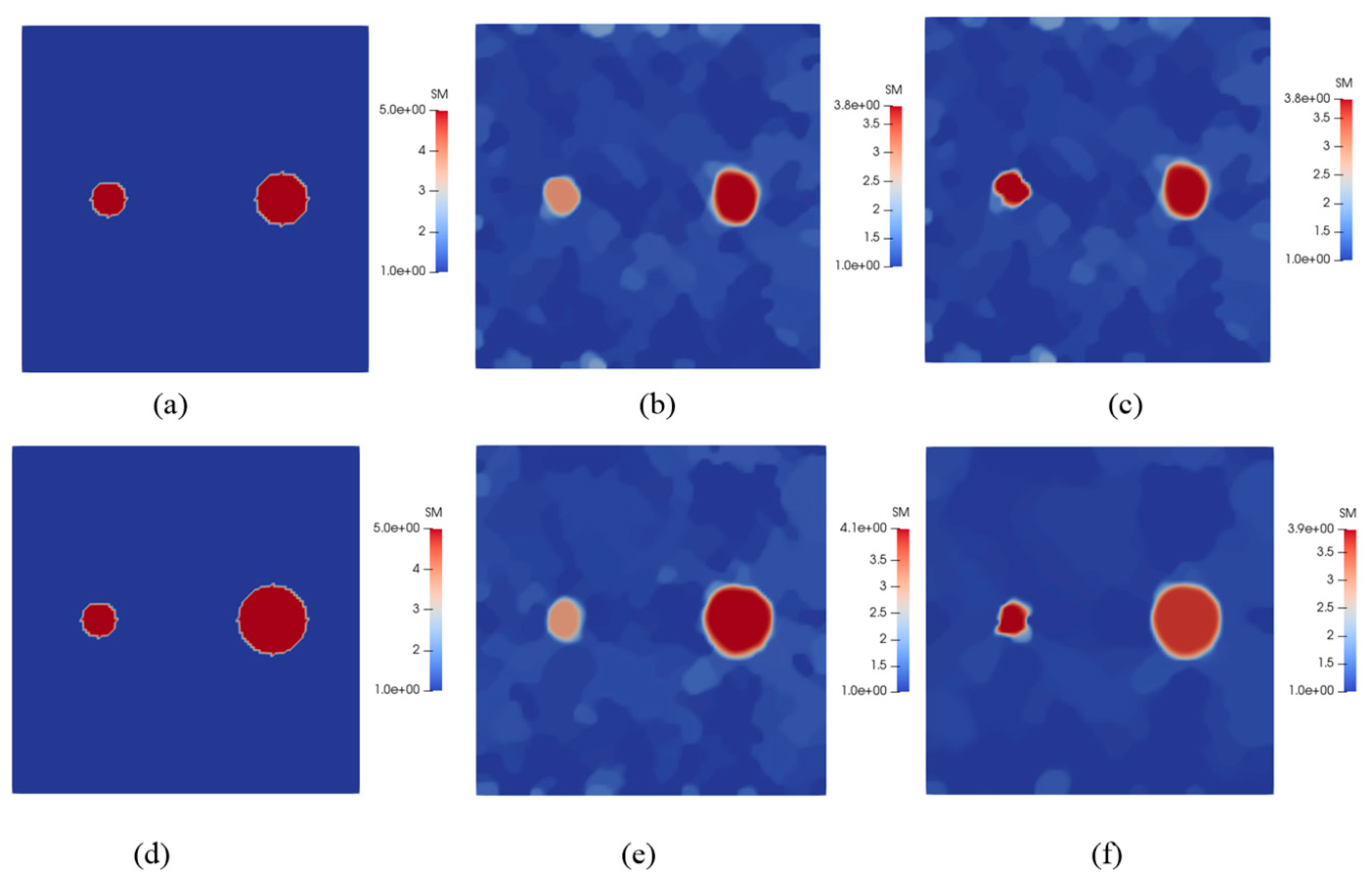
In this paper, we will investigate another limitation of the standard optimization-based inverse approach. That is, the solution to the inverse problem depends on the size of the inclusions (see Figure 2). To address this issue, a novel cost function that is size-dependent will be proposed. The solid studied in this paper is assumed to be incompressible linear elasticity. We will adopt a number of simulations and a simple theoretical analysis to show why the proposed approach performs better than the standard approach.
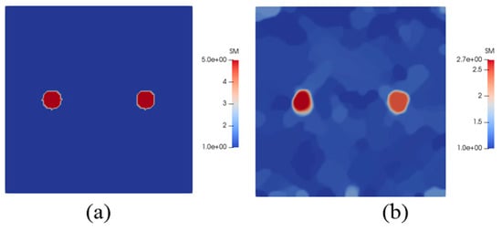
Figure 2.
(a) Target shear modulus distribution where two inclusions are of the same size. (b) Reconstructed shear modulus distribution with a regularization factor of 3.0 × 10⁻¹⁰.
The paper is organized as follows. We will first discuss the standard and proposed inverse algorithms in Methods section. We will then solve the inverse problem of elasticity by both methods with the simulated displacement fields acquired by finite element simulations, in the Results section. To understand the performance of the standard and proposed inverse approaches, we will employ a one-dimensional (1-D) model composed of two elastic bars and perform a simple theoretical analysis. Afterwards, we will thoroughly elaborate the reconstruction results in the Discussion section.
2. Methods
2.1. Forward Problem
The forward problem in linear elasticity is defined as follows:
where div is the divergence operator; and are the stress tensor and displacement vector, respectively; and are the displacement and traction values on the displacement and traction boundaries and , respectively; and constitutes the entire boundary of the domain . In addition, n is the outward normal vector. The incompressible linear elastic assumption is made in this paper, and the associated stress–strain relation in two-dimensional cases is written as follows:
where is the shear modulus; p is the hydrostatic pressure; and and I are the strain and identity tensors, respectively. To solve Equations (1) and (2), we adopt the finite element approach in this paper.
2.2. Inverse Problem
The inverse problem is solved by an optimization-based algorithm [7], where a cost function is minimized. Typically, a L2 norm correlation term, that is, the absolute error of the measured and computed displacement fields, is used to define the cost function:
where nodally-defined and are the measured and computed displacement fields, respectively. The computed displacement field is acquired by solving the forward problem using the finite element method at the current estimated shear modulus distribution of the domain of interest. The second term n Equation (3) is the total variation diminishing (TVD) regularization term to regularize the inverse problem. In addition, is the regularization factor determining the significance of regularization term and chosen by smoothness criteria [10], while is a small constant that resolves the singularity issue when computing the gradients of the cost function with respect to nodal shear moduli. The inverse problem is solved by a quasi-Newton approach referred to as the L-BFGS method [11,12]. The gradients of the cost function with respect to the nodal shear moduli are evaluated efficiently by the adjoint method [7].
In this paper, we propose a novel approach to address the issue that the solution to the inverse problem in elasticity is dependent on the size of the inclusions (see Figure 3b,e). The approach is divided into the following steps. First, we adopt the inverse approach with the standard cost function (Equation (3)) to detect the location of different heterogeneous regions. Second, we delimitate and compute the area of each inclusion from the reconstructed shear modulus distribution. Finally, we solve the inverse problem again by optimization-based inverse algorithms, with the following size-dependent cost function:
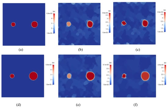
Figure 3.
In the first row, the target and reconstructed shear modulus distributions, where the target right inclusion is 1.5 times as large as the left one, are shown. In the second row, the target and reconstructed shear modulus distributions, where the target right inclusion is twice as large as the left one, are presented. (a) Target shear modulus distribution where the right inclusion is 1.5 times as large as the left one. (b) Reconstructed shear modulus distribution with the regularization factor of 2.0 × 10⁻¹⁰, utilizing the standard method. (c) Reconstructed shear modulus distribution with the regularization factor of 2.0 × 10⁻¹⁰, utilizing the proposed method. (d) Target shear modulus distribution where the right inclusion is twice as large as the left one. (e) Reconstructed shear modulus distribution with the regularization factor of 2.0 × 10⁻¹⁰ utilizing the standard method. (f) Reconstructed shear modulus distribution with the regularization factor of 4.0 × 10⁻¹⁰ utilizing the proposed method.
is a weight function depending on the normalized area of the i-th inclusion. That is, for the nodes within the i-th inclusion, is the area ratio between the i-th inclusion and the smallest inclusion (the areas of the i-th inclusion and the smallest inclusion are denoted by and , respectively). For the background of the domain of interest, . In the next section, we will employ the proposed approach to solve the inverse problem.
3. Results
3.1. Modulus Reconstruction Acquired by Simulated Data
We test the standard and newly proposed inverse algorithms by the simulated data. The displacement fields are acquired by solving forward problems with a known shear modulus distribution (see Figure 2a), assuming that the solid is in the state of the incompressible plane strain. The forward problem is solved by the stabilized finite element method [13]. In the target shear modulus distribution, there are two inclusions embedded in the soft background. The stiffness ratio between the two inclusions and the background is 5:1. The size ratio between the right and left inclusions varies from 1 to 2. We applied 1% uniform compression on the top edge and restricted the vertical motion of the bottom edge. To prevent rigid body motion, we fix the center point of the bottom edge. The problem domain is discretized uniformly by 14,400 bilinear elements (120 elements along the x and y directions, respectively). To mimic the experimental data, we add 3% noise into the simulated displacement data. In addition, we utilize the vertical displacement component as the measured data in solving the inverse problem, since the displacements perpendicular to the direction of the compressive loading are usually measured with low precision in practice [14].
When these two inclusions have the same size (see Figure 2b), we observe that these two inclusions could be detected clearly from the background utilizing the standard inverse scheme. However, the shear modulus values of these two inclusions are roughly half of the target. This is probably due to the fact that the sizes of the inclusions are too small compared to the overall dimension of the problem domain. Thus, the shear modulus reconstruction is highly sensitive to the noise. We also find that the recovered shear modulus of the left is larger than that of the right inclusion, due to the noise effect.
When we increase the radius of the right inclusion (see Figure 3), the reconstructed results utilizing the standard approach demonstrate that the left inclusion is remarkably underestimated (see Figure 3b,e). Moreover, the underestimation became more significant when the size ratio between the two inclusions increases. More specifically, the recovered shear modulus contrast between the right and left inclusions increases from 1.3 to 1.4. The reason for this will be explained in the next section. When we utilize the proposed inverse approach (see Figure 3c,f), it is observed that the stiffness values of the left inclusion improve significantly. That is, the recovered shear modulus contrasts between the right and left inclusions for Figure 3c,f are 0.99 and 0.95, respectively. However, we also observe that the shape of left inclusion is slightly distorted compared to the shear modulus reconstruction by the standard approach. This is because the weight of the nodes in the inclusion is inversely proportional to its area. Thus, the smaller inclusion gain more weight in the new cost function (Equation (4)), leading to the full minimization of displacements of the left inclusion in the new method.
3.2. Modulus Reconstruction by a One-Dimensional Coupled Model
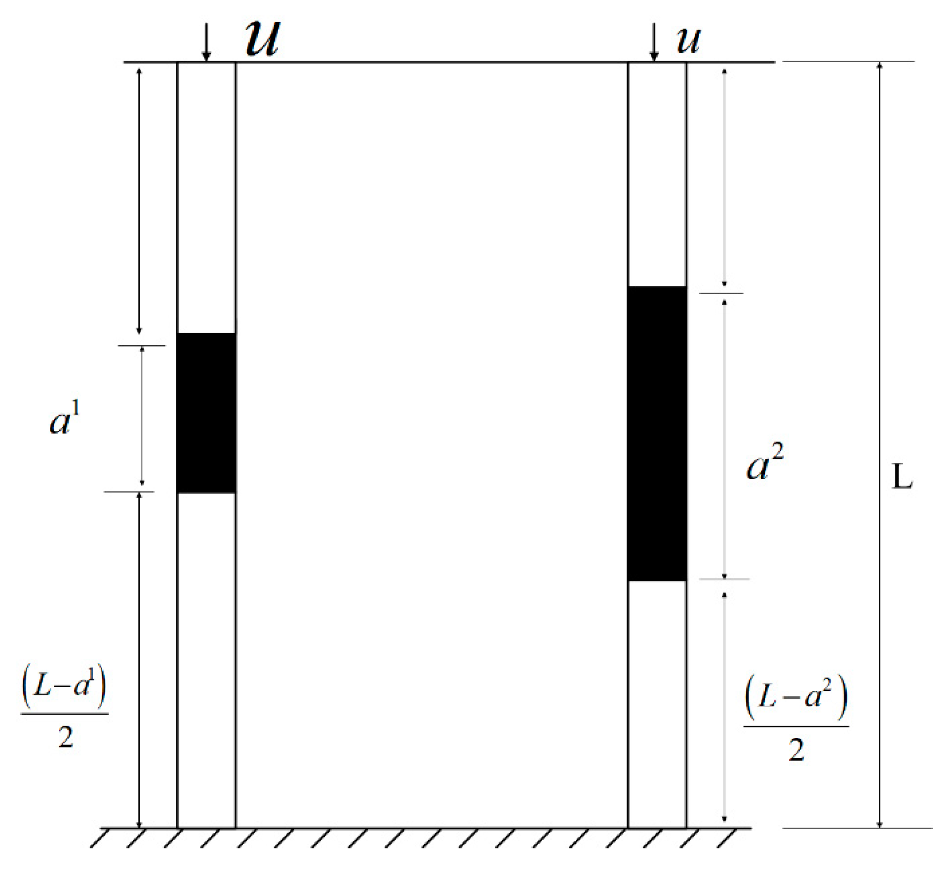
To represent enormous cases with varying sizes and shear moduli of these two inclusions, we employ an 1-D coupled model for analysis, shown in Figure 4. In Figure 4, the black regions in the two elastic bars represent two inclusions in the two-dimensional (2-D) cases presented in Section 3.1, and the rest denotes the background. The target shear modulus value of the background is fixed to be 1. The target shear modulus of the left and right inclusions is . In this case, the cost function in the standard approach can be simplified to
where i = 1 denotes the variables for the left and right bars, and denotes the recovered shear modulus value in the inclusion of the i-th bar. The recovered shear modulus value of the background is assumed to be reconstructed perfectly, thus being equal to 1.
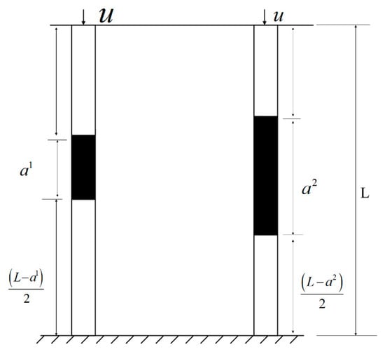
Figure 4.
A coupled one-dimensional (1-D) model: two linearly elastic and nonhomogeneous bars connected by two rigid plates.
To establish the relationship between and , we take the gradient of the cost function F with respect to and set it to zero. Accordingly, we reach the following relation:
where L and ai are the total length of each elastic bar and the size of the black region of the i-th bar. Since we have elaborated on a similar derivation in [15,16], we will not discuss herein.
For the proposed approach, the cost function is rewritten as
In this case, the relationship between the recovered shear moduli of these two inclusions is
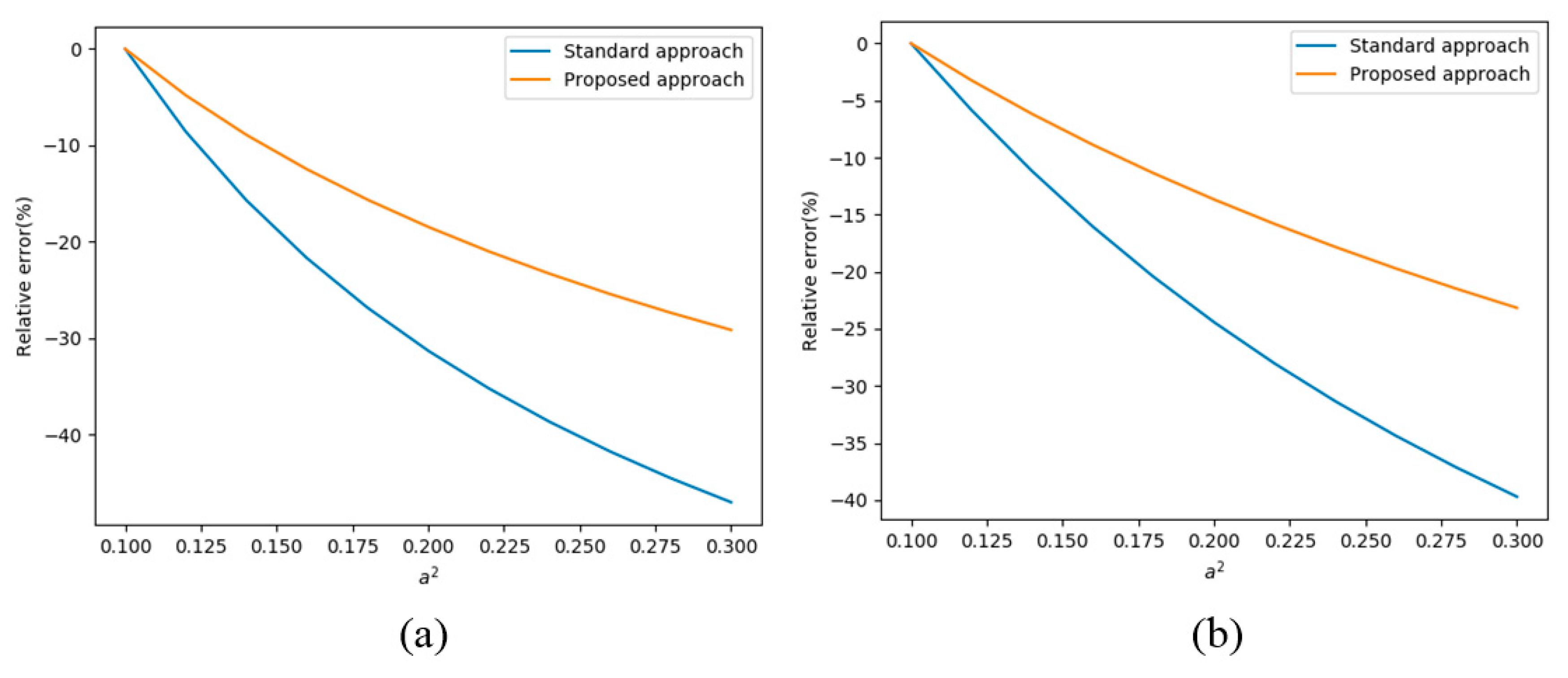
If the recovered shear modulus is determined, the recovered shear modulus of the inclusion of the left bar can be calculated via Equation (6) or Equation (8). Thus, we can quantitatively compare these two methods by the significance of the underestimation of shear modulus . More specifically, we assume that the recovered shear modulus of the right bar is underestimated by ε. To this end, , and should be , as the target shear moduli of these two inclusions are the same. We define a relative error as , and compute the relative error with varying sizes of the right inclusion , as shown in Figure 5. In Figure 5, the length of these two bars L, the size of the left inclusion , and the target shear modulus are fixed to be 1, 0.1, and 5, respectively.
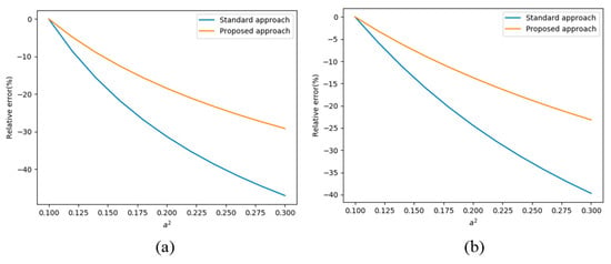
Figure 5.
(a)The variation of the relative error defined above with respect to the size of the right inclusion, , with underestimation . (b) The variation of the relative error defined above with respect to with .
Figure 5 demonstrates that when the sizes of these two inclusions are the same, then , indicating no error in the reconstruction. However, increasing the size of the right inclusion causes underestimation in the shear moduli of the left inclusion, as the relative error is negative in both methods. The underestimation becomes more serious with the increase of the size of the right inclusion. Importantly, employing the proposed approach is capable of significantly reducing the relative error. This result is consistent with what we have observed in the 2-D simulated experiments presented in Section 3.1.
4. Discussion
This paper presents a novel inverse method to characterize the shear modulus distribution of solids. This method modifies the standard cost function that minimizes the absolute error between the measured and computed displacements, and it is capable of improving the shear modulus contrast of inclusions with varying sizes. We have performed a number of 2-D numerical simulations to test the feasibility of this approach, and compared the performance of the standard and proposed approaches. The reconstruction results revealed that the proposed approach performs much better than the standard method, and improves the shear modulus contrast in the inclusions significantly. Additionally, a 1-D theoretical analysis was conducted to validate what we have observed in 2-D simulations.
The simulations presented in Section 3.1 revealed that the solution to the inverse problem utilizing the standard approach is size-dependent. More specifically, the smaller inclusion was underestimated, and the underestimation became more significant with the reduction of the size of the inclusion. To address this size-sensitivity issue, a modified cost function depending on the size of the inclusion was proposed in this paper. The new approach improved the shear modulus contrast in inclusions remarkably. In fact, the limitation of the standard L2 norm-based optimization inverse approaches was also discussed in [16]. The authors in [16] observed that the solution to the inverse problem by minimizing the standard L2 norm cost function is boundary-sensitive (see Figure 1). Therefore, minimizing L2 norm cost function might not be an optimal way to solve the inverse problem in practical engineering to characterize mechanical property distribution of solids.
We also employed an 1-D theoretical analysis to compare the new and standard approaches with a wide range of size ratios of the two inclusions (see Figure 5). The main merit of this 1-D analysis is that a large number of cases can be tested within seconds. This analysis showed that the new approach reduced the relative error in the shear modulus contrast in the inclusions with different sizes. We should note that we utilized the exact simulated displacement data to evaluate Equations (6) and (8) without introducing noise, since the underestimation of the shear modulus contrast in inclusions using the standard inverse approach is induced by the regularization. Though the new approach is capable of improving the shear modulus contrast in inclusions, the recovered shear modulus of the smaller inclusion is still underestimated, particularly in cases with a larger size ratio of the inclusions. In addition, we merely restricts our attention in the size sensitivity issue in this paper, but do not consider the boundary sensitivity issue. Thus, an improved and more general approach should be proposed in future work to completely resolve the issue. Besides, the displacement data can be obtained in high resolution by digital imaging correlation (DIC) [15,17,18,19]. In the future, we will test the proposed approach using experimental data from the DIC system.
5. Conclusions
This paper presents a novel inverse method to reconstruct nonhomogeneous shear modulus distribution of solids. The proposed inverse approach is capable of reducing the sensitivity of the solution of the inverse problem to the size of the inclusions. A number of numerical experiments have been conducted to test the feasibility of the novel approach. From these simulations, we observed that the novel approach significantly improved the shear modulus contrast in the inclusions. In addition, we have investigated a theoretical model and varied the size of the inclusions to validate what we have observed in simulations. This study will strengthen our understanding of the limitation of the standard, optimization-based inverse approach, which minimizes the absolute error between the measured and computed displacements in the L2 norm and triggers us to propose optimal inverse approaches to identify the nonhomogeneous mechanical property distribution of solids with high accuracy.
Author Contributions
Conceptualization, Y.M.; methodology, Y.M.; software, Y.M.; validation, X.Z., Y.S., and Y.M.; formal analysis, X.Z.; investigation, X.Z., Y.S., and Y.M.; resources, Y.M.; data curation, X.Z. and Y.S.; writing—original draft preparation, X.Z., Y.S., and Y.M.; writing—review and editing, X.Z., Y.S., and Y.M.; visualization, X.Z. and Y.S.; supervision, Y.M.; project administration, Y.M.; funding acquisition, X.Z.
Funding
This research was funded by the Natural Foundation of Shandong Province, grant number ZR2018BEE012 (Xinbo Zhao). Yue Mei also acknowledges the support from the Fundamental Research Funds for the Central Universities (Grant No. DUT19RC(3)017).
Conflicts of Interest
The authors declare no conflict of interest.
References
- Rossi, M.; Cortese, L.; Genovese, K.; Lattanzi, A.; Nalli, F.; Pierron, F. Evaluation of volume deformation from surface DIC measurement. Exp. Mech. 2018, 58, 1181–1194. [Google Scholar] [CrossRef]
- Dufour, J.-E.; Beaubier, B.; Hild, F.; Roux, S. CAD-based displacement measurements with stereo-DIC. Exp. Mech. 2015, 55, 1657–1668. [Google Scholar] [CrossRef]
- Passieux, J.-C.; Bugarin, F.; David, C.; Périé, J.-N.; Robert, L. Multiscale Displacement Field Measurement Using Digital Image Correlation: Application to the Identification of Elastic Properties. Exp. Mech. 2015, 55, 121–137. [Google Scholar] [CrossRef]
- Avril, S.; Huntley, J.; Pierron, F.; Steele, D. 3D heterogeneous stiffness reconstruction using MRI and the virtual fields method. Exp. Mech. 2008, 48, 479–494. [Google Scholar] [CrossRef]
- Pierron, F.; Grédiac, M. The Virtual Fields Method: Extracting Constitutive Mechanical Parameters from Full-Field Deformation Measurements; Springer Science & Business Media: New York, NY, USA, 2012. [Google Scholar]
- Nguyen, T.T.; Huntley, J.M.; Ashcroft, I.A.; Ruiz, P.D.; Pierron, F. A Fourier-series-based virtual fields method for the identification of 2-D stiffness distributions. Int. J. Numer. Methods Eng. 2014, 98, 917–936. [Google Scholar] [CrossRef]
- Oberai, A.A.; Gokhale, N.H.; Feijóo, G.R. Solution of inverse problems in elasticity imaging using the adjoint method. Inverse Probl. 2003, 19, 297. [Google Scholar] [CrossRef]
- Goenezen, S.; Barbone, P.; Oberai, A.A. Solution of the nonlinear elasticity imaging inverse problem: The incompressible case. Comput. Methods Appl. Mech. Eng. 2011, 200, 1406–1420. [Google Scholar] [CrossRef] [PubMed]
- Mei, Y.; Goenezen, S. Spatially weighted objective function to solve the inverse problem in elasticity for the elastic property distribution. In Computational Biomechanics for Medicine: New Approaches and New Applications; Doyle, B.J., Miller, K., Wittek, A., Nielson, P.M.F., Eds.; Springer: New York, NY, USA, 2015; Volume 6. [Google Scholar]
- Mei, Y.; Tajderi, M.; Goenezen, S. Regularizing biomechanical maps for partially known material properties. Int. J. Appl. Mech. 2017, 9, 1750020. [Google Scholar] [CrossRef]
- Zhu, C.; Byrd, R.H.; Lu, P.; Nocedal, J. L-BFGS-B: FORTRAN Subroutines for Large Scale Bound Constrained Optimization; Tech. Report, NAM-11; EECS Department, Northwestern University: Evanston, IL, USA, 1994. [Google Scholar]
- Zhu, C.; Byrd, R.H.; Lu, P.; Nocedal, J. L-BFGS-B: A Limited Memory FORTRAN Code for Solving Bound Constrained Optimization Problems; Tech. Report, NAM-11; EECS Department, Northwestern University: Evanston, IL, USA, 1994. [Google Scholar]
- Maniatty, A.M.; Liu, Y.; Klaas, O.; Shephard, M.S. Higher order stabilized finite element method for hyperelastic finite deformation. Comput. Methods Appl. Mech. Eng. 2002, 191, 1491–1503. [Google Scholar] [CrossRef]
- Pan, X.; Liu, K.; Bai, J.; Luo, J. A regularization-free elasticity reconstruction method for ultrasound elastography with freehand scan. Biomed. Eng. Online 2014, 13, 132. [Google Scholar] [CrossRef] [PubMed]
- Mei, Y.; Stover, B.; Kazerooni, N.A.; Srinivasa, A.; Hajhashemkhani, M.; Hematiyan, M.; Goenezen, S. A comparative study of two constitutive models within an inverse approach to determine the spatial stiffness distribution in soft materials. Int. J. Mech. Sci. 2018, 140, 446–454. [Google Scholar] [CrossRef]
- Mei, Y.; Kuznetsov, S.; Goenezen, S. Reduced boundary sensitivity and improved contrast of the regularized inverse problem solution in elasticity. J. Appl. Mech. 2016, 83, 031001. [Google Scholar] [CrossRef]
- Gerbig, D.; Bower, A.; Savic, V.; Hector, L.G. Coupling digital image correlation and finite element analysis to determine constitutive parameters in necking tensile specimens. Int. J. Solids Struct. 2016, 97, 496–509. [Google Scholar] [CrossRef]
- Mei, Y.; Wang, S.; Shen, X.; Rabke, S.; Goenezen, S. Mechanics Based Tomography: A Preliminary Feasibility Study. Sensors 2017, 17, 1075. [Google Scholar] [CrossRef] [PubMed]
- Avril, S.; Pierron, F.; Sutton, M.A.; Yan, J. Identification of elasto-visco-plastic parameters and characterization of Luders behavior using digital image correlation and the virtual fields method. Mech. Mater. 2008, 40, 729–742. [Google Scholar] [CrossRef]
© 2019 by the authors. Licensee MDPI, Basel, Switzerland. This article is an open access article distributed under the terms and conditions of the Creative Commons Attribution (CC BY) license (http://creativecommons.org/licenses/by/4.0/).

