Parametrizing the Conditionally Gaussian Prior Model for Source Localization with Reference to the P20/N20 Component of Median Nerve SEP/SEF

 ,
,  and
and
Abstract
:
1. Introduction
2. Methods
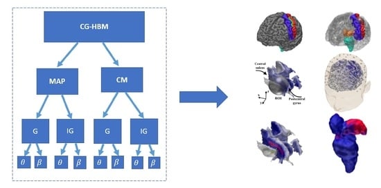
2.1. Conditionally Gaussian Hierarchical Bayesian Model
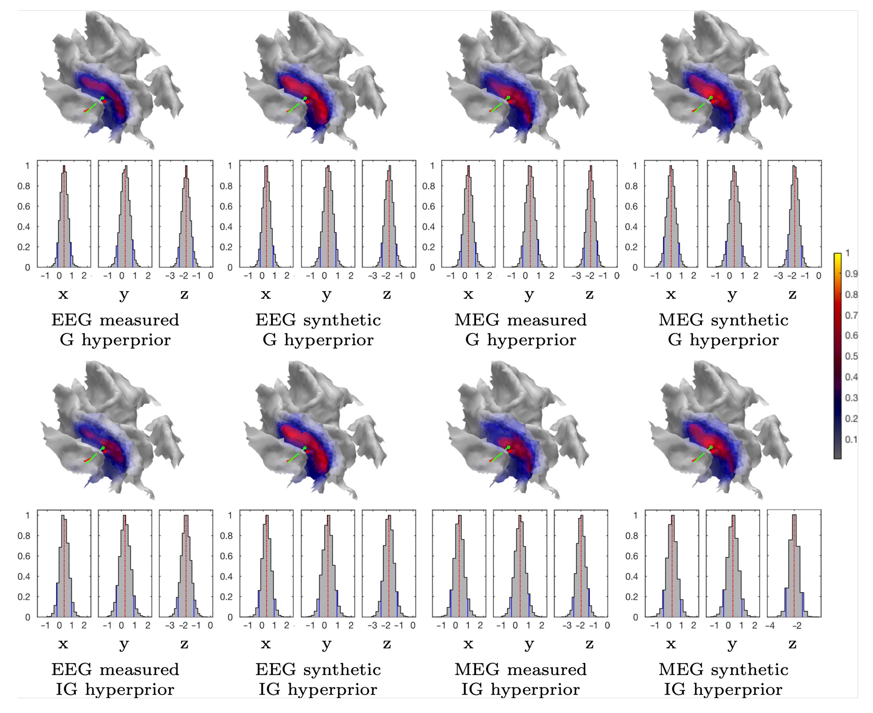
2.1.1. Posterior Exploration
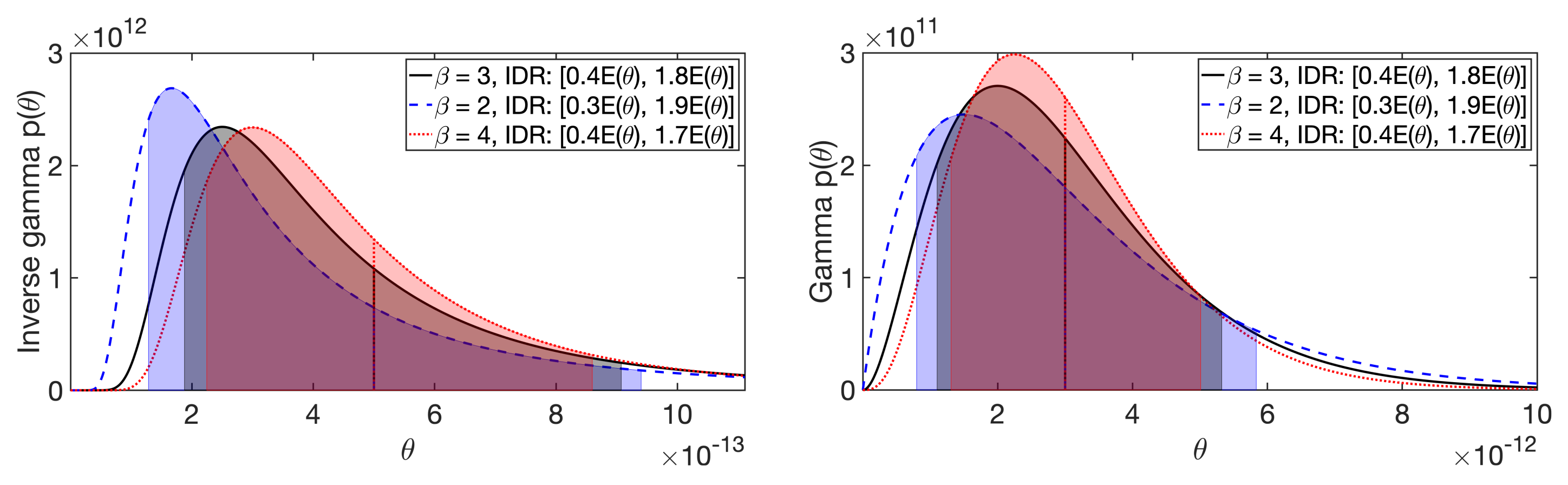
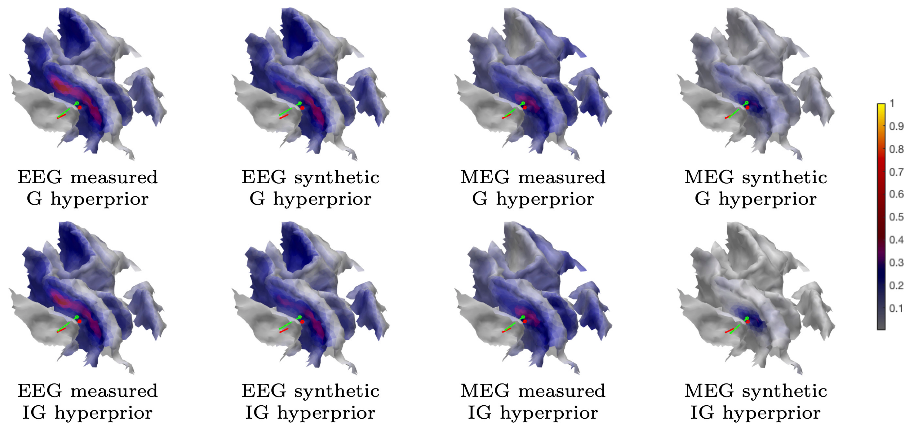
2.1.2. Gamma and Inverse Gamma Hyperprior
2.1.3. Total Scale
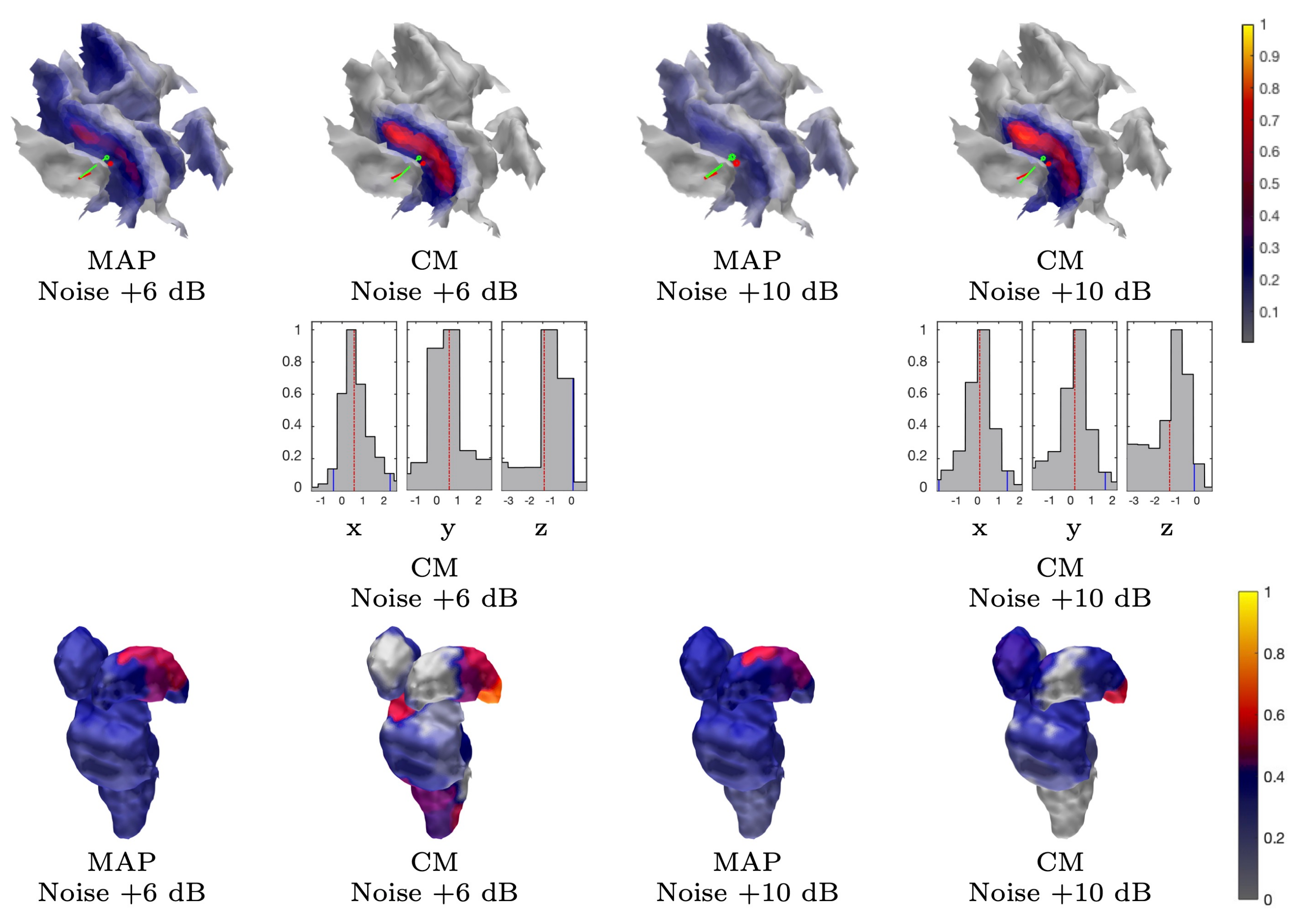
2.1.4. Latent Noise Effects
2.2. Numerical Model
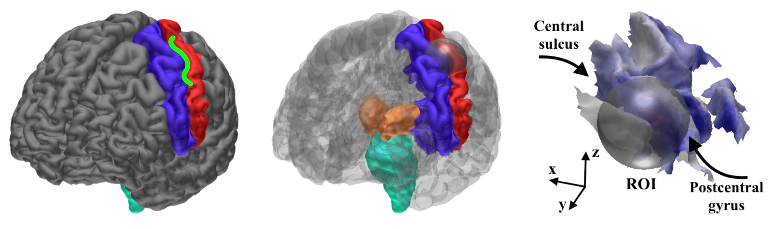
2.2.1. Head Segmentation
2.2.2. Source Space
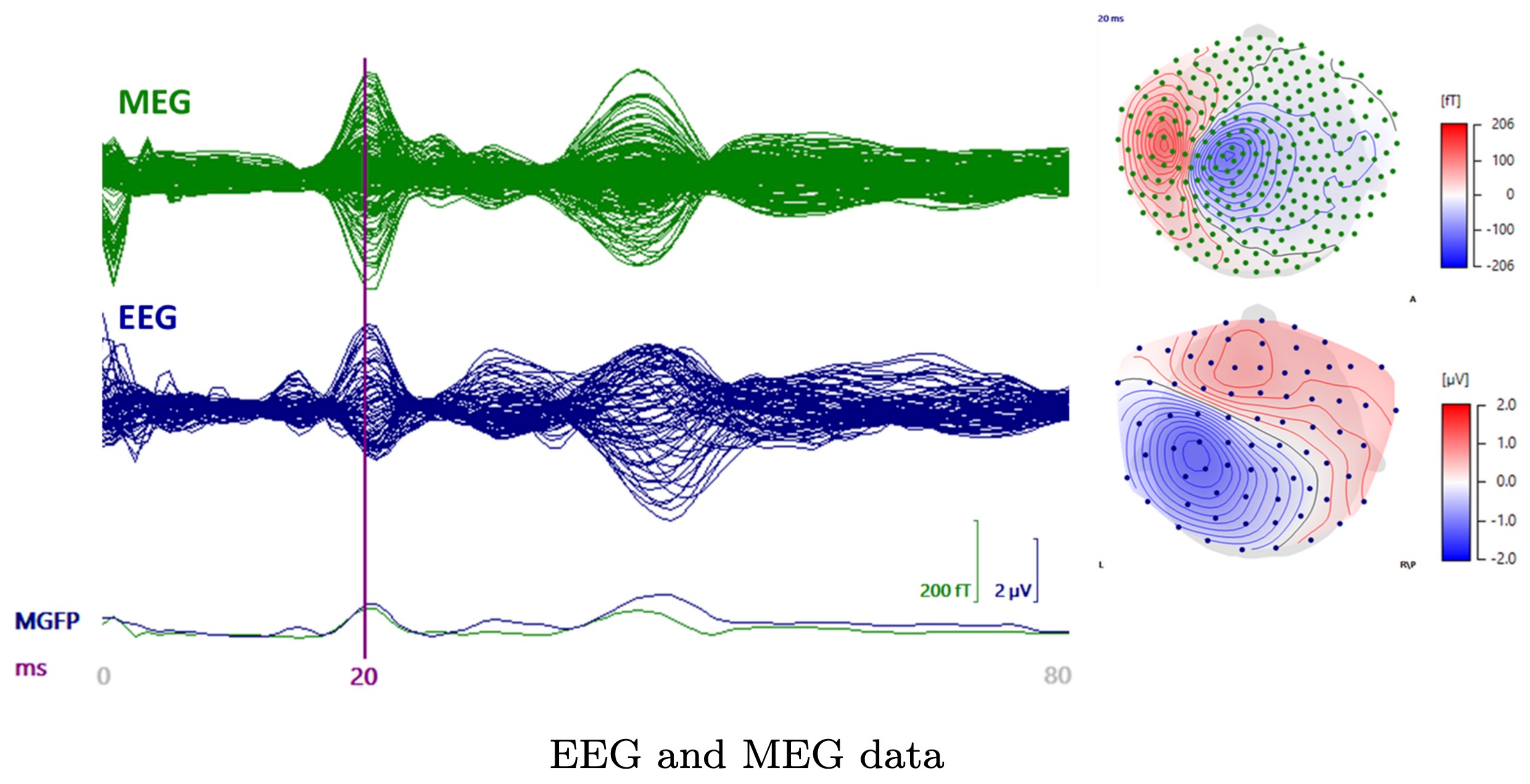
2.3. Measured Data
2.4. Synthetic Data
2.5. Source Localization Estimates
Implementation in Zeffiro Interface
3. Results
3.1. Subject (I)
3.1.1. Brodmann Area 3b
3.1.2. MAP Estimation
3.1.3. CM Estimation
3.1.4. Thalamic Component
3.2. Subject (II) and (III)
4. Discussion
Author Contributions
Funding
Conflicts of Interest
Appendix A. Shape Parameter Optimization
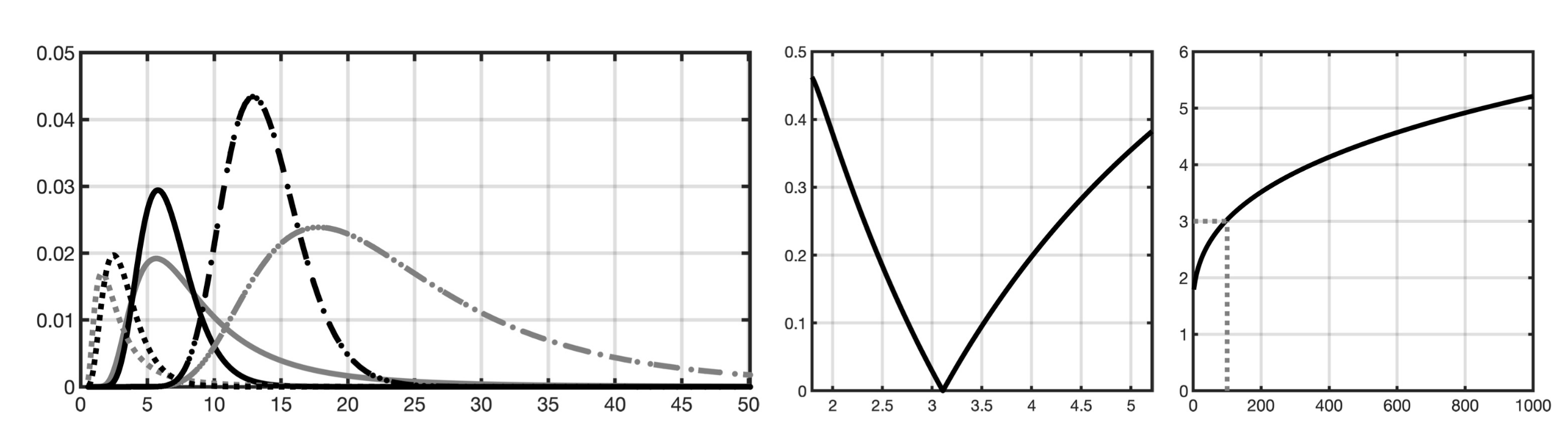
Appendix B. Effect of the Shape Parameter
References
- Hämäläinen, M.; Hari, R.; Ilmoniemi, R.J.; Knuutila, J.; Lounasmaa, O.V. Magnetoencephalography— Theory, instrumentation, and applications to invasive studies of the working human brain. Rev. Mod. Phys. 1993, 65, 413–498. [Google Scholar]
- Niedermeyer, E.; da Silva, F.L. Electroencephalography: Basic Principles, Clinical Applications, and Related Fields, 5th ed.; Lippincott Williams & Wilkins: Philadelphia, PA, USA, 2004. [Google Scholar]
- Brette, R.; Destexhe, A. Handbook of Neural Activity Measurement; Cambridge University Press: New York, NY, USA, 2012. [Google Scholar]
- Wipf, D.; Nagarajan, S. A unified Bayesian framework for MEG/EEG source imaging. NeuroImage 2009, 44, 947–966. [Google Scholar] [CrossRef] [PubMed] [Green Version]
- Friston, K.; Harrison, L.; Daunizeau, J.; kiebel, S.; Phillips, C.; Trujillo-Barreto, N.; Henson, R.; Flandin, G.; Mattout, J. Multiple sparse priors for the M/EEG inverse problem. NeuroImage 2008, 39, 1104–1120. [Google Scholar] [CrossRef] [PubMed]
- Sato, M.; Yoshioka, T.; Kajihara, S.; Toyama, K.; Goda, N.; Doya, K.; Kawato, M. Hierarchical bayesian estimation for MEG inverse problem. NeuroImage 2004, 23, 806–826. [Google Scholar] [CrossRef] [PubMed] [Green Version]
- Calvetti, D.; Hakula, H.; Pursiainen, S.; Somersalo, E. Conditionally Gaussian hypermodels for cerebral source localization. SIAM J. Imaging Sci. 2009, 2, 879–909. [Google Scholar] [CrossRef] [Green Version]
- Lucka, F.; Pursiainen, S.; Burger, M.; Wolters, C.H. Hierarchical bayesian inference for the EEG inverse problem using realistic FE head models: Depth localization and source separation for focal primary currents. NeuroImage 2012, 61, 1364–1382. [Google Scholar] [CrossRef] [PubMed]
- Ahlfors, S.P.; Han, J.; Belliveau, J.W.; Hämäläinen, M.S. Sensitivity of MEG and EEG to source orientation. Brain Topogr. 2010, 23, 227–232. [Google Scholar] [CrossRef] [Green Version]
- Hari, R.; Baillet, S.; Barnes, G.; Burgess, R.; Forss, N.; Gross, J.; Hämäläinen, M.; Jensen, O.; Kakigi, R.; Mauguière, F.; et al. IFCN-endorsed practical guidelines for clinical magnetoencephalography (MEG). Clin. Neurophysiol. 2018, 129, 1720–1747. [Google Scholar] [CrossRef]
- O’Hagan, A.; Forster, J.J. Kendall’s Advanced Theory of Statistics; Volume 2B: Bayesian Inference; Arnold: London, UK, 2004; Volume 2. [Google Scholar]
- Rezaei, A.; Koulouri, A.; Pursiainen, S. Randomized multiresolution scanning in focal and fast E/MEG sensing of brain activity with a variable depth. Brain Topogr. 2020, 33, 161–175. [Google Scholar] [CrossRef] [Green Version]
- Rampp, S.; Stefan, H.; Wu, X.; Kaltenhäuser, M.; Maess, B.; Schmitt, F.C.; Wolters, C.H.; Hamer, H.; Kasper, B.S.; Schwab, S.; et al. Magnetoencephalography for epileptic focus localization in a series of 1000 cases. Brain 2019, 142, 3059–3071. [Google Scholar] [CrossRef]
- Foley, E.; Cerquiglini, A.; Cavanna, A.; Nakubulwa, M.A.; Furlong, P.L.; Witton, C.; Seri, S. Magnetoencephalography in the study of epilepsy and consciousness. Epilepsy Behav. 2014, 30, 38–42. [Google Scholar] [CrossRef] [PubMed] [Green Version]
- Foley, E.; Cross, J.H.; Thai, N.J.; Walsh, A.R.; Bill, P.; Furlong, P.; Wood, A.G.; Cerquiglini, A.; Seri, S. MEG assessment of expressive language in children evaluated for epilepsy surgery. Brain Topogr. 2019, 32, 492–503. [Google Scholar] [CrossRef] [PubMed] [Green Version]
- American Clinical Neurophysiology Society and others, Guideline 9A: Guidelines on evoked potentials. J. Clin. Neurophysiol. Off. Publ. Am. Electroencephalogr. Soc. 2006, 23, 125.
- Cruccu, G.; Aminoff, M.J.; Curio, G.; Guerit, J.M.; Kakigi, R.R.; Mauguiere, F.; Rossini, P.M.; Treede, R.D.; Garcia-Larrea, L. Recommendations for the clinical use of somatosensory-evoked potentials. Clin. Neurophysiol. 2008, 119, 1705–1719. [Google Scholar] [CrossRef]
- Desmedt, J.E.; Guy, C. Somatosensory evoked potentials to finger stimulation in healthy octogenarians and in young adults: Wave forms, scalp topography and transit times of pariental and frontal components. Electroencephalogr. Clin. Neurophysiol. 1980, 50, 404–425. [Google Scholar] [CrossRef]
- Krishnaswamy, P.; Obregon-Henao, G.; Ahveninen, J.; Khan, S.; Babadi, B.; Iglesias, J.E.; Hämäläinen, M.S.; Purdon, P.L. Sparsity enables estimation of both subcortical and cortical activity from MEG and EEG. Proc. Natl. Acad. Sci. USA 2017, 114, E10465–E10474. [Google Scholar] [CrossRef] [Green Version]
- Samuelsson, J.G.; khan, S.; Sundaram, P.; Peled, N.; Hämäläinen, M.S. Cortical Signal Suppression (CSS) for detection of subcortical activity using MEG and EEG. Brain Topogr. 2019, 32, 215–228. [Google Scholar] [CrossRef]
- Haueisen, J.; Leistritz, L.; Süsse, T.; Curio, G.; Witte, H. Identifying mutual information transfer in the brain with differential-algebraic modeling: Evidence for fast oscillatory coupling between cortical somatosensory areas 3b and 1. NeuroImage 2007, 37, 130–136. [Google Scholar] [CrossRef]
- Buchner, H.; Fuchs, M.; Wischmann, H.A.; Dössel, O.; Ludwig, I.; Knepper, A.; Berg, P. Source analysis of median nerve and finger stimulated somatosensory evoked potentials: Multichannel simultaneous recording of electric and magnetic fields combined with 3D-MR tomography. Brain Topogr. 1994, 6, 299–310. [Google Scholar] [CrossRef]
- Hari, R.; Puce, A. MEG-EEG Primer; Oxford University Press: Oxford, UK, 2017. [Google Scholar]
- Allison, T.; Wood, C.C.; McCarthy, G.; Spencer, D.D. Cortical somatosensory evoked potentials. ii. effects of excision of somatosensory or motor cortex in humans and monkeys. J. Neurophysiol. 1991, 66, 64–82. [Google Scholar] [CrossRef]
- Fuchs, M.; Wagner, M.; Wischmann, H.A.; Köhler, T.; Theißen, A.; Drenckhahn, R.; Buchner, H. Improving source reconstructions by combining bioelectric and biomagnetic data. Clin. Neurophysiol. 1998, 107, 93–111. [Google Scholar] [CrossRef]
- Baillet, S.; Mosher, J.C.; Leahy, R.M. Electromagnetic brain mapping. IEEE Signal Process. Mag. 2001, 18, 14–30. [Google Scholar] [CrossRef]
- Tutorial 22: Source Estimation. 2020. Available online: https://neuroimage.usc.edu/brainstorm/Tutorials/SourceEstimation (accessed on 2 February 2020).
- Kaipio, J.P.; Somersalo, E. Statistical and Computational Methods for Inverse Problems; Springer: Berlin, Germany, 2004. [Google Scholar]
- Nummenmaa, A.; Auranen, T.; Hämäläinen, M.S.; Jääskeläinen, I.P.; Lampinen, J.; Sams, M.; Vehtari, A. Hierarchical Bayesian estimates of distributed MEG sources: Theoretical aspects and comparison of variational and MCMC methods. NeuroImage 2007, 35, 669–685. [Google Scholar] [CrossRef] [PubMed]
- Sommariva, S.; Sorrentino, A. Sequential Monte Carlo samplers for semi-linear inverse problems and application to magnetoencephalography. Inverse Probl. 2014, 30, 114020. [Google Scholar] [CrossRef] [Green Version]
- Pursiainen, S.; Vorwerk, J.; Wolters, C.H. Electroencephalography (EEG) forward modeling via H(div) finite element sources with focal interpolation. Phys. Med. Biol. 2016, 61, 8502–8520. [Google Scholar] [CrossRef] [Green Version]
- De Munck, J.C.; Wolters, C.H.; Clerc, M. EEG & MEG forward modeling. In Handbook of Neural Activity Measurement; Brette, R., Destexhe, A., Eds.; Cambridge University Press: New York, NY, USA, 2012. [Google Scholar]
- Braess, D. Finite Elements; Cambridge University Press: Cambridge, UK, 2001. [Google Scholar]
- Haueisen, J.; Tuch, D.S.; Ramon, C.; Schimpf, P.H.; Wedeen, V.J.; George, J.S.; Belliveau, J.W. The influence of brain tissue anisotropy on human EEG and MEG. NeuroImage 2002, 15, 159–166. [Google Scholar] [CrossRef] [Green Version]
- Ramon, C.; Schimpf, P.; Haueisen, J. Influence of head models on EEG simulations and inverse source localizations. Biomed. Eng. Online 2006, 5, 1–13. [Google Scholar] [CrossRef]
- Beltrachini, L. Sensitivity of the projected subtraction approach to mesh degeneracies and its impact on the forward problem in EEG. IEEE Trans. Biomed. Eng. 2018, 66, 273–282. [Google Scholar] [CrossRef]
- Vorwerk, J.; Cho, J.H.; Rampp, S.; Hamer, H.; Knösche, T.R.; Wolters, C.H. A guideline for head volume conductor modeling in EEG and MEG. NeuroImage 2014, 100, 590–607. [Google Scholar] [CrossRef]
- He, Q.; Rezaei, A.; Pursiainen, S. Zeffiro user interface for electromagnetic brain imaging: A GPU accelerated fem tool for forward and inverse computations in Matlab. Neuroinformatics 2019, 18, 237–250. [Google Scholar] [CrossRef] [Green Version]
- Uutela, K.; Hämäläinen, M.; Somersalo, E. Visualization of magnetoencephalographic data using minimum current estimates. NeuroImage 1999, 10, 173–180. [Google Scholar] [CrossRef] [PubMed] [Green Version]
- Miinalainen, T.; Rezaei, A.; Us, D.; Nüßing, A.; Engwer, C.; Wolters, C.H.; Pursiainen, S. A realistic, accurate and fast source modeling approach for the EEG forward problem. NeuroImage 2019, 184, 56–67. [Google Scholar] [CrossRef] [PubMed]
- Pursiainen, S. Raviart–Thomas-type sources adapted to applied EEG and MEG: Implementation and results. Inverse Probl. 2012, 28, 065013. [Google Scholar] [CrossRef]
- Schmidt, D.M.; George, J.S.; Wood, C.C. Bayesian inference applied to the electromagnetic inverse problem. Hum. Brain Mapp. 1999, 7, 195–212. [Google Scholar] [CrossRef] [Green Version]
- Calvetti, D.; Somersalo, E. A Gaussian hypermodel to recover blocky objects. Inverse Probl. 2007, 23, 733. [Google Scholar] [CrossRef]
- Ahlfors, S.P.; Hämäläinen, M.; Sharon, D.; Ishitobi, M.; Vaina, L.M.; Stufflebeam, S.M. Mapping the signal-to-noise-ratios of cortical sources in magnetoencephalography and electroencephalography. Hum. Brain Mapp. 2009, 30, 1077–1086. [Google Scholar]
- Wolters, C.H.; Lew, S.; Macleod, R.S.; Hämäläinen, M. Combined EEG/MEG source analysis using calibrated finite element head models. Biomed. Tech. Eng. Rostock. Ger. Walter Gruyter 2010, 55, 64–68. [Google Scholar]
- Antonakakis, M.; Schrader, S.; Wollbrink, A.; Oostenveld, R.; Rampp, S.; Haueisen, J.; Wolters, C.H. The effect of stimulation type, head modeling, and combined EEG and meg on the source reconstruction of the somatosensory P20/N20 component. Hum. Brain Mapp. 2019, 40, 5011–5028. [Google Scholar] [CrossRef] [Green Version]
- Pursiainen, S.; Lucka, F.; Wolters, C.H. Complete electrode model in EEG: Relationship and differences to the point electrode model. Phys. Med. Biol. 2012, 57, 999. [Google Scholar] [CrossRef] [Green Version]
- Tarkiainen, A.; Liljeström, M.; Seppä, M.; Salmelin, R. The 3D topography of MEG source localization accuracy: Effects of conductor model and noise. Clin. Neurophysiol. 2003, 114, 1977–1992. [Google Scholar] [CrossRef]
- Cohen, D.; Cuffin, B.N. EEG versus MEG localization accuracy: Theory and experiment. Brain Topogr. 1991, 4, 95–103. [Google Scholar] [CrossRef] [PubMed]
- Cuffin, B.N.; Schomer, D.L.; Ives, J.R.; Blume, H. Experimental tests of EEG source localization accuracy in realistically shaped head models. Clin. Neurophysiol. 2001, 112, 2288–2292. [Google Scholar] [CrossRef]
- Cuffin, B.N.; Schomer, D.L.; Ives, J.R.; Blume, H. Experimental tests of EEG source localization accuracy in spherical head models. Clin. Neurophysiol. 2001, 112, 46–51. [Google Scholar] [CrossRef]
- Buchner, H.; Adams, L.; Müller, A.; Ludwig, I.; Knepper, A.; Thron, A.; Niemann, K.; Scherg, M. Somatotopy of human hand somatosensory cortex revealed by dipole source analysis of early somatosensory evoked potentials and 3D-NMR tomography. Electroencephalogr. Clin. Neurophysiol. Potentials Sect. 1995, 96, 121–134. [Google Scholar] [CrossRef]
- Götz, T.; Huonker, R.; Witte, O.W.; Haueisen, J. Thalamocortical impulse propagation and information transfer in EEG and MEG. J. Clin. Neurophysiol. 2014, 31, 253–260. [Google Scholar] [CrossRef] [PubMed]
- Buchner, H.; Adams, L.; Knepper, A.; Rüger, R.; Laborde, G.; Gilsbach, J.M.; Ludwig, I.; Reul, J.; Scherg, M. Preoperative localization of the central sulcus by dipole source analysis of early somatosensory evoked potentials and three-dimensional magnetic resonance imaging. J. Neurosurg. 1994, 80, 849–856. [Google Scholar] [CrossRef]
- Buchner, H.; Knoll, G.; Fuchs, M.; Rienäcker, A.; Beckmann, R.; Wagner, M.; Silny, J.; Pesch, J. Invers localization of electric dipole current sources in finite element models of the human head. Electroencephalogr. Clin. Neurophysiol. 1997, 102, 267–278. [Google Scholar] [CrossRef]
- Seeber, M.; Cantonas, L.M.; Hoevels, M.; Sesia, T.; Visser-Vandewalle, V.; Michel, C.M. Subcortical electrophysiological activity is detectable with high-density EEG source imaging. Nat. Commun. 2019, 10, 753. [Google Scholar] [CrossRef] [Green Version]
- Pizzo, F.; Roehri, N.; Villalon, S.M.; Trébuchon, A.; Chen, S.; Lagarde, S.; Carron, R.; Gavaret, M.; Giusiano, B.; McGonigal, A.; et al. Deep brain activities can be detected with magnetoencephalography. Nat. Commun. 2019, 10, 971. [Google Scholar] [CrossRef] [Green Version]
- Papadelis, C.; Eickhoff, S.B.; Zilles, K.; Ioannides, A.A. BA3b and BA1 activate in a serial fashion after median nerve stimulation: Direct evidence from combining source analysis of evoked fields and cytoarchitectonic probabilistic maps. Neuroimage 2011, 54, 60–73. [Google Scholar] [CrossRef]
- Wang, G.; Yang, L.; Worrell, G.; He, B. The relationship between conductivity uncertainties and EEG source localization accuracy. In Proceedings of the 2009 Annual International Conference of the IEEE Engineering in Medicine and Biology Society, Minneapolis, MN, USA, 3–6 September 2009; pp. 4799–4802. [Google Scholar]
- Vorwerk, J.; Aydin, Ü.; Wolters, C.H.; Butson, C.R. Influence of head tissue conductivity uncertainties on EEG dipole reconstruction. Front. Neurosci. 2019, 13, 531. [Google Scholar] [CrossRef] [PubMed] [Green Version]
- Calvetti, D.; Pascarella, A.; Pitolli, F.; Somersalo, E.; Vantaggi, B. A hierarchical Krylov–Bayes iterative inverse solver for MEG with physiological preconditioning. Inverse Probl. 2015, 31, 125005. [Google Scholar] [CrossRef]
- Calvetti, D.; Pascarella, A.; Pitolli, F.; Somersalo, E.; Vantaggi, B. Brain activity mapping from MEG data via a hierarchical Bayesian algorithm with automatic depth weighting. Brain Topogr. 2018, 32, 363–393. [Google Scholar] [CrossRef] [PubMed] [Green Version]
- Murakami, S.; Okada, Y. Invariance in current dipole moment density across brain structures and species: Physiological constraint for neuroimaging. Neuroimage 2015, 111, 49–58. [Google Scholar] [CrossRef] [PubMed] [Green Version]
- Steinsträter, O.; Sillekens, S.; Junghoefer, M.; Burger, M.; Wolters, C.H. Sensitivity of beamformer source analysis to deficiencies in forward modeling. Hum. Brain Mapp. 2010, 31, 1907–1927. [Google Scholar] [CrossRef] [PubMed]
- Sekihara, K.; Sahani, M.; Nagarajan, S.S. Localization bias and spatial resolution of adaptive and non-adaptive spatial filters for MEG source reconstruction. Neuroimage 2005, 25, 1056–1067. [Google Scholar] [CrossRef] [Green Version]
- Neugebauer, F.; Möddel, G.; Rampp, S.; Burger, M.; Wolters, C.H. The effect of head model simplification on beamformer source localization. Front. Neurosci. 2007, 11, 625. [Google Scholar] [CrossRef]


| Data | Modality | Estimate | Hyp. | PM-SNR (dB) | Sparse | Dense |
|---|---|---|---|---|---|---|
| Meas. | EEG | MAP | G | 20 | ||
| IG | 30 | |||||
| CM | G | 20 | ||||
| IG | 20 | |||||
| MEG | MAP | G | 20 | |||
| IG | 30 | |||||
| CM | G | 20 | ||||
| IG | 20 | |||||
| Synth. | EEG | MAP | G | 20 | ||
| IG | 30 | |||||
| CM | G | 0 | ||||
| IG | 0 | |||||
| MEG | MAP | G | 30 | |||
| IG | 30 | |||||
| CM | G | 0 | ||||
| IG | 0 |
| FE | MAP | Spread | Orientation | Position | |||||
|---|---|---|---|---|---|---|---|---|---|
| Mesh | Data | Model | Data | /CM | Space | Hyper. | (mm) | (deg) | (mm) |
| 1 mm | Meas. | HBM | EEG | MAP | Global | G | 44.7 | 9.7 | 3.4 |
| Global | IG | 43.9 | 9.5 | 3.4 | |||||
| CM | ROI | G | 71.8 | 13.3 | 3.8 | ||||
| ROI | IG | 37.7 | 14.4 | 3.8 | |||||
| MEG | MAP | Global | G | 32.0 | 10.8 | 3.4 | |||
| Global | IG | 32.2 | 10.8 | 3.4 | |||||
| CM | ROI | G | 48.8 | 11.7 | 3.7 | ||||
| ROI | IG | 42.0 | 12.5 | 3.8 | |||||
| Synth. | EEG | MAP | Global | G | 42.0 | 5.8 | 3.5 | ||
| Global | IG | 40.3 | 5.7 | 3.5 | |||||
| CM | ROI | G | 64.8 | 11.5 | 3.7 | ||||
| ROI | IG | 69.9 | 12.1 | 3.7 | |||||
| MEG | MAP | Global | G | 22.0 | 12.8 | 3.5 | |||
| Global | IG | 13.7 | 14.3 | 3.5 | |||||
| CM | ROI | G | 52.5 | 12.8 | 3.7 | ||||
| ROI | IG | 52.6 | 12.6 | 3.7 | |||||
| +6 dB | EEG | MAP | Global | G | 43.2 | 10.3 | 3.4 | ||
| CM | ROI | G | 68.9 | 14.8 | 3.7 | ||||
| +10 dB | MAP | Global | G | 26.8 | 11.1 | 3.4 | |||
| CM | ROI | G | 40.2 | 17.2 | 3.7 | ||||
| Regul. | EEG | MNE | Global | G | 38.1 | 9.2 | 3.4 | ||
| MCE | Global | G | 12 | 8.8 | 3.6 | ||||
| 2 mm | Meas. | EEG | MAP | Global | G | 34.8 | 9.7 | 3.4 | |
| Global | IG | 30.9 | 9.7 | 3.4 | |||||
| CM | ROI | G | 43.4 | 10.8 | 3.5 | ||||
| ROI | IG | 67.7 | 7.0 | 3.4 | |||||
| MEG | MAP | Global | G | 87.9 | 11.5 | 3.5 | |||
| Global | IG | 87.9 | 11.5 | 3.5 | |||||
| CM | ROI | G | 99.4 | 15.8 | 3.5 | ||||
| ROI | IG | 115.9 | 15.6 | 3.5 | |||||
| Synth. | EEG | MAP | Global | G | 64.2 | 6.7 | 3.3 | ||
| Global | IG | 64.2 | 6.7 | 3.3 | |||||
| CM | ROI | G | 39.1 | 13.7 | 3.5 | ||||
| ROI | IG | 8.3 | 14.2 | 3.3 | |||||
| MEG | MAP | Global | G | 60.2 | 10.2 | 3.5 | |||
| Global | IG | 51.0 | 10.0 | 3.5 | |||||
| CM | ROI | G | 109.0 | 16.1 | 3.5 | ||||
| ROI | IG | 110.2 | 16.1 | 3.5 |
Sample Availability: The Neurophysiological data (for one subject) is available on the Zenodo portal: https://doi.org/10.5281/zenodo.3888381. The ZI software utilized in this study is openly accessible in GitHub: https://github.com/sampsapursiainen/zeffiro_interface. | |
Publisher’s Note: MDPI stays neutral with regard to jurisdictional claims in published maps and institutional affiliations. |
© 2020 by the authors. Licensee MDPI, Basel, Switzerland. This article is an open access article distributed under the terms and conditions of the Creative Commons Attribution (CC BY) license (http://creativecommons.org/licenses/by/4.0/).
Share and Cite
Rezaei, A.; Antonakakis, M.; Piastra, M.; Wolters, C.H.; Pursiainen, S. Parametrizing the Conditionally Gaussian Prior Model for Source Localization with Reference to the P20/N20 Component of Median Nerve SEP/SEF. Brain Sci. 2020, 10, 934. https://doi.org/10.3390/brainsci10120934
Rezaei A, Antonakakis M, Piastra M, Wolters CH, Pursiainen S. Parametrizing the Conditionally Gaussian Prior Model for Source Localization with Reference to the P20/N20 Component of Median Nerve SEP/SEF. Brain Sciences. 2020; 10(12):934. https://doi.org/10.3390/brainsci10120934
Chicago/Turabian StyleRezaei, Atena, Marios Antonakakis, MariaCarla Piastra, Carsten H. Wolters, and Sampsa Pursiainen. 2020. "Parametrizing the Conditionally Gaussian Prior Model for Source Localization with Reference to the P20/N20 Component of Median Nerve SEP/SEF" Brain Sciences 10, no. 12: 934. https://doi.org/10.3390/brainsci10120934