
Using Machine Learning Algorithms for Identifying Gait Parameters Suitable to Evaluate Subtle Changes in Gait in People with Multiple Sclerosis

 ,
,  , ,
, , 
Abstract
:1. Introduction
2. Materials and Methods
2.1. Study Design
2.2. Basic Statistics
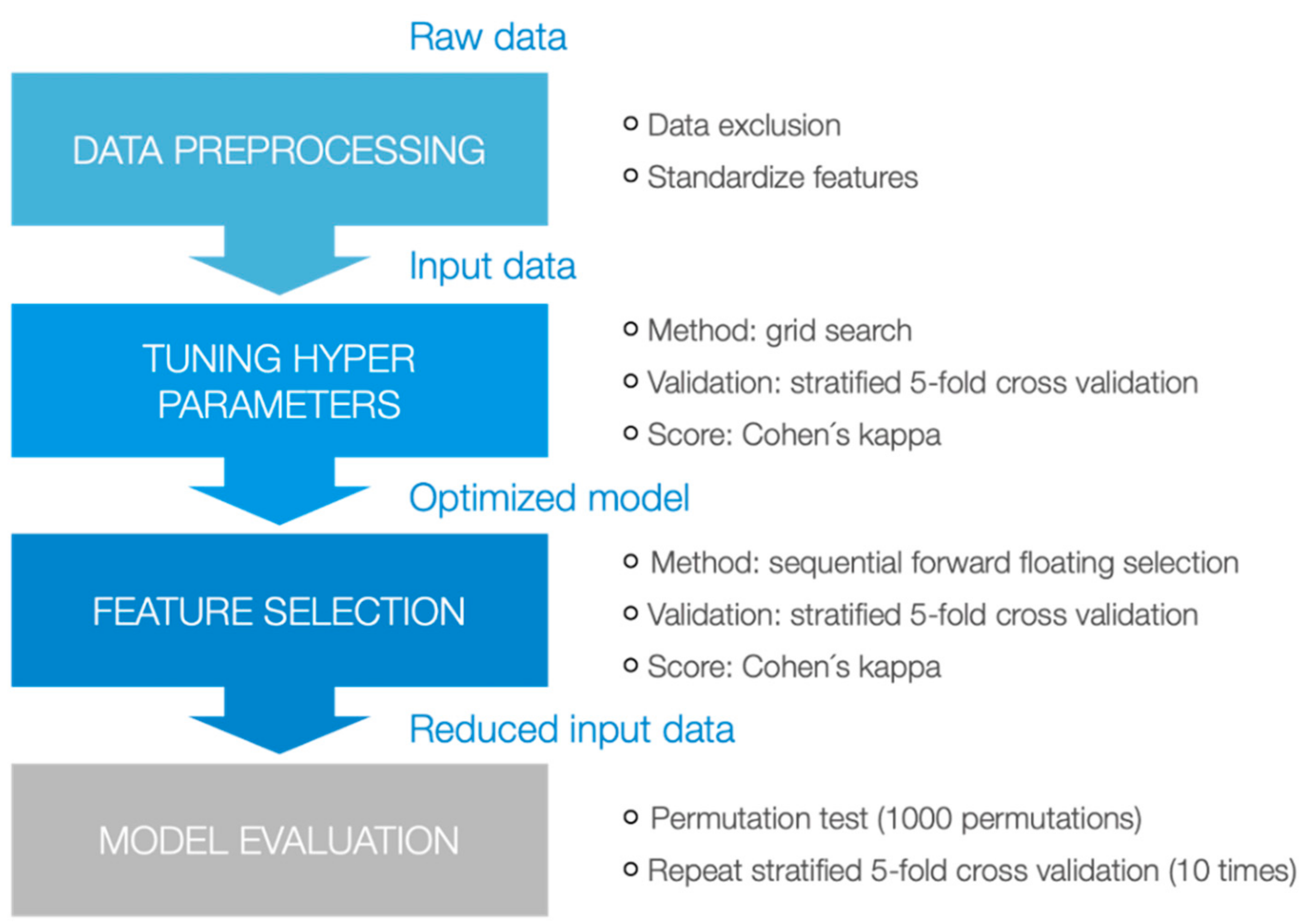
2.3. Machine Learning Approaches
3. Results
3.1. Descriptive Analyses
3.2. Machine Learning Techniques
4. Discussion
5. Conclusions
Author Contributions
Funding
Institutional Review Board Statement
Informed Consent Statement
Data Availability Statement
Conflicts of Interest
Appendix A

| Unmatched Set (N = 92) | Matched Set (N = 60) | |||||||
|---|---|---|---|---|---|---|---|---|
| MS (N = 54) | HC (N = 38) | p | MS (N = 30) | HC (N = 30) | p | |||
| Mean age in years (mean ± SD) | 40.3 ± 10.9 | 34.0 ± 13.3 | 0.002 b | 37.1 ± 12.5 | 36.9 ± 13.5 | 0.961 b | ||
| Gender | Female N (%) | 35 (64.8%) | 23 (60.5%) | 0.675 c | 21 (70.0%) | 21 (70.0%) | 0.999 c | |
| Male N (%) | 19 (35.2%) | 15 (39.5%) | 9 (30.0%) | 9 (30.0%) | ||||
| Duration of disease in years (mean ± SD) | 8.1 ± 6.0 | 7.1 ± 5.4 | ||||||
| EDSS (median) EDSS (Interquartile range) | 2 1.5–3.0 | 1.5 1.5–2.6 | ||||||
| Disease Course N (%) | RRMS | 52 (96.3%) | 29 (96.7%) | |||||
| PPMS | 2 (3.7%) | 1 (3.3%) | ||||||
| No. Features | Features | |
|---|---|---|
| DIERS data set | ||
| Gaussian Naive Bayes | 11 | COP-Deflection lateral R, Foot Rotation L, Foot Rotation R, Pre-Swing Phase R, Single Support L, Step Length L, Step Length R, Stride Length, Stride Time, Velocity, Walk Track anterior/posterior Position [SD] |
| Decision Tree | 1 | Velocity |
| k-Nearest Neighbor | 5 | Rearfoot L, Stance Phase R, Step Time L, Stride Length, Stride Time |
| SVM (linear kernel) | 28 | Bipedale Phase, Cadence, COP-Deflection lateral L, Foot Rotation L, Forefoot R, Loading Response L, Loading Response R, Midfoot L, Midfoot R, Pre-Swing Phase L, Pre-Swing Phase R, Rearfoot L, Rearfoot R, Single Support L, Single Support R, Stance Phase L, Stance Phase R, Step Length L, Step Length R, Step Time L, Step Width, Stride Length, Stride Time, Swing Phase L, Swing Phase R, Velocity, Walk Track anterior/posterior Position [SD], Walk Track lateral Position [SD] |
| SVM (rbf kernel) | 8 | Cadence, Foot Rotation L, Loading Response L, Pre-Swing Phase L, Single Support L, Step Length R, Velocity, Walk Track anterior/posterior Position [SD] |
| SVM (polynomial kernel) | 13 | COP-Deflection lateral L, Loading Response L, Midfoot L, Midfoot R, Pre-Swing Phase L, Rearfoot L, Single Support L, Stance Phase R, Step Length L, Step Length R, Stride Length, Stride Time, Swing Phase R |
| GAITRite data set | ||
| Gaussian Naive Bayes | 8 | Cycle Time Differential, Double Support Load Time R (%GC), HH Base Support L, Stance Time L, Step Extremity R, Step Time Differential, Stride Velocity L [SD], Swing Time L |
| Decision Tree | 3 | Stance Time L (%GC), Step Count, Swing Time R |
| k-Nearest Neighbor | 31 | Ambulation Time, Cadence, Cycle Time L, Distance, Double Supp. Time L (%GC), Double Supp. Time R (%GC), Double Supp. Time L [SD], Double Supp Time R [SD], Double Supp. Time L, Double Supp. Time R, Double Support Load Time L (%GC), Double Support Load Time L, Double Support Unload Time L (%GC), Double Support Unload Time R (%GC), Double Support Unload Time R, HH Base Support L, HH Base Support R, Single Supp. Time L (%GC), Single Supp. Time R (%GC), Stance Time L (%GC), Stance Time R [SD], Step Count, Step Extremity L, Step Extremity R, Step Length L [SD], Step Time L [SD], Step Time R [SD], Stride Time R [SD], Stride Velocity R, Swing Time L (%GC), Swing Time R |
| SVM (linear kernel) | 18 | Double Supp. Time L (%GC), Double Supp. Time R (%GC), Double Support Load Time L (%GC), Double Support Unload Time R (%GC), Double Support Unload Time R, Single Supp. Time L (%GC), Single Supp. Time R (%GC), Stance Time R (%GC), Stance Time L, Step Extremity R, Step Length L, Step Length R, Step Time Differential, Stride Length L [SD], Stride Length L, Stride Length R, Swing Time R (%GC), Swing Time R [SD] |
| SVM (rbf kernel) | 34 | Distance, Double Supp. Time L (%GC), Double Supp. Time R (%GC), Double Supp. Time R [SD], Double Supp. Time L, Double Supp. Time R, Double Support Load Time L (%GC), Double Support Load Time L, Double Support Load Time R, Double Support Unload Time L (%GC), Double Support Unload Time R (%GC), Double Support Unload Time R, Heel Off On Perc R, HH Base Support L, HH Base Support R, Single Supp. Time L (%GC), Single Supp. Time R (%GC), Stance Time L (%GC), Stance Time R (%GC), Step Count, Step Length Differential, Step Length L, Step Length R, Step Time Differential, Stride Length L [SD], Stride Length L, Stride Length R, Stride Velocity L, HH Base Support R [SD], Swing Time L (%GC), Swing Time R (%GC), Swing Time R, Toe In / Out R, Velocity |
| SVM (polynomial kernel) | 10 | Distance, Double Supp. Time L, Double Support Unload Time L (%GC) L, Heel Off On Perc R, Heel Off On L [SD], Step Time Differential, Stride Velocity L, Stride Velocity L [SD], Swing Time L, Toe In / Out R |
| Mobility Lab data set | ||
| Gaussian Naive Bayes | 15 | Lower Limb—Double Support L (%GCT), Lower Limb—Double Support R (%GCT), Lower Limb—Foot Strike Angle R, Lower Limb—Stance R (%GCT), Lower Limb—Terminal Double Support R (%GCT) [SD], Lower Limb—Toe Off Angle L, Lower Limb—Toe Off Angle R, Lumbar—Sagittal Range of Motion, Trunk—Coronal Range of Motion [SD], Trunk—Sagittal Range of Motion, Trunk—Transverse Range of Motion, Turns—N, Turns—Steps in Turn, Turns—Turn Velocity, Upper Limb—Arm Range of Motion L |
| Decision Tree | 41 | Duration, Lower Limb—Cadence L, Lower Limb—Cadence R, Lower Limb—Circumduction L, Lower Limb—Circumduction L [SD], Lower Limb—Circumduction R, Lower Limb—Elevation at Midswing L, Lower Limb—Elevation at Midswing R, Lower Limb—Elevation at Midswing R [SD], Lower Limb—Foot Strike Angle L, Lower Limb—Foot Strike Angle L [SD], Lower Limb—Foot Strike Angle R, Lower Limb—Foot Strike Angle R [SD], Lower Limb—Gait Cycle Duration L, Lower Limb—Gait Cycle Duration L [SD], Lower Limb—Gait Cycle Duration R, Lower Limb—Gait Cycle Duration R [SD], Lower Limb—Gait Speed L, Lower Limb—Gait Speed R, Lower Limb—Lateral Step Variability L, Lower Limb—Lateral Step Variability R, Lower Limb—N, Lower Limb—Single Limb Support L (%GCT) [SD], Lower Limb—Stance L (%GCT), Lower Limb—Stance L (%GCT) [SD], Lower Limb—Stance R (%GCT) [SD], Lower Limb—Step Duration L, Lower Limb—Step Duration L [SD], Lower Limb—Step Duration R, Lower Limb—Step Duration R [SD], Lower Limb—Stride Length L, Lower Limb—Stride Length L [SD], Lower Limb—Toe Off Angle L, Lower Limb—Toe Off Angle L [SD], Lower Limb—Toe Off Angle R, Lower Limb—Toe Off Angle R [SD], Lower Limb—Toe Out Angle L, Lower Limb—Toe Out Angle L [SD], Lower Limb—Toe Out Angle R, Trunk—Transverse Range of Motion [SD], Turns—Steps in Turn [SD] |
| k-Nearest Neighbor | 9 | Lower Limb—Gait Cycle Duration L, Lower Limb—Single Limb Support R (%GCT), Lower Limb—Terminal Double Support R (%GCT), Lower Limb—Terminal Double Support R (%GCT) [SD], Lower Limb—Toe Off Angle L [SD], Lower Limb—Toe Off Angle R [SD], Lumbar—Coronal Range of Motion, Trunk—Coronal Range of Motion, Upper Limb—Arm Range of Motion L [SD] |
| SVM (linear kernel) | 5 | Lower Limb—Stride Length R, Lower Limb—Toe Off Angle R [SD], Lumbar—Transverse Range of Motion, Lumbar—Transverse Range of Motion [SD], Upper Limb—Arm Range of Motion R [SD] |
| SVM (rbf kernel) | 24 | Lower Limb—Double Support R (%GCT), Lower Limb—Foot Strike Angle R [SD], Lower Limb—Gait Speed L, Lower Limb—Gait Speed R, Lower Limb—Lateral Step Variability L, Lower Limb—Single Limb Support R (%GCT), Lower Limb—Stance L (%GCT), Lower Limb—Stride Length L, Lower Limb—Terminal Double Support R (%GCT), Lower Limb—Toe Off Angle L, Lower Limb—Toe Off Angle L [SD], Lower Limb—Toe Off Angle R, Lower Limb—Toe Off Angle R [SD], Lower Limb—Toe Out Angle R [SD], Lumbar—Coronal Range of Motion [SD], Lumbar—Sagittal Range of Motion, Lumbar—Sagittal Range of Motion [SD], Trunk—Coronal Range of Motion [SD], Trunk—Transverse Range of Motion [SD], Turns—Turn Velocity [SD], Upper Limb—Arm Range of Motion L, Upper Limb—Arm Range of Motion L [SD], Upper Limb—Arm Swing Velocity L [SD], Upper Limb—Arm Swing Velocity R [SD] |
| SVM (polynomial kernel) | 12 | Lower Limb—Circumduction R, Lower Limb—Elevation at Midswing R, Lower Limb—Foot Strike Angle L, Lower Limb—Foot Strike Angle R, Lower Limb—Gait Speed L, Lower Limb—Stride Length L, Lower Limb—Toe Off Angle L, Lower Limb—Toe Off Angle L [SD], Turns—Angle [SD], Upper Limb—Arm Range of Motion R, Upper Limb—Arm Range of Motion R [SD], Upper Limb—Arm Swing Velocity L |
References
- Goldenberg, M.M. Multiple Sclerosis Review. Pharm. Ther. 2012, 37, 175. [Google Scholar]
- Ziemssen, T. Symptom Management in Patients with Multiple Sclerosis. J. Neurol. Sci. 2011, 311, S48–S52. [Google Scholar] [CrossRef]
- Galea, M.P.; Cofré Lizama, L.E.; Butzkueven, H.; Kilpatrick, T.J. Gait and Balance Deterioration Over a 12-Month Period in Multiple Sclerosis Patients with EDSS Scores ≤ 3.0. Neuro Rehabil. 2017, 40, 277–284. [Google Scholar] [CrossRef]
- Filli, L.; Sutter, T.; Easthope, C.S.; Killeen, T.; Meyer, C.; Reuter, K.; Lorincz, L.; Bolliger, M.; Weller, M.; Curt, A.; et al. Profiling Walking Dysfunction in Multiple Sclerosis: Characterisation, Classification and Progression Over Time. Sci. Rep. 2018, 8, 1–13. [Google Scholar] [CrossRef]
- LaRocca, N.G. Impact of Walking Impairment in Multiple Sclerosis. Patient Patient-Cent. Outcomes Res. 2011, 4, 189–201. [Google Scholar] [CrossRef] [PubMed]
- Kalron, A.; Givon, U. Gait Characteristics According to Pyramidal, Sensory and Cerebellar EDSS Subcategories in People with Multiple Sclerosis. J. Neurol. 2016, 263, 1796–1801. [Google Scholar] [CrossRef] [PubMed]
- Novotna, K.; Sobisek, L.; Horakova, D.; Havrdova, E.; Lizrova Preiningerova, J. Quantification of Gait Abnormalities in Healthy-Looking Multiple Sclerosis Patients (with Expanded Disability Status Scale 0–1.5). Eur. Neurol. 2016, 76, 99–104. [Google Scholar] [CrossRef]
- Benedetti, M.G.; Piperno, R.; Simoncini, L.; Bonato, P.; Tonini, A.; Giannini, S. Gait Abnormalities in Minimally Impaired Multiple Sclerosis Patients. Mult. Scler. Int. 1999, 5, 363–368. [Google Scholar] [CrossRef] [PubMed]
- Martin, C.L.; Phillips, B.A.; Kilpatrick, T.J.; Butzkueven, H.; Tubridy, N.; McDonald, E. Gait and Balance Impairment in Early Multiple Sclerosis in The Absence of Clinical Disability. Mult. Scler. J. 2006, 12, 620–628. [Google Scholar] [CrossRef] [PubMed]
- Wiendl, H.; Meuth, S.G. Pharmacological Approaches to Delaying Disability Progression in Patients with Multiple Sclerosis. Drugs 2015, 75, 947–977. [Google Scholar] [CrossRef] [PubMed] [Green Version]
- Voigt, I.; Ziemssen, T. Internationale “Brain Health Initiative” und Multiple Sklerose. DG Neurol. 2019, 3, 1–7. [Google Scholar] [CrossRef]
- Ziemssen, T.; Kern, R.; Thomas, K. Multiple Sclerosis: Clinical Profiling and Data Collection as Prerequisite for Personalized Medicine Approach. BMC Neurol. 2016, 16, 124. [Google Scholar] [CrossRef] [Green Version]
- Ziemssen, T.; Piani-Meier, D.; Bennett, B.; Johnson, C.; Tinsley, K.; Trigg, A.; Hach, T.; Dahlke, F.; Tomic, D.; Tolley, C.; et al. A Physician-Completed Digital Tool for Evaluating Disease Progression (Multiple Sclerosis Progression Discussion Tool): Validation Study. J. Med. Internet Res. 2020, 22, e16932. [Google Scholar] [CrossRef]
- Inojosa, H.; Proschmann, U.; Akgün, K.; Ziemssen, T. Should We Use Clinical Tools to Identify Disease Progression? Front. Neurol. 2021, 11, 1890. [Google Scholar] [CrossRef]
- Voigt, I.; Gabriel, H.; Castro, I.; Dillenseger, A.; Haase, R. Digital Twins for Multiple Sclerosis. Front. Immunol. 2021, 12, 1556. [Google Scholar] [CrossRef] [PubMed]
- Shanahan, C.J.; Boonstra, F.M.C.; Cofré Lizama, L.E.; Strik, M.; Moffat, B.A.; Khan, F.; Kilpatrick, T.J.; van der Walt, A.; Galea, M.P.; Scott, C.K. Technologies for Advanced Gait and Balance Assessments in People with Multiple Sclerosis. Front. Neurol. 2018, 8, 708. [Google Scholar] [CrossRef] [PubMed] [Green Version]
- Inojosa, H.; Schriefer, D.; Ziemssen, T. Clinical Outcome Measures in Multiple Sclerosis: A Review. Autoimmun. Rev. 2020, 19, 102512. [Google Scholar] [CrossRef]
- Hora, M.; Soumar, L.; Pontzer, H.; Sládek, V. Body Size and Lower Limb Posture during Walking in Humans. PLoS ONE 2017, 12, 1–26. [Google Scholar] [CrossRef] [PubMed]
- Pau, M.; Corona, F.; Pilloni, G.; Porta, M.; Coghe, G.; Cocco, E. Do Gait Patterns Differ in Men and Women with Multiple Sclerosis? Mult. Scler. Relat. Disord. 2017, 18, 202–208. [Google Scholar] [CrossRef]
- Tenforde, A.S.; Borgstrom, H.E.; Outerleys, J.; Davis, I.S. Is Cadence Related to Leg Length and Load Rate? J. Orthop. Sports Phys. Ther. 2019, 49, 280–283. [Google Scholar] [CrossRef]
- Vienne-Jumeau, A.; Quijoux, F.; Vidal, P.P.; Ricard, D. Value of Gait Analysis for Measuring Disease Severity using Inertial Sensors in Patients with Multiple Sclerosis: Protocol for A Systematic Review and Meta-Analysis. Syst. Rev. 2019, 8, 1–5. [Google Scholar] [CrossRef] [PubMed]
- Scholz, M.; Haase, R.; Schriefer, D.; Voigt, I.; Ziemssen, T. Electronic Health Interventions in The Case of Multiple Sclerosis: From Theory to Practice. Brain Sci. 2021, 11, 180. [Google Scholar] [CrossRef] [PubMed]
- Liparoti, M.; Della Corte, M.; Rucco, R.; Sorrentino, P.; Sparaco, M.; Capuano, R.; Minino, R.; Lavorgna, L.; Agosti, V.; Sorrentino, G.; et al. Gait Abnormalities in Minimally Disabled People with Multiple Sclerosis: A 3D-Motion Analysis Study. Mult. Scler. Relat. Disord. 2019, 29, 100–107. [Google Scholar] [CrossRef]
- Saxe, R.C.; Kappagoda, S.; Mordecai, D.K.A. Classification of Pathological and Normal Gait: A Survey. arXiv 2020, arXiv:2012.14465. [Google Scholar]
- Santinelli, F.B.; Sebastião, E.; Kuroda, M.H.; Moreno, V.C.; Pilon, J.; Vieira, L.H.P.; Barbieri, F.A. Cortical Activity and Gait Parameter Characteristics in People with Multiple Sclerosis During Unobstructed Gait and Obstacle Avoidance. Gait Posture 2021, 86, 226–232. [Google Scholar] [CrossRef]
- Tajali, S.; Mehravar, M.; Negahban, H.; van Dieën, J.H.; Shaterzadeh-Yazdi, M.-J.; Mofateh, R. Impaired Local Dynamic Stability During Treadmill Walking Predicts Future Falls in Patients with Multiple Sclerosis_ A Prospective Cohort Study. Clin. Biomech. 2019, 67, 197–201. [Google Scholar] [CrossRef] [Green Version]
- Scholz, M.; Haase, R.; Trentzsch, K.; Stölzer-Hutsch, H.; Ziemssen, T. Improving Digital Patient Care: Lessons Learned from Patient-Reported and Expert-Reported Experience Measures for the Clinical Practice of Multidimensional Walking Assessment. Brain Sci. 2021, 11, 786. [Google Scholar] [CrossRef] [PubMed]
- Dilsizian, S.E.; Siegel, E.L. Artificial Intelligence in Medicine and Cardiac Imaging: Harnessing Big Data and Advanced Computing to Provide Personalized Medical Diagnosis and Treatment. Curr. Cardiol. Rep. 2014, 16, 441. [Google Scholar] [CrossRef]
- Jiang, F.; Jiang, Y.; Zhi, H.; Dong, Y.; Li, H.; Ma, S.; Wang, Y.; Dong, Q.; Shen, H.; Wang, Y. Artificial Intelligence in Healthcare: Past, Present and Future. Stroke Vasc. Neurol. 2017, 2. [Google Scholar] [CrossRef]
- Piryonesi, S.M.; Rostampour, S.; Piryonesi, S.A. Predicting Falls and Injuries in People with Multiple Sclerosis using Machine Learning Algorithms. Mult. Scler. Relat. Disord. 2021, 49, 102740. [Google Scholar] [CrossRef] [PubMed]
- Ravi, D.; Wong, C.; Deligianni, F.; Berthelot, M.; Andreu-perez, J.; Lo, B. Deep Learning for Health Informatics. IEEE J. Biomed. Health Inform. 2017, 21, 4–21. [Google Scholar] [CrossRef] [Green Version]
- Gulshan, V.; Peng, L.; Coram, M.; Stumpe, M.C.; Wu, D.; Narayanaswamy, A.; Venugopalan, S.; Widner, K.; Madams, T.; Cuadros, J.; et al. Development and Validation of a Deep Learning Algorithm for Detection of Diabetic Retinopathy in Retinal Fundus Photographs. JAMA J. Am. Med. Assoc. 2016, 316, 2402–2410. [Google Scholar] [CrossRef]
- Trentzsch, K.; Weidemann, M.L.; Torp, C.; Inojosa, H.; Scholz, M.; Haase, R.; Schriefer, D.; Akgun, K.; Ziemssen, T. The Dresden Protocol for Multidimensional Walking Assessment (DMWA) in Clinical Practice. Front. Neurosci. 2020, 14. [Google Scholar] [CrossRef]
- McDonough, A.L.; Batavia, M.; Chen, F.C.; Kwon, S.; Ziai, J. The Validity and Reliability of the GAITRite System’s Measurements: A Preliminary Evaluation. Arch. Phys. Med. Rehabil. 2001, 82, 419–425. [Google Scholar] [CrossRef] [Green Version]
- Bilney, B.; Morris, M.; Webster, K. Concurrent Related Validity of the GAITRite® Walkway System for Quantification of The Spatial and Temporal Parameters of Gait. Gait Posture 2003, 17, 68–74. [Google Scholar] [CrossRef]
- Webster, K.E.; Wittwer, J.E.; Feller, J.A. Validity of the GAITRite® Walkway System for The Measurement of Averaged and Individual Step Parameters of Gait. Gait Posture 2005, 22, 317–321. [Google Scholar] [CrossRef]
- Electronic Gaitr. GAITRite Electronic Walkway Technical Reference. Tech. Ref. 2013, 1–50. Available online: https://www.procarebv.nl/wp-content/uploads/2017/01/Technische-aspecten-GAITrite-Walkway-System.pdf (accessed on 5 June 2021).
- Mancini, M.; King, L.; Salarian, A.; Holmstrom, L.; McNames, J.; Horak, F.B. Mobility Lab to Assess Balance and Gait with Synchronized Body-worn Sensors. J. Bioeng. Biomed. Sci. 2011, 7. [Google Scholar] [CrossRef]
- Schmitz-Hübsch, T.; Brandt, A.U.; Pfueller, C.; Zange, L.; Seidel, A.; Kühn, A.A.; Friedermann, P.; Minnerop, M.; Doss, S. Accuracy and Repeatability of Two Methods of Gait Analysis-GaitRiteTM und Mobility LabTM-in Subjects with Cerebellar Ataxia. Gait Posture 2016, 48, 194–201. [Google Scholar] [CrossRef] [PubMed]
- Solomon, A.J.; Jacobs, J.V.; Lomond, K.V.; Henry, S.M. Detection of Postural Sway Abnormalities by Wireless Inertial Sensors in Minimally Disabled Patients with Multiple Sclerosis: A Case-Control Study. J. Neuroeng. Rehabil. 2015, 12, 1–9. [Google Scholar] [CrossRef] [PubMed] [Green Version]
- APDM Inc. Wearable Technologies. In User Guide Mobility Lab; APDM Inc.: Portland, OR, USA, 2020. [Google Scholar]
- Spain, R.; St George, R.; Salarian, A.; Mancini, M.; Wagner, J.M.; Horak, F.B.; Bourdette, D. Body-Worn Motion Sensors Detect Balance and Gait Deficits in People with Multiple Sclerosis Who Have Normal Walking Speed. Gait Posture 2012, 35, 573–578. [Google Scholar] [CrossRef] [PubMed] [Green Version]
- Mancini, M.; Horak, F.B. Potential of APDM Mobility Lab for The Monitoring of The Progression of Parkinson’s Disease. Expert Rev. Med. Devices 2016, 13, 455–462. [Google Scholar] [CrossRef] [PubMed]
- Mancini, M.; Salarian, A.; Carlson-Kuhta, P.; Zampieri, C.; King, L.; Chiari, L.; Horak, F.B. ISway: A Sensitive, Valid and Reliable Measure of Postural Control. J. Neuroeng. Rehabil. 2012, 9, 1. [Google Scholar] [CrossRef] [Green Version]
- Killeen, T.; Elshehabi, M.; Filli, L.; Hobert, M.A.; Hansen, C.; Rieger, D.; Brockmann, K.; Nussbaum, S.; Zörner, B.; Bolliger, M.; et al. Arm Swing Asymmetry in Overground Walking. Sci. Rep. 2018, 8, 1–10. [Google Scholar] [CrossRef]
- Washabaugh, E.P.; Kalyanaraman, T.; Adamczyk, P.G.; Claflin, E.S.; Krishnan, C. Validity and Repeatability of Inertial Measurement Units for Measuring Gait Parameters. Gait Posture 2017, 55, 87–93. [Google Scholar] [CrossRef] [Green Version]
- Werner, C.; Heldmann, P.; Hummel, S.; Bauknecht, L.; Bauer, J.M.; Hauer, K. Concurrent Validity, Test-Retest Reliability, and Sensitivity to Change of a Single Body-Fixed Sensor for Gait Analysis During Rollator-Assisted Walking in Acute Geriatric Patients. Sensors 2020, 20, 4866. [Google Scholar] [CrossRef] [PubMed]
- Cooper, K.H. A Means of Assessing Maximal Oxygen Intake. JAMA 1968, 203, 135–138. [Google Scholar] [CrossRef]
- Butland, R.J.A.; Pang, J.; Gross, E.R.; Woodcock, A.A.; Geddes, D.M. Two-, Six-, and 12-Minute Walking Tests in Respiratory Disease. Br. Med. J. 1982, 284, 1607–1608. [Google Scholar] [CrossRef] [Green Version]
- Goldman, M.D.; Marrie, R.A.; Cohen, J.A. Evaluation of The Six-Minute Walk in Multiple Sclerosis Subjects and Healthy Controls. Mult. Scler. 2008, 14, 383–390. [Google Scholar] [CrossRef]
- Brooks, D.; Parsons, J.; Tran, D.; Jeng, B.; Gorczyca, B.; Newton, J.; Lo, V.; Dear, C.; Silaj, E.; Hawn, T. The Two-Minute Walk Test as a Measure of Functional Capacity in Cardiac Surgery Patients. Arch. Phys. Med. Rehabil. 2004, 85, 1525–1530. [Google Scholar] [CrossRef]
- Gijbels, D.; Eijnde, B.O.; Feys, P. Comparison of the 2- and 6-Minute Walk Test in Multiple Sclerosis. Mult. Scler. 2011, 17, 1269–1272. [Google Scholar] [CrossRef]
- Rossier, P.; Wade, D.T. Validity and Reliability Comparison of 4 Mobility Measures in Patients Presenting with Neurologic Impairment. Arch. Phys. Med. Rehabil. 2001, 82, 9–13. [Google Scholar] [CrossRef]
- Scalzitti, D.A.; Harwood, K.J.; Maring, J.R.; Leach, S.J.; Ruckert, E.A.; Costello, E. Validation of the 2-Minute Walk Test with the 6-Minute Walk Test and Other Functional Measures in Persons with Multiple Sclerosis. Int. J. MS Care 2018, 20, 158–163. [Google Scholar] [CrossRef] [Green Version]
- Degenhardt, B.F.; Starks, Z.; Bhatia, S. Reliability of the DIERS Formetric 4D Spine Shape Parameters in Adults without Postural Deformities. Biomed. Res. Int. 2020, 2020, 1796247. [Google Scholar] [CrossRef] [PubMed]
- Liu, X.; Yang, X.S.; Wang, L.; Yu, M.; Liu, X.G.; Liu, Z.J. Usefulness of a Combined Approach of DIERS Formetric 4D® and QUINTIC Gait Analysis System to Evaluate the Clinical Effects of Different Spinal Diseases on Spinal-Pelvic-Lower Limb Motor Function. J. Orthop. Sci. 2020, 25, 576–581. [Google Scholar] [CrossRef]
- Tabard-Fougère, A.; Bonnefoy-Mazure, A.; Hanquinet, S.; Lascombes, P.; Armand, S.; Dayer, R. Validity and Reliability of Spine Rasterstereography in Patients with Adolescent Idiopathic Scoliosis. Spine 2017, 42, 98–105. [Google Scholar] [CrossRef]
- Hübner, S. Manual DIERS Products; DIERS International GmbH: Schlangenbad, Germany, 2021; pp. 1–50. [Google Scholar]
- Hobart, J.C.; Riazi, A.; Lamping, D.L.; Fitzpatrick, R.; Thompson, A.J. Measuring the Impact of MS on Walking Ability: The 12-Item MS Walking Scale (MSWS-12). Neurology 2003, 60, 31–36. [Google Scholar] [CrossRef] [PubMed]
- Ziemssen, T.; Phillips, G.; Shah, R.; Mathias, A.; Foley, C.; Coon, C.; Sen, R.; Lee, A.; Agarwal, S. Development of the Multiple Sclerosis (MS) Early Mobility Impairment Questionnaire (EMIQ). J. Neurol. 2016, 263, 1969–1983. [Google Scholar] [CrossRef] [PubMed]
- D’Amico, E.; Haase, R.; Ziemssen, T. Review: Patient-Reported Outcomes in Multiple Sclerosis Care. Mult. Scler. Relat. Disord. 2019. [Google Scholar] [CrossRef]
- Landis, J.R.; Koch, G.G. The Measurement of Observer Agreement for Categorical Data. Biometrics 1977, 33, 159–174. [Google Scholar] [CrossRef] [PubMed] [Green Version]
- Sagi, O.; Rokach, L. Ensemble Learning: A Survey. Wiley Interdiscip. Rev. Data Min. Knowl. Discov. 2018, 8, e1249. [Google Scholar] [CrossRef]
- Webb, G.I.; Zheng, Z. Multistrategy Ensemble Learning: Reducing Error by Combining Ensemble Learning Techniques. IEEE Trans. Knowl. Data Eng. 2004, 16, 980–991. [Google Scholar] [CrossRef] [Green Version]
- Tang, S.; Zheng, Y.T.; Wang, Y.; Chua, T.S. Sparse Ensemble Learning for Concept Detection. IEEE Trans. Multimed. 2012, 14, 43–54. [Google Scholar] [CrossRef]
- Pudil, P.; Novovieova, J.; Kittler, J. Floating Search Methods in Feature Selection. Pattern Recognit. Lett. 1994, 15, 1119–1125. [Google Scholar] [CrossRef]
- Ojala, M.; Garriga, G.C. Permutation Tests for Studying Classifier Performance. J. Mach. Learn. Res. 2010, 11, 1833–1863. [Google Scholar]
- Pedregosa, F.; Varoquaux, G.; Gramfort, A.; Michel, V.; Thirion, B.; Grisel, O. Scikit-learn: Machine learning in Python. J. Mach. Learn. Res. 2011, 12, 2825–2830. [Google Scholar]
- Raschka, S. MLxtend: Providing Machine Learning and Data Science Utilities and Extensions to Python’s Scientific Computing Stack. J. Open Source Softw. 2018, 3, 638. [Google Scholar] [CrossRef]
- Chee, J.N.; Ye, B.; Gregor, S.; Berbrayer, D.; Mihailidis, A.; Patterson, K.K. Influence of Multiple Sclerosis on Spatiotemporal Gait Parameters: A Systematic Review and Meta-Regression. Arch. Phys. Med. Rehabil. 2021. [Google Scholar] [CrossRef] [PubMed]
- Plotnik, M.; Wagner, J.M.; Adusumilli, G.; Gottlieb, A.; Naismith, R.T. Gait Asymmetry, and Bilateral Coordination of Gait during a Six-Minute Walk Test in Persons with Multiple Sclerosis. Sci. Rep. 2020, 10, 1–11. [Google Scholar] [CrossRef] [PubMed]
- Wu, X.; Kumar, V.; Ross, Q.J.; Ghosh, J.; Yang, Q.; Motoda, H.; McLachlan, G.J.; Ng, A.; Liu, B.; Yu, P.S.; et al. Top 10 Algorithms in Data Mining. Knowl. Inf. Syst. 2008, 14, 1–37. [Google Scholar] [CrossRef] [Green Version]
- Domingos, P.; Pazzani, M. On the Optimality of the Simple Bayesian Classifier under Zero-One Loss. Machine Learning. Mach. Learn. 1997, 29, 103–130. [Google Scholar] [CrossRef]
- Hand, D.J.; Yu, K. Idiot’s Bayes-Not So Stupid After All? Int. Stat. Rev. 2001, 69, 385–398. [Google Scholar] [CrossRef]
- Russek, E.; Richard, A.; Fisher, K.D.; Fisher, L. The Effect of Assuming Independence in Applying Bayes’ Theorem to Risk Estimation and Classification in Diagnosis *. Comput. Biomed. Res. 1983, 16, 537–552. [Google Scholar] [CrossRef]
- Kotsiantis, S.B. Supervised Machine Learning: A Review of Classification Techniques. Emerg. Artif. Intell. Appl. Comput. Eng. 2007, 160, 249–268. [Google Scholar] [CrossRef]
- Murthy, S.K. Automatic Construction of Decision Trees from Data: A Multi-Disciplinary Survey. Data Min. Knowl. Discov. 1998, 2, 345–389. [Google Scholar] [CrossRef]
- Quinlan, J.R. Induction of Decision Trees. Mach. Learn. 1986, 1, 81–106. [Google Scholar] [CrossRef] [Green Version]
- Schaffer, C. Overfitting Avoidance as Bias. Mach. Learn. 1993, 10, 153–178. [Google Scholar] [CrossRef] [Green Version]
- Cost, S.; Salzberg, S. A Weighted Nearest Neighbor Algorithm for Learning with Symbolic Features. Mach. Learn. 1993, 10, 57–78. [Google Scholar] [CrossRef]
- Wettschereck, D.; Aha, D.W.; Mohri, T. A Review and Empirical Evaluation of Feature Weighting Methods for a Class of Lazy Learning Algorithms. Artif. Intell. Rev. 1997, 11, 273–314. [Google Scholar] [CrossRef]
- Sánchez, V.D.A. Advanced Support Vector Machines and Kernel Methods. Neurocomputing 2003, 55, 5–20. [Google Scholar] [CrossRef]
- Joachims, T. Text Categorization with SVM: Learning with Many Relevant Features. Eur. Conf. Mach. Learn. Springer Berl. 2009, 4, 137–142. [Google Scholar] [CrossRef] [Green Version]
- Burges, C.J.C. A Tutorial on Support Vector Machines for Pattern Recognition. Data Min. Knowl. Discov. 1998, 2, 121–167. [Google Scholar] [CrossRef]
- Bohannon, R.W. Normative Reference Values for The Two-Minute Walk Test Derived by Meta-Analysis. J. Phys. Ther. Sci. 2017, 29, 2224–2227. [Google Scholar] [CrossRef] [PubMed] [Green Version]
- Wolf, I.; Bridenbaugh, S.A.; Gschwind, Y.J.; Kressig, R.W. Gangveränderungen und Sturzrisiko. Prax. Verl. Hans Huber 2012, 101, 175–181. [Google Scholar] [CrossRef] [PubMed]
- Oh-Park, M.; Holtzer, R.; Xue, X.; Verghese, J. Conventional and Robust Quantitative Gait Norms in Community-Dwelling Older Adults. J. Am. Geriatr. Soc. 2010, 58, 1512–1518. [Google Scholar] [CrossRef] [Green Version]
- Duan, K.; Keerthi, S.; Poo, A. Evaluation of Simple Performance Measures for Tuning SVM Hyperparameters. Neurocomputing 2003, 51, 41–59. [Google Scholar] [CrossRef]
- Wolpert, D.H. On Overfitting Avoidance as Bias; Technical Report SFI TR 92-03-5001; The Santa Fe Institute: Santa Fe, NM, USA, 1993. [Google Scholar]
- Gu, X.; Guo, Y.; Deligianni, F.; Lo, B.; Yang, G.-Z. Cross-Subject and Cross-Modal Transfer for Generalized Abnormal Gait Pattern Recognition. IEEE Trans. Neural Netw. Learn Syst. 2020, 32, 546–560. [Google Scholar] [CrossRef] [PubMed]
| DIERS | GAITRite | Mobility Lab |
|---|---|---|
| Bipedale Phase (%GCT) [mean] | Ambulation Time (s) [mean] | Duration (s) |
| Cadence (steps/min) [mean] | Cadence (steps/min) [mean] | Lower Limb—Cadence L/R (steps/min) [mean]/[SD] |
| COP-Deflection lateral L/R (cm) [mean] | Cycle Time Differential (s) | Lower Limb—Circumduction L/R (cm) [mean]/[SD] |
| Distance (cm) [mean] | Cycle Time L/R (s) [mean] | Lower Limb—Double Support L/R (%GCT) [mean]/[SD] |
| Foot Rotation L/R (degrees) [mean] | Distance (cm) [mean] | Lower Limb—Elevation at Midswing L/R (cm) [mean]/[SD] |
| Forefoot L/R (% Stance Phase) [mean] | Double Supp. Time L/R (s)/(%GCT) [mean]/[SD] | Lower Limb—Foot Strike Angle L/R (degrees) [mean]/[SD] |
| Loading Response L/R (%GCT) [mean] | Double Support Load Time L/R (s)/ (%GCT) [mean] | Lower Limb—Gait Cycle Duration L/R (s) [mean]/[SD] |
| Midfoot L/R (% Stance Phase) [mean] | Double Support Unload Time L/R (s)/(%GCT) [mean] | Lower Limb—Gait Speed L/R (m/s) [mean]/[SD] |
| Pre-Swing Phase L/R (%GCT) [mean] | Functional Amb. Profile ( ) | Lower Limb—Lateral Step Variability L/R (cm) |
| Rearfoot L/R (% Stance Phase) [mean] | Heel Off On Perc L/R (s) [mean] | Lower Limb—N (#) |
| Single Support L/R (%GCT) [mean] | Heel Off On Time L/R (s) [mean]/[SD] | Lower Limb—Single Limb Support L/R (%GCT) [mean]/[SD] |
| Stance Phase L/R (%GCT) [mean] | HH-Base Support L/R (cm) [mean]/[SD] | Lower Limb—Stance L/R (%GCT) [mean]/[SD] |
| Step Length L/R (cm) [mean] | Normalized Velocity (cm/s) [mean] | Lower Limb—Step Duration L/R (s) [mean]/[SD] |
| Step Time L/R (ms) [mean] | Single Supp. Time L/R (s)/(%GCT) [mean]/[SD] | Lower Limb—Stride Length L/R (m) [mean]/[SD] |
| Step Width (cm) [mean] | Stance Time L/R (s)/(%GCT) [mean]/[SD] | Lower Limb—Swing L/R (%GCT) [mean]/[SD] |
| Stride Length (cm) [mean] | Step Count ( ) | Lower Limb—Terminal Double Support L/R (%GCT) [mean]/[SD] |
| Stride Time (ms) [mean] | Step Extremity L/R (ratio) | Lower Limb—Toe Off Angle L/R (degrees) [mean]/[SD] |
| Swing Phase L/R (%GCT) [mean] | Step Length Differential (cm) | Lower Limb—Toe Out Angle L/R (degrees) [mean]/[SD] |
| Velocity (km/h) [mean] | Step Length L/R (cm) [mean]/[SD] | Lumbar/Trunk—Coronal Range of Motion (degrees) [mean]/[SD] |
| Walk Track anterior/posterior Position (mm) [SD] | Step Time Differential (s) | Lumbar/Trunk—Sagittal Range of Motion (degrees) [mean]/[SD] |
| Walk Track lateral Position (mm) [SD] | Step Time L/R (s) [mean]/[SD] | Lumbar/Trunk—Transverse Range of Motion (degrees) [mean]/[SD] |
| Stride Length L/R (cm) [mean]/[SD] | Turns—Angle (degrees) [mean]/[SD] | |
| Stride Time L/R (s) [SD] | Turns—Duration (s) [mean]/[SD] | |
| Stride Velocity L/R (cm/s) [mean]/[SD] | Turns—N ( ) | |
| Swing Time L/R (s)/(%GCT) [mean]/[SD] | Turns—Steps in Turn ( ) [mean]/[SD] | |
| Toe In/Out L/R (degrees) [mean] | Turns—Turn Velocity (degrees/s) [mean]/[SD] | |
| Velocity (cm/s) [mean] | Upper Limb—Arm Range of Motion L/R (degrees) [mean]/[SD] | |
| Upper Limb—Arm Swing Velocity L/R (degrees/s) [mean]/[SD] |
| Method | Hyperparameter | Min | Max | Step Size | Scale |
|---|---|---|---|---|---|
| Decision Tree | Criterion: ‘gini’ or ‘entropy’ | - | - | - | - |
| Maximum depth | 2 | 7 | 1 | linear | |
| Minimum samples at a leaf node | 5 | 20 | 1 | linear | |
| k-Nearest Neighbor | Weights: ‘uniform’ or ‘distance’ | - | - | - | - |
| Distance metric: ‘euclidean’ or ‘manhattan’ | - | - | - | - | |
| Numbers of neighbors k | 2 | 22 | 1 | linear | |
| SVM (linear kernel) | Regularization C | 0.01 | 10 | 10 | logarithmic |
| SVM (rbf kernel) | Regularization C | 1 | 10 | 1 | linear |
| Kernel coefficient gamma | 0.01 | 0.1 | 0.01 | linear | |
| SVM (polynomial kernel) | Regularization C | 0.1 | 10 | 10 | logarithmic |
| Kernel coefficient gamma | 0.01 | 0.1 | 0.01 | linear | |
| Degree | 1 | 10 | 1 | linear |
| Outcome Variable | MS (N = 30) | HC (N = 30) | p |
|---|---|---|---|
| GAITRite | |||
| Velocity (m/s) | 1.3 ± 0.1 | 1.3 ± 0.2 | 0.652 |
| Step length difference (cm) | 2.0 ± 1.7 | 1.4 ± 1.2 | 0.107 |
| Step time difference (ms) | 11.9 ± 8.9 | 8.0 ± 7.0 | 0.079 |
| Base of support (cm) L | 9.2 ± 2.7 | 9.4 ± 2.1 | 0.756 |
| Base of support (cm) R | 9.2 ± 2.6 | 9.4 ± 2.2 | 0.393 |
| Functional ambulation profile ( ) | 97.5 ± 3.1 | 96.8 ± 3.9 | |
| Mobility Lab | |||
| Gait speed (m/s) L | 1.4 ± 0.1 | 1.4 ± 0.2 | 0.177 |
| Gait speed (m/s) R | 1.4 ± 0.1 | 1.4 ± 0.1 | 0.093 |
| Double support (%GCT) L | 18.7 ± 2.9 | 17.6 ± 2.2 | 0.170 |
| Double support (% GCT) R | 18.7 ± 2.9 | 17.7 ± 2.2 | 0.167 |
| Stance (%GCT) L | 59.5 ± 1.7 | 58.9 ± 1.0 | 0.131 |
| Stance (% GCT) R | 59.2 ± 1.5 | 58.7 ± 1.4 | 0.225 |
| Patient reported outcomes | |||
| EMIQ | 11.0 ± 13.1 | ||
| MSWS-12 | 11.0 ± 17.4 | ||
| Parameter | DIERS Data Set | GAITRite Data Set | Mobility Lab Data Set | |
|---|---|---|---|---|
| Decision Tree | Criterion | gini | entropy | entropy |
| Maximum depth | 2 | 2 | 3 | |
| Minimum samples at a leaf node | 18 | 5 | 9 | |
| k-Nearest Neighbor | Weights | uniform | uniform | uniform |
| Distance metric | euclidean | manhattan | euclidean | |
| Numbers of neighbors k | 11 | 2 | 9 | |
| SVM (linear kernel) | Regularization C | 0.01 | 0.01 | 0.01 |
| SVM (rbf kernel) | Regularization C | 3 | 3 | 1 |
| Kernel coefficient gamma | 0.04 | 0.01 | 0.06 | |
| SVM (polynomial kernel) | Regularization C | 1 | 0.1 | 0.1 |
| Kernel coefficient gamma | 0.08 | 0.03 | 0.01 | |
| Degree | 1 | 3 | 1 |
| No. Features | Cohen’S Kappa | Accuracy (%) | Sensitivity (%) | Specificity (%) | p | ||
|---|---|---|---|---|---|---|---|
| DIERS data set | |||||||
| Gaussian Naive Bayes | Without SFFS | 33 | 0.26 ± 0.05 | 63.2 ± 2.5 | 51.0 ± 2.7 | 75.3 ± 3.2 | 0.025 |
| With SFFS | 11 | 0.46 ± 0.06 | 73.2 ± 2.8 | 64.3 ± 3.2 | 82.0 ± 3.6 | 0.001 | |
| Decision Tree | Without SFFS | 33 | 0.24 ± 0.06 | 62.0 ± 2.9 | 62.0 ± 3.9 | 62.0 ± 5.7 | 0.085 |
| With SFFS | 1 | 0.43 ± 0.05 | 71.3 ± 2.5 | 66.0 ± 2.1 | 76.7 ± 3.8 | 0.002 | |
| k-Nearest Neighbor | Without SFFS | 33 | 0.23 ± 0.06 | 61.3 ± 3.0 | 39.0 ± 4.5 | 83.7 ± 4.0 | 0.020 |
| With SFFS | 5 | 0.40 ± 0.10 | 69.8 ± 4.8 | 62.7 ± 6.2 | 77.0 ± 5.1 | 0.001 | |
| SVM (linear kernel) | Without SFFS | 33 | 0.26 ± 0.07 | 63.2 ± 3.6 | 56.0 ± 5.2 | 70.3 ± 5.1 | 0.002 |
| With SFFS | 28 | 0.39 ± 0.07 | 69.7 ± 3.6 | 63.0 ± 4.8 | 76.3 ± 6.4 | 0.001 | |
| SVM (rbf kernel) | Without SFFS | 33 | 0.20 ± 0.10 | 60.0 ± 4.8 | 59.0 ± 5.2 | 61.0 ± 6.7 | 0.008 |
| With SFFS | 8 | 0.49 ± 0.11 a | 74.5 ± 5.5 a | 67.0 ± 6.2 a | 82.0 ± 6.1 a | 0.001 a | |
| SVM (polynomial kernel) | Without SFFS | 33 | 0.24 ± 0.09 | 61.8 ± 4.5 | 55.7 ± 6.9 | 68.0 ± 7.1 | 0.001 |
| With SFFS | 13 | 0.41 ± 0.06 | 70.3 ± 3.2 | 63.0 ± 4.0 | 77.7 ± 5.5 | 0.001 | |
| Majority decision (≥3) | With SFFS | - | 0.49 ± 0.08 | 74.5 ± 3.9 | 69.7 ± 3.7 | 79.3 ± 5.8 | - |
| GAITRite data set | |||||||
| Gaussian Naive Bayes | Without SFFS | 76 | 0.01 ± 0.09 | 50.3 ± 4.7 | 70.3 ± 5.1 | 30.3 ± 5.3 | 0.141 |
| With SFFS | 8 | 0.19 ± 0.10 | 59.7 ± 5.2 | 63.3 ± 6.1 | 56.0 ± 6.6 | 0.001 | |
| Decision Tree | Without SFFS | 76 | −0.02 ± 0.12 | 49.0 ± 5.9 | 35.7 ± 11.8 | 62.3 ± 16.6 | 0.170 |
| With SFFS | 3 | 0.10 ± 0.16 | 55.2 ± 4.8 | 61.1 ± 8.6 | 46.8 ± 7.2 | 0.008 | |
| k-Nearest Neighbor | Without SFFS | 76 | 0.11 ± 0.07 | 55.5 ± 3.7 | 26.3 ± 4.3 | 84.7 ± 5.9 | 0.116 |
| With SFFS | 31 | 0.21 ± 0.08 | 60.7 ± 4,0 | 38.0 ± 4.5 | 83.3 ± 5.4 | 0.001 | |
| SVM (linear kernel) | Without SFFS | 76 | 0.14 ± 0.12 | 57.2 ± 5.8 | 60.7 ± 8.6 | 53.7 ± 6.2 | 0.120 |
| With SFFS | 18 | 0.16 ± 0.13 | 58.0 ± 6.7 | 61.3 ± 5.0 | 54.7 ± 10.6 | 0.001 | |
| SVM (rbf kernel) | Without SFFS | 76 | 0.08 ± 0.07 | 54.2 ± 3.7 | 52.0 ± 4.5 | 56.3 ± 6.9 | 0.216 |
| With SFFS | 34 | 0.20 ± 0.09 | 59.8 ± 4.5 | 50.7 ± 5.2 | 69.0 ± 6.7 | 0.001 | |
| SVM (polynomial kernel) | Without SFFS | 76 | 0.16 ± 0.09 | 58.2 ± 4.6 | 93.0 ± 4.6 | 23.3 ± 7.5 | 0.005 |
| With SFFS | 10 | 0.17 ± 0.11 | 58.7 ± 5.4 | 70.7 ± 8.1 | 46.7 ± 13.1 | 0.001 | |
| Majority decision (≥3) | With SFFS | - | 0.28 ± 0.09 a | 63.8 ± 4.4 a | 67.3 ± 7.0 a | 60.3 ± 4.6 a | - |
| Mobility Lab data set | |||||||
| Gaussian Naive Bayes | Without SFFS | 93 | 0.10 ± 0.06 | 55.1 ± 3.0 | 53.8 ± 6.1 | 56.4 ± 2.8 | 0.492 |
| With SFFS | 15 | 0.36 ± 0.08 | 67.9 ± 3.9 | 71.7 ± 5.6 | 63.9 ± 4.9 | 0.001 | |
| Decision Tree | Without SFFS | 93 | 0.08 ± 0.09 | 54.0 ± 4.4 | 53.1 ± 10.0 | 55.0 ± 6.6 | 0.198 |
| With SFFS | 41 | 0.08 ± 0.08 | 54.2 ± 4.0 | 52.8 ± 11.7 | 55.7 ± 7.6 | 0.007 | |
| k-Nearest Neighbor | Without SFFS | 93 | 0.08 ± 0.07 | 53.3 ± 3.5 | 17.2 ± 6.9 | 90.7 ± 3.5 | 0.100 |
| With SFFS | 9 | 0.33 ± 0.06 | 66.1 ± 3.2 | 55.9 ± 4.5 | 76.8 ± 5.1 | 0.001 | |
| SVM (linear kernel) | Without SFFS | 93 | 0.01 ± 0.07 | 50.5 ± 3.7 | 48.6 ± 7.4 | 52.5 ± 6.1 | 0.495 |
| With SFFS | 5 | 0.20 ± 0.07 | 60.0 ± 3.4 | 59.7 ± 5.2 | 60.4 ± 5.4 | 0.001 | |
| SVM (rbf kernel) | Without SFFS | 93 | 0.20 ± 0.06 | 60.5 ± 3.0 | 90.3 ± 3.6 | 29.6 ± 5.1 | 0.004 |
| With SFFS | 24 | 0.41 ± 0.10 a | 70.4 ± 5.0 a | 77.9 ± 6.5 a | 62.5 ± 7.2 a | 0.001 a | |
| SVM (polynomial kernel) | Without SFFS | 93 | 0.00 ± 0.07 | 50.4 ± 3.3 | 80.3 ± 5.2 | 19.3 ± 3.8 | 0.035 |
| With SFFS | 12 | 0.02 ± 0.07 | 51.6 ± 3.3 | 80.0 ± 7.8 | 22.1 ± 3.7 | 0.001 | |
| Majority decision (≥3) | With SFFS | - | 0.34 ± 0.08 | 67.2 ± 3.8 | 83.8 ± 6.5 | 50.0 ± 7.1 | - |
| Features | No. of Uses |
|---|---|
| DIERS data set (Gaussian Naive Bayes, Decision Tree, SVM with rbf and polynomial kernel) | |
| Single Support L, Step Length R, Velocity | 3 |
| Foot Rotation L, Loading Response L, Pre-Swing Phase L, Step Length L, Stride Length, Stride Time, Walk Track anterior/posterior Position [SD] | 2 |
| Cadence, COP-Deflection lateral L, COP-Deflection lateral R, Foot Rotation R, Midfoot L, Midfoot R, Pre-Swing Phase R, Rearfoot L, Stance Phase R, Swing Phase R | 1 |
| Mobility Lab data set (SVM with rbf kernel) | |
| Lower Limb—Double Support R, Lower Limb—Foot Strike Angle R [SD], Lower Limb—Gait Speed L, Lower Limb—Gait Speed R, Lower Limb—Lateral Step Variability L, Lower Limb—Single Limb Support R, Lower Limb—Stance L, Lower Limb—Stride Length L, Lower Limb—Terminal Double Support R, Lower Limb—Toe Off Angle L, Lower Limb—Toe Off Angle L [SD], Lower Limb—Toe Off Angle R, Lower Limb—Toe Off Angle R [SD], Lower Limb—Toe Out Angle R [SD], Lumbar—Coronal Range of Motion [SD], Lumbar—Sagittal Range of Motion, Lumbar—Sagittal Range of Motion [SD], Trunk—Coronal Range of Motion [SD], Trunk—Transverse Range of Motion [SD], Turns—Turn Velocity [SD], Upper Limb—Arm Range of Motion L, Upper Limb—Arm Range of Motion L [SD], Upper Limb—Arm Swing Velocity L [SD], Upper Limb—Arm Swing Velocity R [SD] | 1 |
| Performance | DIERS Data Set | GAITRite Data Set | Mobility Lab Data Set | |
|---|---|---|---|---|
| Gaussian Naive Bayes | Cohen’s kappa: | 0.06 ± 0.12 | 0.35 ± 0.08 | 0.11 ± 0.12 |
| Accuracy (%): | 53.1 ± 5.9 | 67.6 ± 4.0 | 55.7 ± 6.2 | |
| p: | 0.009 | 0.001 | 0.001 | |
| Decision Tree | Cohen’s kappa: | 0.24 ± 0.04 a | 0.29 ± 0.13 | 0.36 ± 0.03 |
| Accuracy (%): | 62.2 ± 1.8 a | 64.6 ± 6.5 | 67.9 ± 1.5 | |
| p: | 0.050 | 0.001 | 0.031 | |
| k-Nearest Neighbor | Cohen’s kappa: | 0.18 ± 0.05 | 0.56 ± 0.05 a | 0.42 ± 0.10 |
| Accuracy (%): | 58.9 ± 2.4 | 78.1 ± 2.7 a | 71.1 ± 4.9 | |
| p: | 0.002 | 0.001 a | 0.001 | |
| SVM (linear kernel) | Cohen’s kappa: | −0.01 ± 0.10 | 0.34 ± 0.06 | 0.32 ± 0.07 |
| Accuracy (%): | 49.4 ± 4.9 | 67.0 ± 3.2 | 65.8 ± 3.4 | |
| p: | 0.004 | 0.001 | 0.001 | |
| SVM (rbf kernel) | Cohen’s kappa: | 0.10 ± 0.11 | 0.36 ± 0.12 | 0.41 ± 0.06 |
| Accuracy (%): | 55.2 ± 5.6 | 67.8 ± 5.8 | 70.4 ± 3.1 | |
| p: | 0.013 | 0.001 | 0.001 | |
| SVM (polynomial kernel) | Cohen’s kappa: | 0.09 ± 0.11 | 0.35 ± 0.05 | −0.02 ± 0.06 |
| Accuracy (%): | 54.6 ± 5.4 | 67.6 ± 2.5 | 48.7 ± 3.1 | |
| p: | 0.001 | 0.001 | 0.001 | |
| Majority decision (≥3) | Cohen’s kappa: | 0.13 ± 0.11 | 0.50 ± 0.04 | 0.47 ± 0.04 a |
| Accuracy (%): | 56.5 ± 5.3 | 74.8 ± 1.8 | 73.2 ± 2.1 a |
| Performance | DIERS Data Set | GAITRite Data Set | Mobility Lab Data Set | |
|---|---|---|---|---|
| Gaussian Naive Bayes | Cohen’s kappa: | 0.57 ± 0.03 a | 0.35 ± 0.12 | 0.31 ± 0.08 |
| Sensitivity (%): | 60.5 ± 2.8 a | 56.8 ± 6.5 | 57.4 ± 5.8 | |
| Specificity (%): | 93.1 ± 1.5 a | 77.7 ± 6.7 | 74.1 ± 5.0 | |
| p: | 0.001 a | 0.001 | 0.001 | |
| Decision Tree | Cohen’s kappa: | 0.53 ± 0.11 | 0.43 ± 0.05 | 0.47 ± 0.03 |
| Sensitivity (%): | 63.7 ± 9.4 | 66.3 ± 6.7 | 60.5 ± 2.8 | |
| Specificity (%): | 88.0 ± 5.5 | 77.1 ± 3.0 | 85.3 ± 0.0 | |
| p: | 0.001 | 0.002 | 0.001 | |
| k-Nearest Neighbor | Cohen’s kappa: | 0.52 ± 0.06 | 0.40 ± 0.08 | 0.39 ± 0.11 |
| Sensitivity (%): | 51.6 ± 4.8 | 48.4 ± 6.5 | 47.4 ± 7.8 | |
| Specificity (%): | 95.7 ± 2.4 | 88.6 ± 4.7 | 89.1 ± 5.6 | |
| p: | 0.001 | 0.001 | 0.001 | |
| SVM (linear kernel) | Cohen’s kappa: | 0.37 ± 0.09 | 0.61 ± 0.06 a | 0.48 ± 0.09 a |
| Sensitivity (%): | 51.6 ± 7.4 | 70.0 ± 5.0 a | 67.9 ± 7.2 a | |
| Specificity (%): | 83.7 ± 3.8 | 89.7 ± 2.8 a | 80.3 ± 4.6 a | |
| p: | 0.001 | 0.001 a | 0.001 a | |
| SVM (rbf kernel) | Cohen’s kappa: | 0.44 ± 0.02 | 0.18 ± 0.09 | 0.20 ± 0.07 |
| Sensitivity (%): | 41.1 ± 2.2 | 17.4 ± 5.6 | 23.7 ± 6.2 | |
| Specificity (%): | 97.1 ± 1.3 | 97.7 ± 2.3 | 93.5 ± 2.3 | |
| p: | 0.001 | 0.001 | 0.001 | |
| SVM (polynomial kernel) | Cohen’s kappa: | 0.40 ± 0.03 | 0.45 ± 0.11 | 0.15 ± 0.03 |
| Sensitivity (%): | 36.8 ± 4.3 | 61.6 ± 7.5 | 13.2 ± 2.8 | |
| Specificity (%): | 97.7 ± 1.8 | 82.3 ± 5.8 | 98.8 ± 1.5 | |
| p: | 0.001 | 0.001 | 0.018 | |
| Majority decision (≥3) | Cohen’s kappa: | 0.55 ± 0.06 | 0.60 ± 0.05 | 0.47 ± 0.09 |
| Sensitivity (%): | 54.2 ± 5.0 | 69.5 ± 3.3 | 54.2 ± 5.0 | |
| Specificity (%): | 96.3 ± 2.4 | 88.9 ± 4.1 | 89.7 ± 5.4 |
Publisher’s Note: MDPI stays neutral with regard to jurisdictional claims in published maps and institutional affiliations. |
© 2021 by the authors. Licensee MDPI, Basel, Switzerland. This article is an open access article distributed under the terms and conditions of the Creative Commons Attribution (CC BY) license (https://creativecommons.org/licenses/by/4.0/).
Share and Cite
Trentzsch, K.; Schumann, P.; Śliwiński, G.; Bartscht, P.; Haase, R.; Schriefer, D.; Zink, A.; Heinke, A.; Jochim, T.; Malberg, H.; et al. Using Machine Learning Algorithms for Identifying Gait Parameters Suitable to Evaluate Subtle Changes in Gait in People with Multiple Sclerosis. Brain Sci. 2021, 11, 1049. https://doi.org/10.3390/brainsci11081049
Trentzsch K, Schumann P, Śliwiński G, Bartscht P, Haase R, Schriefer D, Zink A, Heinke A, Jochim T, Malberg H, et al. Using Machine Learning Algorithms for Identifying Gait Parameters Suitable to Evaluate Subtle Changes in Gait in People with Multiple Sclerosis. Brain Sciences. 2021; 11(8):1049. https://doi.org/10.3390/brainsci11081049
Chicago/Turabian StyleTrentzsch, Katrin, Paula Schumann, Grzegorz Śliwiński, Paul Bartscht, Rocco Haase, Dirk Schriefer, Andreas Zink, Andreas Heinke, Thurid Jochim, Hagen Malberg, and et al. 2021. "Using Machine Learning Algorithms for Identifying Gait Parameters Suitable to Evaluate Subtle Changes in Gait in People with Multiple Sclerosis" Brain Sciences 11, no. 8: 1049. https://doi.org/10.3390/brainsci11081049