
MCL-SWT: Mirror Contrastive Learning with Sliding Window Transformer for Subject-Independent EEG Recognition †

Abstract
:1. Introduction
- (1)
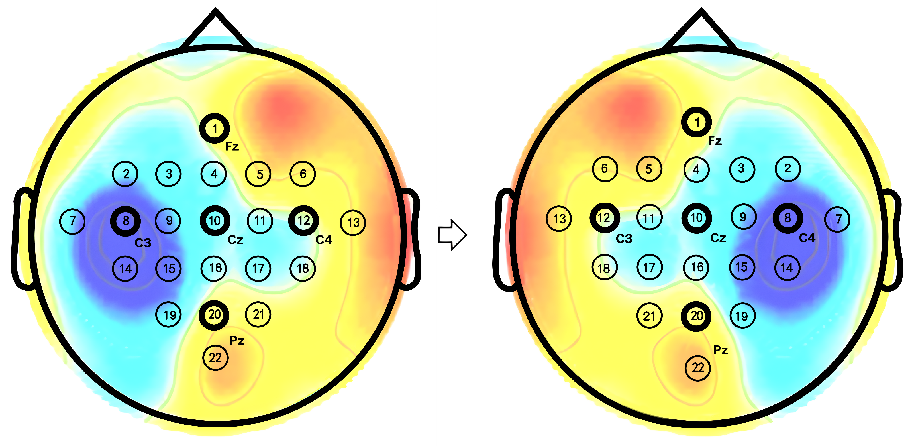
- According to research in the field of neurology, mental imagery of left or right-hand movements induces ERD in the contralateral sensorimotor regions of the brain. Based on this finding, this study introduces mirror contrastive learning (MCL), which enhances the accuracy of identifying the spatial distribution of ERD/ERS by contrasting the original EEG signals with their mirror EEG signals obtained by exchanging the channels of the left and right hemispheres.
- (2)
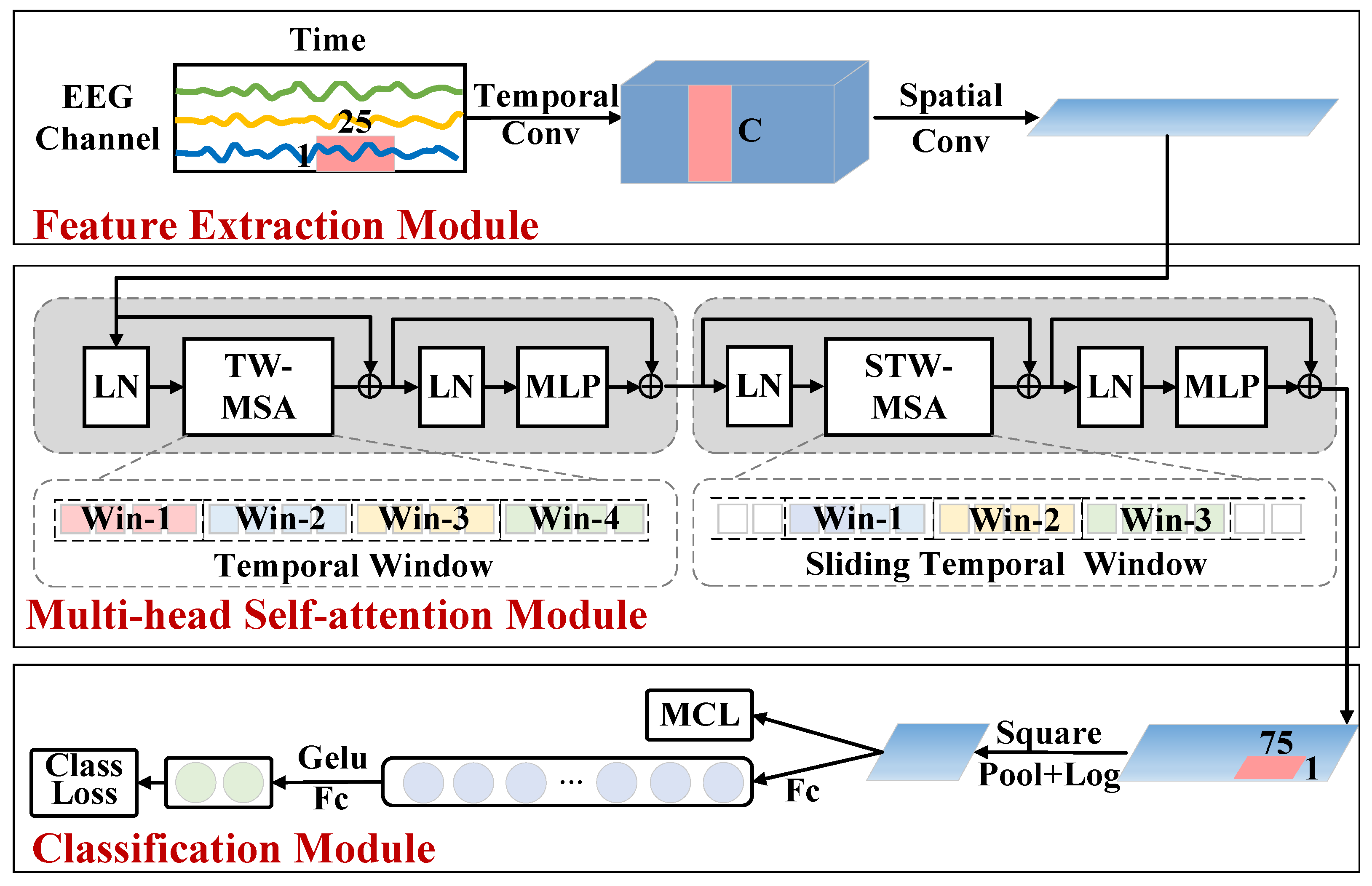
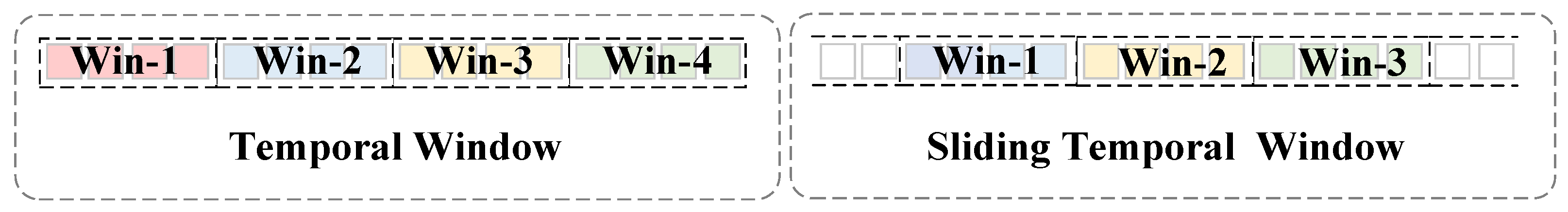
- For subject-independent EEG recognition, a temporal sliding window transformer (SWT) is proposed to achieve high temporal resolution in feature extraction while maintaining manageable computational complexity. Specifically, the self-attention scores are computed within temporal windows, and as these windows slide along the EEG signal’s temporal dimension, the information from different temporal windows can interact with each other.
- (3)
- The experimental results on subject-independent based MI EEG signal recognition demonstrate the effectiveness of MCL-SWT method. Parameter sensitivity experiments demonstrated the robustness of the MCL-SWT model, and feature visualization and ablation studies further validated the effectiveness of the MCL method.
2. Method
2.1. Notations and Definitions
2.2. Sliding Window Transformer Model
2.2.1. Feature Extraction Module
2.2.2. Multi-Head Self-Attention Module
2.2.3. Classification Module
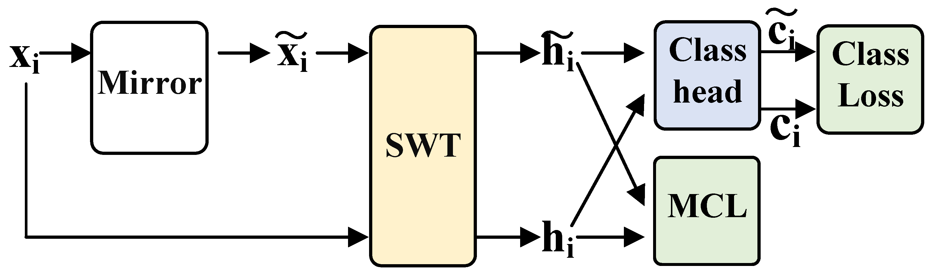
2.3. Mirror Contrastive Learning
2.3.1. Mirror EEG Signal
2.3.2. Mirror Contrastive Loss Function
2.3.3. Model Training Loss
| Algorithm 1 The MCL-SWT Method |
|
3. Experiment and Data
3.1. Data
3.2. Data Preprocessing
3.3. Experiment Settings
4. Results
4.1. Performance Comparison of Subject-Independent MI Recogination
4.2. Sensitivity Analysis of Hyperparameters
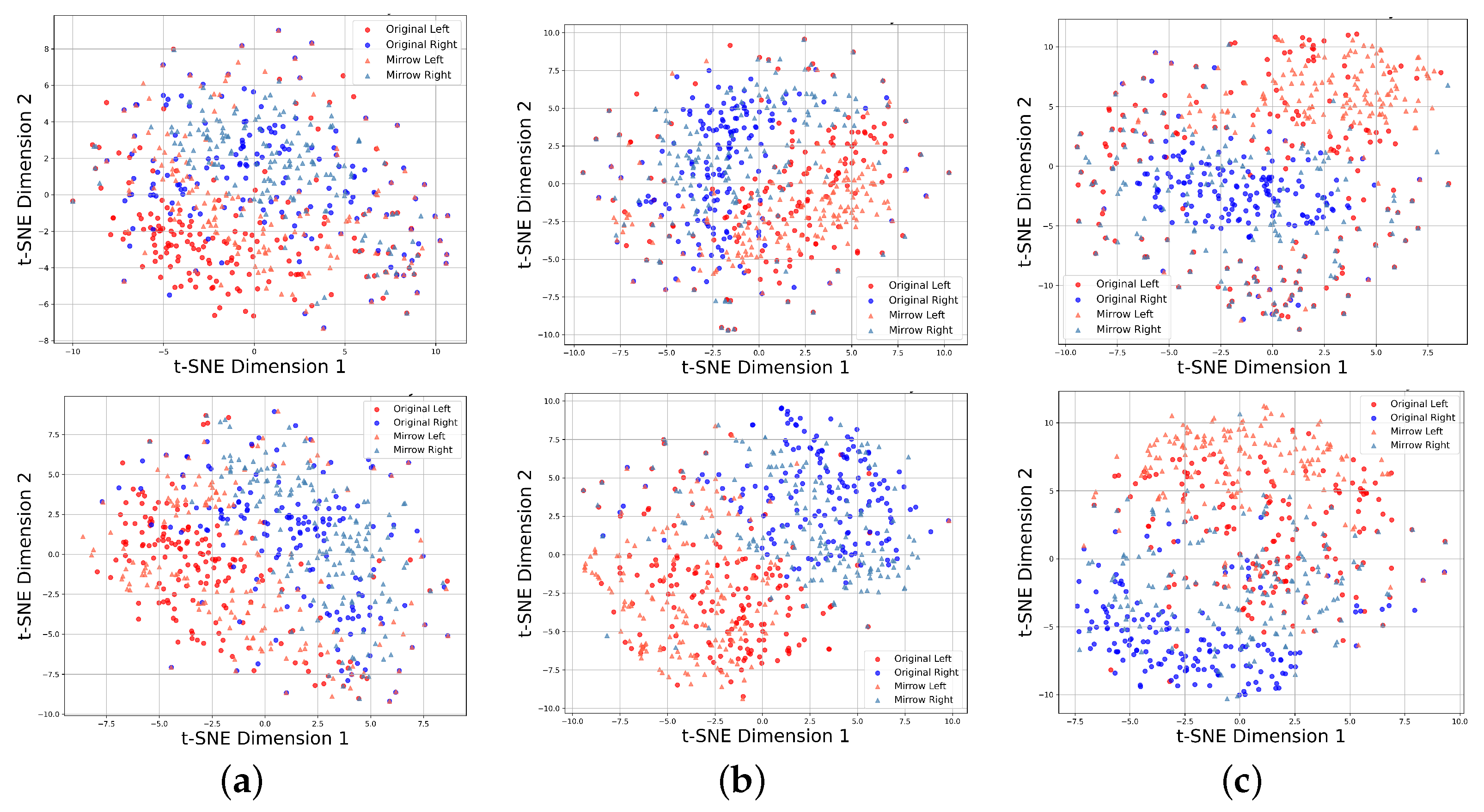
4.3. Feature Visualization
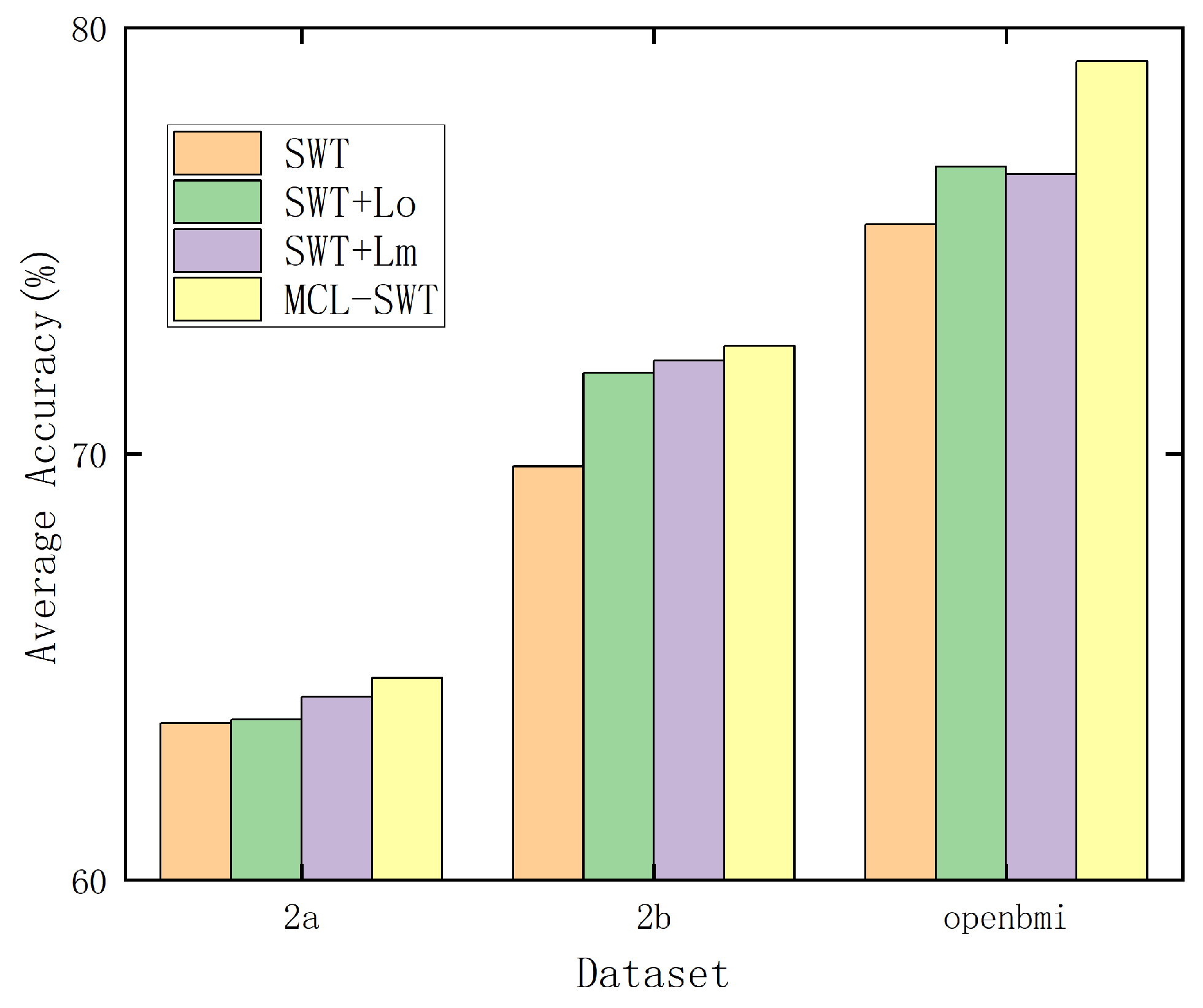
4.4. Ablation Experiment on Mirror Contrastive Loss
4.5. Computing Complexity Analysis
5. Discussion
6. Conclusions
Author Contributions
Funding
Institutional Review Board Statement
Informed Consent Statement
Data Availability Statement
Conflicts of Interest
References
- Wolpaw, J.R. Brain-computer interfaces (BCIs) for communication and control. In Proceedings of the 9th International ACM SIGACCESS Conference on Computers and Accessibility, Tempe, AZ, USA, 15–17 October 2007; pp. 1–2. [Google Scholar]
- Shanechi, M.M. Brain–Machine Interfaces from Motor to Mood. Nat. Neurosci. 2019, 22, 1554–1564. [Google Scholar] [CrossRef]
- Benson, P.J. Decoding brain-computer interfaces. Science 2018, 360, 615–616. [Google Scholar]
- Arpaia, P.; Esposito, A.; Natalizio, A.; Parvis, M. How to successfully classify EEG in motor imagery BCI: A metrological analysis of the state of the art. J. Neural Eng. 2022, 19, 031002. [Google Scholar] [CrossRef] [PubMed]
- Burwell, S.; Sample, M.; Racine, E. Ethical aspects of brain computer interfaces: A scoping review. BMC Med. Ethics 2017, 18, 1–11. [Google Scholar] [CrossRef]
- Altaheri, H.; Muhammad, G.; Alsulaiman, M.; Amin, S.U.; Altuwaijri, G.A.; Abdul, W.; Bencherif, M.A.; Faisal, M. Deep learning techniques for classification of electroencephalogram (EEG) motor imagery (MI) signals: A review. Neural Comput. Appl. 2023, 35, 14681–14722. [Google Scholar] [CrossRef]
- Zhang, S.; Ang, K.K.; Zheng, D.; Hui, Q.; Chen, X.; Li, Y.; Tang, N.; Chew, E.; Lim, R.Y.; Guan, C. Learning eeg representations with weighted convolutional siamese network: A large multi-session post-stroke rehabilitation study. IEEE Trans. Neural Syst. Rehabil. Eng. 2022, 30, 2824–2833. [Google Scholar] [CrossRef]
- Luo, J.; Wang, Y.; Xia, S.; Lu, N.; Ren, X.; Shi, Z.; Hei, X. A shallow mirror transformer for subject-independent motor imagery BCI. Comput. Biol. Med. 2023, 164, 107254. [Google Scholar] [CrossRef]
- Zhu, X.; Meng, M.; Yan, Z.; Luo, Z. Motor Imagery EEG Classification Based on Multi-Domain Feature Rotation and Stacking Ensemble. Brain Sci. 2025, 15, 50. [Google Scholar] [CrossRef]
- Fraiwan, L.; Lweesy, K.; Khasawneh, N.; Wenz, H.; Dickhaus, H. Automated sleep stage identification system based on time–frequency analysis of a single EEG channel and random forest classifier. Comput. Methods Prog. Biomed. 2012, 108, 10–19. [Google Scholar] [CrossRef]
- Bishop, C.M.; Nasrabadi, N.M. Pattern Recognition and Machine Learning; Springer: Berlin/Heidelberg, Germany, 2006; Volume 4. [Google Scholar]
- Lemm, S.; Blankertz, B.; Curio, G.; Muller, K.R. Spatio-spectral filters for improving the classification of single trial EEG. IEEE Trans. Biomed. Eng. 2005, 52, 1541–1548. [Google Scholar] [CrossRef]
- Ang, K.K.; Chin, Z.Y.; Zhang, H.; Guan, C. Filter bank common spatial pattern (FBCSP) in brain-computer interface. In Proceedings of the 2008 IEEE International Joint Conference on Neural Networks (IEEE World Congress on Computational Intelligence), Hong Kong, China, 1–8 June 2008; IEEE: Piscataway, NJ, USA, 2008; pp. 2390–2397. [Google Scholar]
- Gu, H.; Chen, T.; Ma, X.; Zhang, M.; Sun, Y.; Zhao, J. CLTNet: A Hybrid Deep Learning Model for Motor Imagery Classification. Brain Sci. 2025, 15, 124. [Google Scholar] [CrossRef] [PubMed]
- Bouchane, M.; Guo, W.; Yang, S. Hybrid CNN-GRU Models for Improved EEG Motor Imagery Classification. Sensors 2025, 25, 1399. [Google Scholar] [CrossRef] [PubMed]
- Schirrmeister, R.T.; Springenberg, J.T.; Fiederer, L.D.J.; Glasstetter, M.; Eggensperger, K.; Tangermann, M.; Hutter, F.; Burgard, W.; Ball, T. Deep learning with convolutional neural networks for EEG decoding and visualization. Hum. Brain Mapp. 2017, 38, 5391–5420. [Google Scholar] [CrossRef] [PubMed]
- Jiao, Y.; Zhang, Y.; Chen, X.; Yin, E.; Jin, J.; Wang, X.; Cichocki, A. Sparse group representation model for motor imagery EEG classification. IEEE J. Biomed. Health Inform. 2018, 23, 631–641. [Google Scholar] [CrossRef]
- Autthasan, P.; Chaisaen, R.; Sudhawiyangkul, T.; Rangpong, P.; Kiatthaveephong, S.; Dilokthanakul, N.; Bhakdisongkhram, G.; Phan, H.; Guan, C.; Wilaiprasitporn, T. MIN2Net: End-to-end multi-task learning for subject-independent motor imagery EEG classification. IEEE Trans. Biomed. Eng. 2021, 69, 2105–2118. [Google Scholar] [CrossRef]
- Pfurtscheller, G.; Da Silva, F.L. Event-related EEG/MEG synchronization and desynchronization: Basic principles. Clin. Neurophysiol. 1999, 110, 1842–1857. [Google Scholar] [CrossRef]
- Makeig, S.; Bell, A.; Jung, T.P.; Sejnowski, T.J. Independent component analysis of electroencephalographic data. Adv. Neural Inf. Process. Syst. 1995, 8, 145–151. [Google Scholar]
- Kim, H.; Yoshimura, N.; Koike, Y. Characteristics of kinematic parameters in decoding intended reaching movements using electroencephalography (EEG). Front. Neurosci. 2019, 13, 1148. [Google Scholar] [CrossRef]
- Zhao, H.; Zheng, Q.; Ma, K.; Li, H.; Zheng, Y. Deep representation-based domain adaptation for nonstationary EEG classification. IEEE Trans. Neural Netw. Learn. Syst. 2020, 32, 535–545. [Google Scholar] [CrossRef]
- Xu, L.; Xu, M.; Ke, Y.; An, X.; Liu, S.; Ming, D. Cross-dataset variability problem in EEG decoding with deep learning. Front. Hum. Neurosci. 2020, 14, 103. [Google Scholar] [CrossRef]
- Rodrigues, P.L.C.; Jutten, C.; Congedo, M. Riemannian procrustes analysis: Transfer learning for brain–computer interfaces. IEEE Trans. Biomed. Eng. 2018, 66, 2390–2401. [Google Scholar] [CrossRef] [PubMed]
- Zhang, K.; Robinson, N.; Lee, S.W.; Guan, C. Adaptive transfer learning for EEG motor imagery classification with deep convolutional neural network. Neural Netw. 2021, 136, 1–10. [Google Scholar] [CrossRef] [PubMed]
- Jia, Z.; Lin, Y.; Wang, J.; Yang, K.; Liu, T.; Zhang, X. MMCNN: A Multi-branch Multi-scale Convolutional Neural Network for Motor Imagery Classification. In Machine Learning and Knowledge Discovery in Databases; Hutter, F., Kersting, K., Lijffijt, J., Valera, I., Eds.; Springer: Cham, Switzerland, 2021; pp. 736–751. [Google Scholar]
- Liu, Z.; Lin, Y.; Cao, Y.; Hu, H.; Wei, Y.; Zhang, Z.; Lin, S.; Guo, B. Swin transformer: Hierarchical vision transformer using shifted windows. In Proceedings of the IEEE/CVF International Conference on Computer Vision, Montreal, BC, Canada, 11–17 October 2021; pp. 10012–10022. [Google Scholar]
- Altaheri, H.; Muhammad, G.; Alsulaiman, M. Physics-informed attention temporal convolutional network for EEG-based motor imagery classification. IEEE Trans. Ind. Inform. 2022, 19, 2249–2258. [Google Scholar] [CrossRef]
- Luo, J.; Mao, Q.; Shi, W.; Shi, Z.; Wang, X.; Lu, X.; Hei, X. Mirror contrastive loss based sliding window transformer for subject-independent motor imagery based EEG signal recognition. In Proceedings of the Human Brain and Artificial Intelligence, 4th International Workshop, HBAI 2024, held in Conjunction with IJCAI 2024, Jeju Island, Republic of Korea, 3 August 2024. [Google Scholar]
- Ioffe, S.; Szegedy, C. Batch normalization: Accelerating deep network training by reducing internal covariate shift. In Proceedings of the International Conference on Machine Learning, Lille, France, 7–9 July 2015; PMLR: Breckenridge, CO, USA, 2015; pp. 448–456. [Google Scholar]
- Ba, J.L.; Kiros, J.R.; Hinton, G.E. Layer normalization. arXiv 2016, arXiv:1607.06450. [Google Scholar]
- Hendrycks, D.; Gimpel, K. Gaussian error linear units (gelus). arXiv 2016, arXiv:1606.08415. [Google Scholar]
- Luo, J.; Shi, W.; Lu, N.; Wang, J.; Chen, H.; Wang, Y.; Lu, X.; Wang, X.; Hei, X. Improving the performance of multisubject motor imagery-based BCIs using twin cascaded softmax CNNs. J. Neural Eng. 2021, 18, 036024. [Google Scholar] [CrossRef]
- Hadsell, R.; Chopra, S.; LeCun, Y. Dimensionality reduction by learning an invariant mapping. In Proceedings of the 2006 IEEE Computer Society Conference on Computer Vision And Pattern Recognition (CVPR’06), New York, NY, USA, 17–22 June 2006; IEEE: Piscataway, NJ, USA, 2006; Volume 2, pp. 1735–1742. [Google Scholar]
- Tangermann, M.; Müller, K.R.; Aertsen, A.; Birbaumer, N.; Braun, C.; Brunner, C.; Leeb, R.; Mehring, C.; Miller, K.J.; Müller-Putz, G.R.; et al. Review of the BCI competition IV. Front. Neurosci. 2012, 6, 55. [Google Scholar]
- Lee, M.H.; Kwon, O.Y.; Kim, Y.J.; Kim, H.K.; Lee, Y.E.; Williamson, J.; Fazli, S.; Lee, S.W. EEG dataset and OpenBMI toolbox for three BCI paradigms: An investigation into BCI illiteracy. GigaScience 2019, 8, giz002. [Google Scholar] [CrossRef]
- Kingma, D.P.; Ba, J. Adam: A method for stochastic optimization. arXiv 2014, arXiv:1412.6980. [Google Scholar]
- Lawhern, V.J.; Solon, A.J.; Waytowich, N.R.; Gordon, S.M.; Hung, C.P.; Lance, B.J. EEGNet: A compact convolutional neural network for EEG-based brain–computer interfaces. J. Neural Eng. 2018, 15, 056013. [Google Scholar] [CrossRef]
- Mane, R.; Chew, E.; Chua, K.; Ang, K.K.; Robinson, N.; Vinod, A.P.; Lee, S.W.; Guan, C. FBCNet: A multi-view convolutional neural network for brain-computer interface. arXiv 2021, arXiv:2104.01233. [Google Scholar]
- Van der Maaten, L.; Hinton, G. Visualizing data using t-SNE. J. Mach. Learn. Res. 2008, 9, 2579–2605. [Google Scholar]


| 2a-0 Hz | 2a-4 Hz | 2b-0 Hz | 2b-4 Hz | ||
|---|---|---|---|---|---|
| Avg Acc/ Kappa | Shallow | 63.72/0.29 | 60.76/0.25 | 72.70/0.46 | 67.06/0.34 |
| Deep | 60.55/0.25 | 60.80/0.25 | 71.55/0.44 | 65.93/0.32 | |
| EEGNet | 60.58/0.25 | 59.52/0.23 | 71.21/0.44 | 65.91/0.32 | |
| FBCNet | 60.56/0.25 | 59.73/0.23 | 70.55/0.43 | 65.29/0.31 | |
| ATCNet | 58.87/0.22 | 57.45/0.20 | 68.47/0.36 | 64.69/0.30 | |
| SWT | 66.00/0.33 | 63.68/0.28 | 74.50/0.49 | 69.71/0.40 | |
| MCL-SWT | 66.56/0.33 | 64.74/0.30 | 75.85/0.52 | 72.54/0.45 | |
| Acc/ Kappa | Shallow | 63.66/0.28 | 61.18/0.26 | 73.45/0.47 | 68.70/0.36 |
| Deep | 61.27/0.26 | 61.34/0.26 | 72.89/0.46 | 66.51/0.34 | |
| EEGNet | 61.19/0.26 | 58.72/0.22 | 72.24/0.45 | 66.20/0.33 | |
| FBCNet | 60.86/0.25 | 58.36/0.22 | 71.18/0.44 | 65.53/0.31 | |
| ATCNet | 59.34/0.23 | 57.78/0.20 | 69.13/0.39 | 63.78/0.27 | |
| SWT | 66.13/0.33 | 63.58/0.28 | 74.58/0.49 | 69.79/0.40 | |
| MCL-SWT | 66.48/0.33 | 64.52/0.30 | 75.62/0.51 | 73.27/0.47 | |
| Max Acc/ Kappa | Shallow | 67.28/0.34 | 65.36/0.32 | 75.18/0.51 | 71.69/0.45 |
| Deep | 66.05/0.33 | 65.35/0.32 | 73.73/0.48 | 71.68/0.45 | |
| EEGNet | 65.51/0.32 | 64.51/0.30 | 73.31/0.47 | 71.16/0.44 | |
| FBCNet | 66.46/0.33 | 63.89/0.29 | 72.93/0.46 | 70.98/0.43 | |
| ATCNet | 64.11/0.29 | 62.18/0.28 | 70.84/0.43 | 68.22/0.36 | |
| SWT | 66.82/0.34 | 64.81/0.30 | 75.49/0.51 | 74.12/0.48 | |
| MCL-SWT | 67.37/0.35 | 65.49/0.31 | 76.37/0.53 | 75.49/0.51 |
| Shallow | Deep | EEGNet | FBCNet | ATCNet | MCL-SWT | ||
|---|---|---|---|---|---|---|---|
| Avg Acc/ Kappa | Fold1 | 81.61/0.63 | 79.56/0.59 | 80.17/0.60 | 79.00/0.58 | 80.89/0.62 | 82.56/0.65 |
| Fold2 | 77.67/0.55 | 75.89/0.52 | 75.94/0.52 | 71.56/0.43 | 73.72/0.47 | 80.01/0.60 | |
| Fold3 | 78.33/0.57 | 80.44/0.61 | 82.00/0.64 | 82.39/0.65 | 83.83/0.68 | 76.38/0.53 | |
| Fold4 | 81.00/0.62 | 81.22/0.62 | 82.06/0.64 | 79.11/0.58 | 80.06/0.60 | 85.51/0.71 | |
| Fold5 | 74.39/0.49 | 72.28/0.45 | 76.89/0.54 | 71.67/0.43 | 72.94/0.46 | 75.48/0.51 | |
| Fold6 | 80.33/0.61 | 82.61/0.65 | 82.75/0.66 | 76.89/0.54 | 81.78/0.64 | 80.46/0.61 | |
| Fold7 | 70.33/0.41 | 69.22/0.38 | 70.44/0.41 | 67.83/0.36 | 72.28/0.45 | 74.05/0.48 | |
| Avg | 77.67/0.55 | 77.32/0.55 | 78.61/0.57 | 75.49/0.51 | 77.93/0.56 | 79.21/0.58 |
| MCL-SWT vs. | Shallow | Deep | EEGNet | FBCNet | ATCNet |
|---|---|---|---|---|---|
| p-Values | 0.0036 | 0.0020 | 0.0005 | 0.0007 | 0.0001 |
| 4 Heads | 8 Heads | 10 Heads | |
|---|---|---|---|
| 1 block | 74.71/0.49 | 74.50/0.49 | 74.73/0.49 |
| 2 block | 74.30/0.48 | 74.20/0.48 | 74.45/0.49 |
| 3 block | 73.16/0.46 | 73.67/0.47 | 73.26/0.46 |
| hyperparameter values | |||
| Average Accuracy | 72.54 | 72.29 | 72.26 |
| hyperparameter values | |||
| Average Accuracy | 71.95 | 72.54 | 72.02 |
| SWT | sub1 | sub2 | sub3 | sub4 | sub5 | sub6 | sub7 | sub8 | sub9 | Avg | ||
|---|---|---|---|---|---|---|---|---|---|---|---|---|
| ✓ | 66.53 | 54.39 | 88.65 | 58.92 | 53.87 | 57.51 | 62.35 | 71.52 | 59.39 | 63.68 | ||
| ✓ | ✓ | 66.72 | 58.73 | 88.77 | 58.01 | 54.31 | 56.82 | 60.34 | 74.03 | 56.19 | 63.77 | |
| ✓ | ✓ | 67.76 | 58.33 | 89.97 | 57.89 | 55.37 | 58.51 | 61.58 | 72.33 | 56.97 | 64.30 | |
| ✓ | ✓ | ✓ | 68.81 | 57.26 | 89.83 | 59.67 | 56.95 | 59.85 | 59.18 | 73.18 | 57.94 | 64.74 |
| SWT | sub1 | sub2 | sub3 | sub4 | sub5 | sub6 | sub7 | sub8 | sub9 | Avg | ||
|---|---|---|---|---|---|---|---|---|---|---|---|---|
| ✓ | 65.83 | 53.12 | 54.75 | 80.23 | 73.74 | 67.60 | 73.30 | 83.50 | 75.32 | 69.71 | ||
| ✓ | ✓ | 69.61 | 54.15 | 55.50 | 81.63 | 78.71 | 68.70 | 75.70 | 86.23 | 76.85 | 71.90 | |
| ✓ | ✓ | 68.36 | 53.97 | 56.76 | 82.82 | 78.84 | 70.53 | 73.76 | 85.54 | 79.09 | 72.19 | |
| ✓ | ✓ | ✓ | 69.50 | 55.69 | 57.13 | 82.71 | 78.17 | 69.86 | 74.75 | 86.93 | 78.13 | 72.54 |
| SWT | Fold1 | Fold2 | Fold3 | Fold4 | Fold5 | Fold6 | Fold7 | Avg | ||
|---|---|---|---|---|---|---|---|---|---|---|
| ✓ | 78.00 | 75.61 | 74.71 | 76.43 | 73.31 | 78.11 | 71.56 | 75.39 | ||
| ✓ | ✓ | 80.93 | 76.90 | 75.66 | 78.05 | 74.02 | 79.31 | 72.38 | 76.75 | |
| ✓ | ✓ | 80.68 | 77.74 | 75.61 | 77.98 | 74.25 | 78.28 | 71.35 | 76.56 | |
| ✓ | ✓ | ✓ | 82.56 | 80.01 | 76.38 | 85.51 | 75.48 | 80.46 | 74.05 | 79.21 |
| Shallow | Deep | EEGNet | FBCNet | ATCNet | MCL-SWT | |
|---|---|---|---|---|---|---|
| Para num (M) | 10 | 268 | 3 | 3 | 37 | 155 |
| Infer time (ms) | 0.56 | 1.42 | 2.48 | 37.64 | 15.37 | 8.36 |
Disclaimer/Publisher’s Note: The statements, opinions and data contained in all publications are solely those of the individual author(s) and contributor(s) and not of MDPI and/or the editor(s). MDPI and/or the editor(s) disclaim responsibility for any injury to people or property resulting from any ideas, methods, instructions or products referred to in the content. |
© 2025 by the authors. Licensee MDPI, Basel, Switzerland. This article is an open access article distributed under the terms and conditions of the Creative Commons Attribution (CC BY) license (https://creativecommons.org/licenses/by/4.0/).
Share and Cite
Mao , Q.; Zhu , H.; Yan , W.; Zhao , Y.; Hei , X.; Luo , J. MCL-SWT: Mirror Contrastive Learning with Sliding Window Transformer for Subject-Independent EEG Recognition. Brain Sci. 2025, 15, 460. https://doi.org/10.3390/brainsci15050460
Mao Q, Zhu H, Yan W, Zhao Y, Hei X, Luo J. MCL-SWT: Mirror Contrastive Learning with Sliding Window Transformer for Subject-Independent EEG Recognition. Brain Sciences. 2025; 15(5):460. https://doi.org/10.3390/brainsci15050460
Chicago/Turabian StyleMao , Qi, Hongke Zhu , Wenyao Yan , Yu Zhao , Xinhong Hei , and Jing Luo . 2025. "MCL-SWT: Mirror Contrastive Learning with Sliding Window Transformer for Subject-Independent EEG Recognition" Brain Sciences 15, no. 5: 460. https://doi.org/10.3390/brainsci15050460
APA StyleMao , Q., Zhu , H., Yan , W., Zhao , Y., Hei , X., & Luo , J. (2025). MCL-SWT: Mirror Contrastive Learning with Sliding Window Transformer for Subject-Independent EEG Recognition. Brain Sciences, 15(5), 460. https://doi.org/10.3390/brainsci15050460