Abstract
In Indonesia, there is a need to improve the efficiency of damage assessments of the agricultural insurance system for paddy rice producers affected by floods, droughts, pests, and diseases. In this study, we develop a method to estimate the transplanting date required for damage assessments of paddy rice fields. The study area is the Cihea irrigation district in West Java, Republic of Indonesia. Backscattering coefficients of VH polarization measured by a synthetic aperture radar onboard the Sentinel-1 satellite were used for the estimations. We investigated the accuracy of the estimations of the proposed method by smoothing out the time-series data, applying a speckle filter, and by signal synthesis of the surrounding fields. It was found that these variations effectively improved the estimation accuracy. To further improve the estimation accuracy, the data for all incident angles were used after correcting the incident angle dependence of the backscattering coefficients for three types of data with different incident angles (32°, 41°, and 45°) obtained in the study area. The estimated transplanting date for each field in the test site was compared with the transplanting date obtained through interviews. The standard deviations of the estimation errors for the four cropping periods from March 2018 to February 2020 were found to be ~5–6 days, and the percentages of estimation errors in transplanting dates within 5, 10, and 15 days were estimated to be 69%, 92%, and 97%, respectively. It was confirmed that a sufficiently reliable transplanting date estimation can be obtained ~10–15 days after transplantation.
1. Introduction
According to the United Nations’ world population estimate, the global population is expected to reach 9.7 billion by 2050 [1], and the global demand for grains is increasing every year, in combination with particularly pronounced economic growth in developing countries [2]. Furthermore, there have been grave concerns regarding global warming and consequent climate change characterized by an increase in natural disasters such as floods and droughts, which can adversely affect agricultural production [3]. Therefore, agricultural insurance is attracting attention as one of the measures to stabilize food supplies by helping farmers affected by such disasters. In Indonesia, the world’s third-largest rice producer, an agricultural insurance system is in place to help rice producers affected by floods, droughts, pests, and diseases [4,5,6,7]. The system determines insurance payouts based on the results of damage assessments in the field where damage has occurred. At present, damage assessments are performed by damage evaluators from the state government (pest observer) and the insurance company (loss adjuster). However, the area covered by each pest observer in the field survey is very large, and the evaluation of the entire target area is very time-consuming. Furthermore, in Indonesia, the rugged terrain and limited roads make it difficult to assess damage, because access to paddy fields is sometimes limited [8]. To evaluate damage to rice paddy fields, it is important to determine the transplanting date for the following reasons. First, the insurance coverage period is set from the transplanting of paddy rice to the harvesting period; hence, it is necessary to determine the transplanting date to set the insurance start date. Second, to evaluate the flood damage, it is required that the growth stage of the rice plants during the flood should be 30 days or later from the transplanting date. Therefore, it is necessary to know the transplanting date to determine the target fields for further investigations. However, at present, the only way to determine the transplanting date is by checking the records of the farmer or the agricultural organization; therefore, a more objective and scientific method is required to determine the transplanting date for damage assessments. A new method should be developed for estimating the transplanting date using remote sensing technology that is fast, accurate, and low cost.
Satellite observation is suitable for efficiently investigating vast paddy field areas. It has been reported that the transplanting date of rice can be estimated by the time-series data of vegetation indices, such as normalized difference vegetation index (NDVI) and enhanced vegetation index, obtained from the reflectance measured by optical satellites [9,10]. However, visible-to-near-infrared sunlight is often blocked by clouds, and the ground surface may not be clearly observed by optical satellites. In contrast, microwaves with wavelengths of several centimeters to several tens of centimeters, such as X band (~3–4 cm), C band (~4–8 cm), and L band (~20–60 cm), are transmitted through clouds but scattered by vegetation. Therefore, synthetic aperture radar (SAR), which can observe the scattering of such microwaves, can be used to observe the ground surface even in areas covered with clouds. Crop monitoring using SAR has a long history [11], and several studies on paddy field classification using the SAR satellite data, such as RADARSAT-2, TerraSAR-X, and Sentinel-1, have been conducted [12,13,14,15]. In Indonesia, studies using SAR for the extraction of flood areas [16], crop classification in upland fields [17], growth stage classification of paddy rice [18], development of growth model for paddy rice [19], and so on have been conducted. In a study on transplanting date estimation using the SAR, the flooding/transplanting date was estimated with an accuracy of nine days by obtaining the time when the time-series data of the X-band backscattering coefficient (BSC) obtained by TerraSAR-X fell below the value threshold assumed to represent the transplanting date [20]. In the case of our study area, however, it is difficult to set a uniform threshold of BSC because it is not always flooded at the time of transplanting, and the signal intensity of the SAR backscattering data varies with field conditions. In addition, the TerraSAR-X data used by Asilo et al. was at 11-day intervals; however, it is expected that a more accurate transplanting date estimation is possible by using the data that are more frequently acquired by Sentinel-1. Nguyen et al. [21,22] used the time-series data of the BSC of Sentinel-1 to estimate the start time of rice growth; however, their main purpose was to extract paddy field areas, and the accuracy in estimating the transplanting date was not mentioned. The purpose of this study is to develop a new method, which is quick, accurate, and low cost, for estimating the transplanting date required for damage assessments of rice paddy fields in Indonesia. Moreover, we examined how to accurately derive the transplanting date from the C-band SAR data of Sentinel-1.
2. Materials and Methods
2.1. Study Area
The study area is the Cihea irrigation district in the north-eastern part of Cianjur Province, West Java, Indonesia. Figure 1 shows a map of the Cihea irrigation district (the area surrounded by a dashed line in Figure 1b); the area is sandwiched between two rivers flowing northward—the Cisokon and Citarum rivers. The size of this area is approximately 12 km from east to west and 15 km from north to south. A training center of the West Java Province Agricultural Administration is located near the center of the Cihea irrigation district (6°50′42″ South, 107°16′15″ East), and the 250 ha area near the training center (the area surrounded by the solid line in Figure 1b) was used as the test site for the analysis. The study area is located in the tropics, which has a dry season from April to October and a wet/rainy season from November to March. Here, rice is planted twice (once in the dry season and once in the rainy season) or three times a year (twice in the dry season and once in the rainy season). Furthermore, since the irrigation water is derived from rivers and is therefore affected by the rainfall, the transplanting date varies depending on the cropping season and field. The field is not always in a flooded state at the time of transplanting, and the signal intensity of the SAR data also varies. Furthermore, many fields have small areas; therefore, high spatial resolution is required for analysis. The transplanting date estimation method must take into consideration the characteristics of the study area.
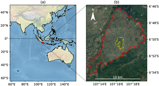
Figure 1.
Maps showing the study area as well as the area around it. (a) Around Java Island. The Cihea irrigation district is located in the circle. (b) Around the Cihea irrigation district. The dashed line indicates the boundary of the Cihea irrigation district and the solid line indicates the boundary of the test site.
2.2. Methodology
2.2.1. Overview
The BSC obtained from the SAR data decreases as the ground surface of the study area becomes smoother, and it is considered to take the minimum value around the transplanting date in the paddy fields. The Sentinel-1 data include VV and VH polarizations; however, our preliminary investigation showed that the BSC of the VV polarization decreases significantly, even outside the transplanting period. Therefore, only VH polarization was used in the analysis. Owing to the characteristics of the SAR amplitude image, random noise (speckle noise) that differs from pixel to pixel is unavoidable; therefore, the local minima of the BSC time-series data were searched after the application of an appropriate noise reduction technique. The upper limit of the BSC was determined to exclude signals other than the transplanting period, and a local minimum at which the differential signal intensity between the minimum and the upper limit values becomes the maximum was found in order to obtain a transplanting date estimation value for each pixel. For a paddy field, wherein the pixels of the field in the image are known, the transplanting date estimation was obtained through the weighted average of transplanting date estimates of each pixel within the field, as this provides a more accurate date.
In the transplanting date estimation, two kinds of estimations are provided, namely, preliminary and final estimations. Preliminary estimation is updated as new Sentinel-1 data become available, and is used for quick evaluations when damage occurs to the paddy field. If the transplanting date is close to the date of the latest data acquisition, the preliminary estimation may contain errors; thus, final estimation is carried out after the transplanting period for each cropping season and used for verification of preliminary estimation (see Section 2.2.4 for details). The accuracy of the preliminary estimation increases with the accumulation of new satellite data, and eventually, an estimation close to the final estimation is obtained. The details are described below.
2.2.2. Data Used
Sentinel-1 is an Earth observation satellite constellation equipped with a C-band SAR operated by the European Space Agency, and two Sentinel-1 satellites, i.e., Sentinel-1A and Sentinel-1B were launched on 3 April 2014 and 25 April 2016, respectively. The Sentinel-1 satellite data are provided free of cost through the Copernicus Open Access Hub, and Sentinel-1A Level-1 Ground Range Detected data (IW mode, High resolution, dual VV + VH polarization) are used to estimate the transplanting date. For the data in the range and azimuth directions, the look numbers are 5 and 1, respectively, and the spatial resolutions are 20 m and 22 m, respectively. The sampling interval is 10 m in both directions. The repeat cycle of Sentinel-1A is 12 days; however, due to the overlapping effect, three types of data with incident angles 32° (descending), 41° (ascending), and 45° (descending) can be obtained at intervals of 4–5 days when combining ascending and descending.
2.2.3. Preprocessing
The BSC of the VH polarization is calculated by preprocessing the Sentinel-1 data, including the study area, using the Python interface (snappy) of the Sentinels Application Platform (SNAP) in the following order.
- Orbit file: Obtain an accurate orbit state vector of the satellite.
- Subset: Clip the region of interest (East longitude 107.201–107.367°, South latitude 6.760–6.910°).
- Calibration: Convert digital value to BSC, σ0, where the area normalization is aligned with ground range plane; or β0, where the area normalization is aligned with the slant range.
- Terrain flattening: Convert β0 to γ0 (where the area normalization is aligned with a plane perpendicular to a slant range).
- Speckle filter: Apply a speckle filter (default: Lee filter with a size of 3 × 3).
- Terrain correction: Perform geometric correction using a digital elevation model (SRTM 3Sec) and interpolate on a Universal Transverse Mercator (UTM) grid at 10 m intervals including reference points (N 9,236,000 m, E 743,800 m) by bilinear interpolation.
- Logarithmic conversion: Convert BSC to a decibel value.
After these preprocesses, the extents of the UTM common grid (E 743,800–757,310 m, N 9,235,810–9,251,810 m) are clipped and saved in the GeoTIFF format.
2.2.4. Signal Search
The BSC time-series data are generated from the GeoTIFF files of the Sentinel-1 data acquired during the period that includes a sufficient margin for the transplanting date search period. In cases of preliminary estimation, the end of the transplanting date search period was set to the date of the latest data acquisition, and the length of the transplanting date search period was determined such that the estimation was not affected by the previous transplantation or the latest flood. For the study area, transplant to harvest requires a period of approximately 90–100 days; therefore, the length of the transplanting date search period was set to 60 days. (For example, if the latest data was obtained on 1 April 2019, the transplanting date search period would be 31 January 2019–1 April 2019.) In the case of the final estimation, the transplanting date search period was determined as a period covering the transplanting period of all target fields (for example, 15 March 2019–15 June 2019 for the first crop at the test site in the dry season of 2019). When reading the data, as the BSC is dependent on the incident angle, the difference between the three types of data (incident angles of 32°, 41°, and 45°) was reduced by subtracting the offset of the data with incident angles of 41° and 45° relative to the data with the incident angle of 32°. This offset was estimated from the average of the time-series data for each pixel over three years. Further, to reduce noise, the time-series data for each pixel was smoothed out by a cubic smoothing spline [23], and the interpolated values were obtained on a time grid with an interval of 0.1 days. With this interpolation, the time-series data are represented by a smooth spline curve that does not necessarily pass through the data points. The smoothness of the spline curve can be adjusted by the smoothing out parameter psm (default: 0.01. A perfectly smoothed out straight line is obtained with psm = 0, and a cubic spline curve through all the data points without smoothing out is obtained with psm = 1). From the smoothed out data obtained with this approach, all the local minima within the transplanting date search period were determined. In a preliminary estimation, when the value of the BSC decreased near the end of the time-series data (i.e., the date of the latest data), the end point was added as a local minimum. Then, the date tij and the BSC value vij of each local minimum were obtained (i, j are indices of pixels and local minima, respectively). Here, the average value for a certain period (default: tij − 20 days to tij + 20 days) centered on the local minima was defined as the BSC value, such that the local minima with small nearby BSCs for a certain long period was given priority. However, for the end points added when performing the preliminary estimation, the end point value itself was used as the BSC value without averaging so that the latest transplanting date was given priority. If the BSC value of the local minimum exceeded the predetermined upper limit vth (default: −13 dB), it was assumed that the obtained signal could not be attributed to the transplanting date, and the corresponding local minimum was excluded. The number Ni of the remaining local minima may be greater than 1, depending on the pixel. The differential signal intensity yij on the transplanting date was defined as follows:
By definition, the differential signal intensity increases as the BSC around the transplanting date decreases.
2.2.5. Signal Synthesis
In most cases in the study area, transplantation was performed on similar days in the vicinity. Subsequently, to obtain a more plausible transplanting date estimate considering the surrounding condition, the differential signal intensities obtained for 120 pixels (i = 1–120) within a radius of approximately 65 m from the target pixel (i = 0) were added, along with Gaussian weights, and the synthesized signal intensity y0 around the target pixel was obtained as follows:
where li is the center-to-center distance between the target pixel 0 and the peripheral pixel i, and σt (six days) and σl (default: 30 m) are the spread width of Gaussian in the time and space directions, respectively. The spread width in the time direction was determined to have an appropriate spread of the synthesized signal in consideration of the estimation error of the transplanting date. With these reasonable spread widths, many Gaussians overlap near the plausible transplanting date.
2.2.6. Pixel-by-Pixel Transplanting Date Estimation
In the study area, the condition at the time of transplantation—flooded or not flooded—varies from field to field; hence, it is difficult to set a uniform threshold of the synthesized signal intensity. Therefore, the day on which the synthesized signal intensity y0 obtained in the transplanting date search period becomes maximum was determined as the transplanting date estimation value for each pixel.
2.2.7. Field-by-Field Transplanting Date Estimation
For the 250 ha test site inside the study area, a shapefile (parcel data) was prepared by extracting the outline of each paddy field and surrounding it with a polygon. The number of fields in the parcel data is 5968, and the average area of each field is 400 m2. For these fields, the transplanting date of a field was estimated by averaging the estimated transplanting dates of the pixels included partially or fully in the polygon surrounding the field. In calculating the average, the synthesized signal intensity of each pixel was used as the default weight.
In the following discussion, unless stated otherwise, “signal” indicates a raw value or a smoothed out value of the BSC. To avoid confusion, the difference between the BSC upper limit and the BSC at the local minimum is called a “differential” signal, and the composite of the differential signals of peripheral pixels is called a “synthesized” signal. Moreover, the average value of the synthesized signals of the pixels inside a field is called a “field average” signal.
2.2.8. Optimization of Transplanting Date Estimation Method
The 250 ha test site was divided into 25 irrigation blocks, each block containing ~100–400 fields. For each block, interviews were conducted to determine the transplanting dates. Table 1 and Figure 2 show the transplanting date (block value) of each block for the first crop in the dry season of 2019 obtained by the interview survey. A block value is a representative value of each block, and actual transplanting dates may have varied within the block; however, differences among blocks were usually within three days. Therefore, the block value is regarded as a true value, and the transplanting date estimation method was optimized such that the estimated value was as close to the block value as possible.

Table 1.
Block values of transplanting date at the test site (first crop in the dry season of 2019). Dates are in YYYY/MM/DD format.
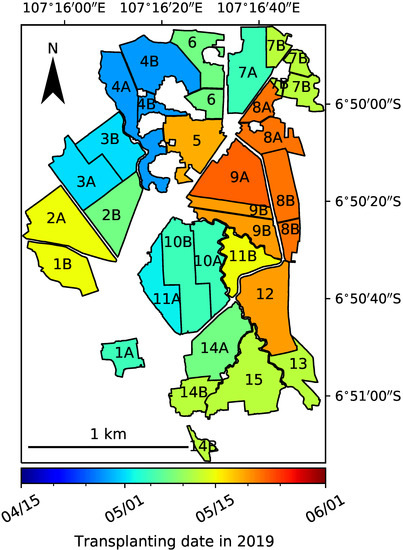
Figure 2.
Map of transplanting date block values at the test site (first crop in the dry season of 2019). The 250ha test site is divided into 25 irrigation blocks, which are color-coded by the transplanting date (block value) obtained from the interview survey for each block.
The transplanting date was estimated for each field in the test site under the default settings listed in Table 2. In the optimization process, the settings (1–18; Table 3) were changed one by one, and the results were compared with those for the default settings. Then, the average (AVG) and standard deviation (STD) of the transplanting date estimation errors (i.e., estimated values minus block values) were calculated. The value of AVG is stable if the setting is fixed and can be corrected by subtracting it from the estimated transplanting date as an offset. In contrast, STD is a random error and cannot be corrected. Therefore, optimization was performed to obtain a low STD.
Table 2.
Default settings for transplanting date estimation.
Table 3.
Condition settings for the optimization of the transplanting date estimation method.
2.2.9. Examination of Validity
Firstly, the final estimation was obtained by the optimized transplanting date estimation method, and its validity was examined. For the entire study area, since ground truth data of the transplanting date were unavailable, it was not possible to directly verify the estimation result; however, it was possible to partially verify the estimation result by comparing it with the NDVI (NDVI = [Near − infrared Reflectance − Red Reflectance]/[Near-infrared Reflectance + Red Reflectance]), which changes with the growth of rice after transplantation. For the 250 ha test site, the estimation error was estimated by regarding the block value as the true value. Finally, the validity of preliminary estimation was examined by comparing it with final estimation.
3. Results and Discussion
3.1. Optimization of Transplanting Date Estimation Method
Figure 3 shows the time-series data after spline interpolation (solid line) for the conditions where the default settings in the options A, C, D, and G in Table 2, which may affect the time-series data, were changed, as listed in Table 3 (settings 2 and 14 are omitted because they can be inferred from others such as settings 3 and 15.) In the same figure, the curve of the spline-interpolated data (dashed line) obtained by the default settings in Table 2 is superimposed with that of the spline-interpolated data obtained by changing the default settings, and it can be seen that the time-series data changes depending on the settings. In addition, the data points before spline interpolation is also superimposed in Figure 3a. From Figure 3a, it can be seen that fine noise is removed by smoothing out the time-series data, and the position of the local minimum near the transplanting date is shifted to the right due to the smoothing. This is probably because the shape of the time-series data before smoothing out is not symmetrical on the left and right sides of the local minimum, that is, the increase on the right side is slower than that on the left side. This is supported by the fact that the shift amount increases when the smoothing out is enhanced (Figure 3b). It should be noted that when the smoothing out is enhanced, not only the date, but also the BSC value at the local minima shift to a larger one. When the speckle filter is changed (Figure 3f,g) or when only the data with an incident angle of 32° is used (Figure 3d), the date of the local minimum changes significantly from that obtained from the default settings. In contrast, when the incident angle correction is not performed (Figure 3c) or when γ0 is used as the BSC (Figure 3e), there is no significant change in local minima from the default.
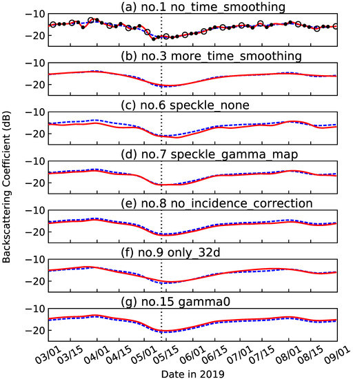
Figure 3.
Examples of BSC time-series data. The solid lines in panels (a–g) represent the spline interpolation data used in the analysis under settings no. 1, 3, 6, 7, 8, 9, and 15 shown in Table 3, respectively. The dashed lines are the spline interpolation data obtained with the default settings. The white circles in the panel (a) indicate the data of the incident angle of 32°, and the black dots indicate the data with incident angles of 41° or 45° before the spline interpolation. The vertical dashed line indicates the transplanting date block value of the target pixel in block 15.
The AVG and STD of the transplanting date estimation errors obtained under each setting are summarized in Table 4. In addition, to make it easier to understand how AVG and STD change depending on the settings for transplanting date estimation, the amount of difference in AVG and STD from the default setting were calculated and entered in the AVG dif. and STD dif. columns of Table 4, respectively.
Table 4.
Transplanting date estimation errors.
First, focusing on the STD, which cannot be corrected because it is a random error, the optimal setting was adopted for each option from A to H based on the following consideration. The results indicated that the default setting was the most optimal.
- A: Smoothening in the time direction had a strong improvement effect of approximately 0.7 days on the STD. It is considered that this is because the noise is reduced by smoothening; however, it is also considered that the restriction of the upper limit value of the BSC increases owing to the upward shifting of the BSC at the local minimum by smoothening. The stronger the smoothening, the smaller the STD tends to be. However, if the smoothening is very strong, the distortion of the time-series data becomes larger and the preliminary estimation is delayed from approaching the final estimation. Therefore, an intermediate strength, psm = 0.01 is adopted here.
- B: The spread width in the space direction showed a strong improvement effect of approximately 0.4 days on the STD. The wider the spread, the smaller the STD tended to be; however, this result may be influenced by the assumption at the test site that same block has same transplanting dates. Since such an assumption is not always correct outside the test site, an intermediate value of σl = 30 m is adopted for the spatial spread width.
- C: Moderate improvement effect of approximately 0.2 days was observed in the STD using the speckle filter. Here, the Lee filter, which gave the smallest STD, was adopted.
- D: The STD increased significantly (approximately 0.9 days) when only the data with an incident angle of 32° was used. When the data with all incident angles were used, the incident angle correction had a weak improvement effect of approximately 0.02 days on the STD. Here, a method of using data with all incident angles after performing incident angle correction was adopted.
- E: The upper limit of the BSC at the time of transplantation had an effect of approximately 0.2 days on STD. In principle, the smaller the upper limit value is, the smaller the STD becomes. However, if the upper limit value is significantly small, a signal below the upper limit value may not be found at the time of transplantation and the transplanting date may not be identified. Therefore, an intermediate value of vth = −13 dB is adopted in this study. For setting no. 11 with vth = −15 dB, there were two fields for which the transplanting dates could not be identified. Here, just one upper limit is set; however, it is also possible to set two upper limits and apply the second upper limit (vth = −13 dB) to the fields where the transplanting dates cannot be identified by the first upper limit (vth = −15 dB).
- F: By averaging the BSC around the transplanting date, there was a weak improvement effect of approximately 0.01 days on the STD. There was almost no difference in the STD when comparing the cases where the average period was ±10 days and ±20 days; however, ±20 days was adopted as the average period because a longer period makes it easier to determine the latest transplanting date when performing preliminary estimation.
- G: For the BSC, σ0 was used because the STD was small; however, the difference between the STDs of σ0 and γ0 is not significant (approximately 0.003 days). It is noted that in the case of a paddy field near a steep slope, such as Bali island, using γ0 may improve the estimation accuracy.
- H: As for the field average, the STD was smaller by approximately 0.04 days in the case of averaging the transplanting date estimated for pixels within the field than in the case of estimating the transplanting date using the BSC averaged for each field. In this study, the method of averaging the estimated transplanting date for pixels in the field by weighting the synthesized signal intensity was adopted since the STD was the smallest. Although not adopted here, the method using the BSC averaged for each field is faster and has acceptable accuracy; hence, it is a useful method when it is required to reduce the calculation time.
The following is a discussion on AVG dif. in Table 4. In most settings, AVG dif. was in the range of –0.08 days to +0.06 days; however, when there was no spatial spread (setting no. 4, Table 4) or when only the data with an incident angle of 32° was used (setting no. 9, Table 4), a relatively large AVG dif of +0.20 days or –0.30 days, respectively, was observed. This may have been due to the influence of signals other than transplantation or noise. The effect of temporal smoothing on the AVG is particularly large. The AVG dif. became +0.75 days when smoothing out in the time direction was not performed (setting no. 1, Table 4), which is considered to be caused by the unstable position of the local minimum due to the noise. Furthermore, when smoothing was weak (setting no. 2, Table 4) and strong (setting no. 3, Table 4), AVG dif. was –0.73 days and +1.02 days, respectively. This is probably because the stronger the smoothing, the more distorted the asymmetrical curve. If the settings such as the strength of the smoothing out are fixed, the value of AVG does not change much even if the cropping period is different. Therefore, in the following discussion, unless otherwise stated, a uniform offset is subtracted from the estimated transplanting date for correction. The offset value was determined to be nine days, considering the transplanting date estimation error (details will be described later) obtained for four cropping periods from March 2018 to February 2020.
3.2. Examination of Validity
3.2.1. Comparison with NDVI
The transplanting date of the first crop in the dry season of 2019 in the Cihea irrigation district was estimated pixel by pixel, and the maps of the resulting transplanting date estimation and synthesized signal intensity are shown in Figure 4a,b, respectively. The transplanting date search period was set between 1 March 2019 and 15 June 2019. Here, only the pixels interpreted to be the paddy fields were extracted by a supervised classification using BSC time-series data. Figure 4b shows that the synthesized signal intensity varies considerably from location to location; hence, it is difficult to set a uniform threshold for the synthesized signal intensity. It is estimated that, in the study area, the transplantations were performed from early March to early June in 2019. Figure 4c is a map of NDVI calculated from atmospherically corrected surface reflectance data (L2A) acquired by the Sentinel-2 satellite. The data acquisition date was 9 June 2019, three months after the transplanting in early fields (early March) and immediately after the transplanting in late fields (early June). In general, it is known that the NDVI of rice is lowest immediately after transplanting with low vegetation density, increases gradually and becomes highest around the heading time when leaves grow thick, and then gradually decreases toward the ripening stage [9]. The solid line in Figure 4d shows the relationship between the NDVI of the entire study area calculated from the Sentinel-2 image on 9 June 2019 and the number of days elapsed from the estimated transplanting date. Furthermore, the dashed line in Figure 4d shows the relationship between the NDVI in the test site calculated from multiple Sentinel-2 images acquired between April and September 2019 and the number of days elapsed from the block value of the transplanting date. In both cases, the peak of the NDVI is approximately 55 days after the transplanting date, and both the curves are similar. Therefore, it is considered that the estimation of the transplanting date for the entire study area was performed well.
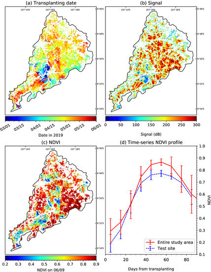
Figure 4.
Comparison of estimated transplanting date and NDVI after transplantation (first crop in the dry season of 2019). Panels (a,b) show final estimation of the transplanting date and synthesized signal intensity obtained for each pixel in the study area, respectively. Panel (c) shows the NDVI calculated from the Sentinel-2 data acquired on 9 June 2019. The solid line in panel (d) shows the time-series profile of NDVI obtained using the estimated transplanting date in the study area and the NDVI of one scene (9 June 2019), while the dashed line shows the time-series profile of NDVI obtained using the block value of transplanting date in the test site and multi-scene NDVI acquired from April 2019 to September 2019.
3.2.2. Comparison with Block Value
The transplanting date of the first crop in the dry season of 2019 in the test site was estimated for each field, and the maps of the resulting transplanting date estimation and field average signal intensity are shown in Figure 5a,b, respectively. The transplanting date search period was set between 15 March 2019 and 15 June 2019. Figure 2 and Figure 5a show similar differences in transplanting dates for different blocks; however, the estimates in Figure 5a show some variability within the same block. In Figure 5b, the field average signal intensity is low, particularly around the road inside the test site.
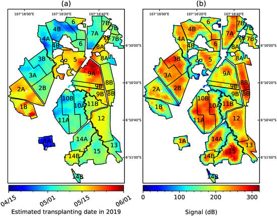
Figure 5.
Maps of estimated transplanting date (a) and field average signal intensity (b) (first crop in the dry season of 2019).
A map and a histogram of the estimation error of the transplanting date are shown in Figure 6a,b, respectively. In Figure 6a, it can be seen that the regions where the estimation error was large were often clustered in a part of blocks 4A, 4B, and 8A. In the rainy season, there is a possibility that the transplanting date in a large area can be miscalculated due to the influence of rainfall; however, since the estimated transplanting date corresponded to the dry season, the influence of rain is unlikely. There is a high possibility that the actual transplanting date for these fields was different from the block value owing to the factors such as the availability of irrigation water. Such a large deviation appears as an outlier in the histogram (Figure 6b); however, except for the deviation, the distribution is more-or-less Gaussian. Comparing Figure 5b and Figure 6a, it can be seen that the same level of estimation accuracy as the field average signal intensity of 200 dB or more can be obtained even at the field average signal intensity of approximately 100 dB.
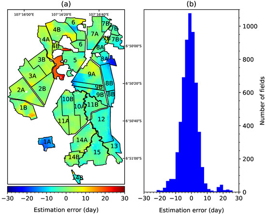
Figure 6.
Map (a) and histogram (b) of transplanting date estimation errors (first crop in the dry season of 2019).
The AVG and STD of the estimation error obtained by the similar transplanting date estimation are summarized in Table 5 for four cropping periods from March 2018 to February 2020, in which the block value of the transplanting date was available. The AVG is within ±2 days and the STD is approximately 5–6 days. The STD for the period 1 November 2018 to 1 February 2019 is as large as ~7 days; however, this period is in the rainy season, and it is possible that the period was mistakenly estimated as the transplanting period when the paddy field was flooded owing to rainfall. When all the periods were combined, the AVG estimation error was −0.33 days and the STD was 5.93 days.
Table 5.
Average and standard deviation of the transplanting date estimation errors. Dates are in YYYY/MM/DD format.
Figure 7 shows a graph in which the estimation results for these four periods are combined and the abscissa indicates the absolute value of the estimation error (allowable error), and the ordinate indicates the percentage of the estimation error within the allowable error (accuracy rate). The accuracy rates for allowable errors of 5, 10, and 15 days are 69%, 92%, and 97%, respectively.
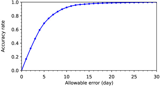
Figure 7.
Accuracy rate of estimated transplanting date (March 2018–February 2020).
In the discussion so far, the block value was regarded as the true value; however, the transplanting dates within the block were not actually uniform, and it was assumed that the spread was approximately three days. Assuming that the root mean square error of the block value was three days, the contribution of the estimated transplanting date error in the estimation error of 5.93 days was calculated to be approximately five days.
3.2.3. Difference between the Preliminary and Final Estimations
Figure 8 shows the difference between the preliminary and final estimates of the transplanting date (preliminary estimation error) for each field in the first crop of the dry season of 2019. Preliminary estimates were calculated for all the Sentinel-1 data (30 images) acquired during the period from 1 March 2019 to 1 July 2019, each of which was regarded as the latest data. The length of the transplanting search period was set to 60 days (see Section 2.2.4 for details). For the final estimation, the transplanting date search period was set from 15 March 2019 to 15 June 2019. The horizontal axis in Figure 8 is the number of days from the transplanting date (the final estimation of the transplanting date corrected for the offset of nine days) to the acquisition date of the data used for the preliminary estimation. Here, only fields where the field average signal intensity exceeded a threshold value (128 dB) were selected. This threshold value was adjusted from the final estimation result such that 90% of the fields in the test site had a field average signal intensity exceeding the threshold value. The solid line in Figure 8 shows the AVG of the preliminary estimation error, the error bar shows the STD, and the broken line shows the percentage of fields selected in the test site. The preliminary estimation gradually approaches the final estimation from ~20 days before the transplanting date, because the BSC of the field begins to decrease reflecting changes in field conditions. During this time, the percentage of the selected fields increases and approaches 90% around the transplanting date. Approximately ten days after transplantation, the preliminary estimation almost matches the final estimation. For the next several days, the preliminary estimation increases slightly because the smoothed out BSC time-series data continues to decrease; however, the preliminary estimation approaches the final estimation again after a local minimum appears in the time-series data. Therefore, the preliminary estimation is expected to be almost the same as the final estimation 10–15 days after the transplanting date.
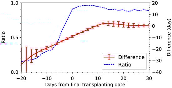
Figure 8.
Difference between the preliminary and final estimations (first crop in the dry season of 2019). The solid line shows the average of the preliminary estimation error (Preliminary estimation–Final estimation), and the error bar shows the standard deviation. Here, only fields in which the field average signal intensity exceeds the threshold (128 dB) were selected. The dashed line indicates the percentage of the selected field.
In the future, by obtaining the final estimation for each cropping period and accumulating the results of transplanting date estimation, it will be possible to understand how small the BSC at the transplanting date will be for each field. As the smoothed out BSC time-series decrease almost linearly before the transplanting date, by determining how small the BSC will be as the transplanting date approaches, it is possible to partially predict the transplanting date in advance, and a plausible preliminary estimation can be obtained at an earlier stage. Moreover, the difference between the field average signal intensity obtained by a new estimation and the past AVG value is considered to be useful as an index of the validity of the transplanting date estimation result. In other words, if the field average signal intensity obtained by a transplanting date estimation is significantly different from the past AVG value, the obtained transplanting date estimation value could be uncertain.
4. Conclusions
In Indonesia, an agricultural insurance system is in place to help paddy rice producers who suffer damages from floods, droughts, pests, and diseases. Since damage assessments by field surveys require considerable resources such as time and labor, more efficient techniques using remote sensing technology are required. In this study, we developed a method to estimate the date of rice transplanting using the VH polarization BSCs of the Sentinel-1 satellite, which can be acquired regardless of weather, have high temporal and spatial resolution, and are widely available. As a result of examining the effect on the estimation accuracy by changing the settings of the transplanting date estimation, it was found that the accuracy was mainly improved by smoothing out the time-series data, the application of a speckle filter, and by signal synthesis of the surrounding field. In addition, taking advantage of the fact that three types of Sentinel-1 data with different incident angles can be acquired for the study area, a better accuracy was obtained using the data with all the incident angles (with correction of the incident angle dependence of BSC). The STD of the estimation error was found to be approximately 5–6 days, which is smaller than nine days, i.e., the estimation error of transplanting date obtained using TerraSAR-X data [20]. The accuracy rates were 69%, 92%, and 97%, when the allowable range of estimation error was within 5, 10, and 15 days, respectively. It was confirmed that the preliminary estimation, which was updated each time new Sentinel-1 data were obtained, converged to an accurate final estimation 10–15 days after the transplanting date. In this method, the transplanting date estimation and all the necessary computational processes, from downloading to analyzing the data, were performed via Python scripts; as such, transplanting date estimations can be completely automated using a scheduler. This method takes into consideration the characteristics of the study area, and fulfills requirements such as simplicity, rapidity, and accuracy. Therefore, it can contribute to reducing the labor required and improving the efficiency for damage assessments of rice paddy fields.
Author Contributions
Conceptualization, N.M. and C.H.; methodology, N.M.; software, N.M.; validation, N.M., Y.S., G.S. and B.U.; formal analysis, N.M.; investigation, N.M., Y.S., G.S. and B.U.; resources, C.H.; data curation, N.M. and Y.S.; writing—original draft preparation, N.M.; writing—review and editing, N.M. and C.H.; visualization, N.M.; supervision, C.H.; project administration, C.H.; funding acquisition, C.H. All authors have read and agreed to the published version of the manuscript.
Funding
This research was supported by Science and Technology Research Partnership for Sustainable Development (SATREPS, Grant Number: JPMJSA1604); Japan Science and Technology Agency (JST) / Japan International Cooperation Agency (JICA).
Acknowledgments
We would like to thank Hiroaki Kuze and Hiroyuki Wakabayashi for their very useful advice in reviewing and refining the draft of the manuscript.
Conflicts of Interest
The authors declare no conflict of interest.
References
- United Nations, Department of Economic and Social Affairs, Population Division. World Population Prospects: The 2015 Revision, Key Findings and Advance Tables; Working Paper No. ESA/P/WP.241; United Nations: New York, NY, USA, 2015; p. 2. [Google Scholar]
- Food and Agriculture Organization of the United Nations. Food Outlook-Biannual Report on Global Food Markets; FAO: Rome, Italy, 2020; pp. 24–29. [Google Scholar]
- Contribution of Working Groups I, II and III to the Fifth Assessment Report of the Intergovernmental Panel on Climate Change. Climate Change 2014: Synthesis Report; Core Writing Team, Pachauri, R.K., Meyer, L.A., Eds.; IPCC: Geneva, Switzerland, 2014; pp. 55–74. [Google Scholar]
- Dewi, N.; Kusnandar; Rahayu, E.S. Risk mitigation of climate change impacts on rice farming through crop insurance: An analysis of farmer’s willingness to participate (a case study in Karawang Regency, Indonesia). In Proceedings of the International Conference on Climate Change (ICCC 2018), Solo City, Indonesia, 27–28 November 2018. [Google Scholar]
- Mutaqin, D.J.; Usami, K. Smallholder Farmers’ Willingness to Pay for Agricultural Production Cost Insurance in Rural West Java, Indonesia: A Contingent Valuation Method (CVM) Approach. Risks 2019, 7, 69. [Google Scholar] [CrossRef]
- Yanuarti, R.; Aji, J.M.M.; Rondhi, M. Risk aversion level influence on farmer’s decision to participate in crop insurance: A review. Agric. Econ.—Czech. 2019, 65, 481–489. [Google Scholar] [CrossRef]
- Fadhliani, Z.; Luckstead, J.; Wailes, E.J. The impacts of multiperil crop insurance on Indonesian rice farmers and production. Agric. Econ. 2018, 50, 15–26. [Google Scholar] [CrossRef]
- Caasi, O.; Hongo, C.; Wiyono, S.; Giamerti, Y.; Saito, D.; Homma, K.; Shishido, M. The potential of using Sentinel-2 satellite imagery in assessing bacterial leaf blight on rice in West Java, Indonesia. J. ISSAAS 2020, 26, 1–16. [Google Scholar]
- Wang, J.; Yu, K.; Tian, M.; Wang, Z. Estimation of rice key phenology date using Chinese HJ-1 vegetation index time-series images. In Proceedings of the 2019 8th International Conference on Agro-Geoinformatics (Agro-Geoinformatics), Istanbul, Turkey, 16–19 July 2019. [Google Scholar]
- Tsujimoto, K.; Ohta, T.; Hirooka, Y.; Homma, K. Estimation of planting date in paddy fields by time-series MODIS data for basin-scale rice production modeling. Paddy Water Environ. 2019, 17, 83–90. [Google Scholar] [CrossRef]
- Liu, C.; Chen, Z.; Shao, Y.; Chen, J.; Hasi, T.; Pan, H. Research advances of SAR remote sensing for agriculture applications: A review. J. Integr. Agric. 2019, 18, 506–525. [Google Scholar] [CrossRef]
- Lopez-Sanchez, J.M.; Cloude, S.R.; Ballester-Berman, J.D. Rice Phenology Monitoring by Means of SAR Polarimetry at X-Band. IEEE Trans. Geosci. Remote. Sens. 2012, 50, 2695–2709. [Google Scholar] [CrossRef]
- Tian, H.; Wu, M.; Wang, L.; Niu, Z. Mapping Early, Middle and Late Rice Extent Using Sentinel-1A and Landsat-8 Data in the Poyang Lake Plain, China. Sensors 2018, 18, 185. [Google Scholar] [CrossRef] [PubMed]
- He, Z.; Li, S.; Wang, Y.; Dai, L.; Lin, S. Monitoring Rice Phenology Based on Backscattering Characteristics of Multi-Temporal RADARSAT-2 Datasets. Remote Sens. 2018, 10, 340. [Google Scholar] [CrossRef]
- Singha, M.; Dong, J.; Zhang, G.; Xiao, X. High resolution paddy rice maps in cloud-prone Bangladesh and Northeast India using Sentinel-1 data. Sci. Data 2019, 6, 1–10. [Google Scholar] [CrossRef] [PubMed]
- Wakabayashi, H.; Motohashi, K.; Kitagami, T.; Tjahjono, B.; Dewayani, S.; Hidayat, D.; Hongo, C. Flooded Area Extraction of Rice Paddy Field in Indonesia Using SENTINEL-1 SAR Data. ISPRS—Int. Arch. Photogramm. Remote. Sens. Spat. Inf. Sci. 2019, XLII-3/W7, 73–76. [Google Scholar] [CrossRef]
- Li, M.; Bijker, W. Vegetable classification in Indonesia using Dynamic Time Warping of Sentinel-1A dual polarization SAR time series. Int. J. Appl. Earth Obs. Geoinf. 2019, 78, 268–280. [Google Scholar] [CrossRef]
- Nurtyawan, R.; Saepuloh, A.; Harto, A.B.; Wikantika, K.; Kondoh, A. Satellite Imagery for Classification of Rice Growth Phase Using Freeman Decomposition in Indramayu, West Java, Indonesia. HAYATI J. Biosci. 2018, 25, 126–137. [Google Scholar]
- Lestari, A.I.; Kushardono, D. The use of C-band synthetic aperture radar satellite data for rice plant growth phase identification. IJReSES 2019, 16, 31–44. [Google Scholar] [CrossRef]
- Asilo, S.; de Bie, K.; Skidmore, A.; Nelson, A.; Barbieri, M.; Maunahan, A. Complementarity of Two Rice Mapping Approaches: Characterizing Strata Mapped by Hypertemporal MODIS and Rice Paddy Identification Using Multitemporal SAR. Remote Sens. 2014, 6, 12789–12814. [Google Scholar] [CrossRef]
- Nguyen, D.B.; Gruber, A.; Wagner, W. Mapping rice extent and cropping scheme in the Mekong Delta using Sentinel-1A data. Remote Sens. Lett. 2016, 7, 1209–1218. [Google Scholar] [CrossRef]
- Nguyen, D.B.; Wagner, W. European Rice Cropland Mapping with Sentinel-1 Data: The Mediterranean Region Case Study. Water 2017, 9, 392. [Google Scholar] [CrossRef]
- de Boor, C.A. Practical Guide to Spline; Springer: New York, NY, USA, 1978. [Google Scholar]


Publisher’s Note: MDPI stays neutral with regard to jurisdictional claims in published maps and institutional affiliations. |
© 2020 by the authors. Licensee MDPI, Basel, Switzerland. This article is an open access article distributed under the terms and conditions of the Creative Commons Attribution (CC BY) license (http://creativecommons.org/licenses/by/4.0/).