Abstract
pH value is a crucial indicator for evaluating silage quality. In this study, taking maize silage as the research object, a quantitative prediction model of pH value change during the secondary fermentation of maize silage was constructed based on computer vision. Firstly, maize silage samples were collected for image acquisition and pH value determination during intermittent and always-aerobic exposure. Secondly, after preprocessing the acquired image with the region of interest (ROI) interception, smoothing, and sharpening, the color and texture features were extracted. In addition, Pearson correlation analysis and RF importance ranking were used to choose useful feature variables. Finally, based on all feature variables and useful feature variables, four regression models were constructed and compared using random forest regression (RFR) and support vector regression (SVR): RFR model 1, RFR model 2, SVR model 1, and SVR model 2. The results showed that—compared with texture features—the correlation between color features and pH value was higher, which could better reflect the dynamic changes in pH value. All four models were highly predictive. The RFR model represented the quantitative analysis relationship between image information and pH value better than the SVR model. RFR model 2 was efficient and accurate, and was the best model for pH prediction, with , , RMSEC, RMSEP, and RPD of 0.9891, 0.9425, 0.1758, 0.3651, and 4.2367, respectively. Overall, this study proved the feasibility of using computer vision technology to quantitatively predict pH value during the secondary fermentation of maize silage and provided new insights for monitoring the quality of maize silage.
1. Introduction
Maize silage has become the main roughage used in ruminants’ diets, especially for dairy cattle diets worldwide [1,2]. Ensiling is a method for the long-term preservation of the nutritional characteristics of green fodder [3]. It is based on solid-state lactic acid fermentation under anaerobic conditions whereby lactic acid bacteria (LAB) convert water-soluble sugars into organic acids, mainly to lactic acid, which lowers the pH value of silage and inhibits the growth of spoilage microorganisms so that green crops can be preserved [3]. The ensiling process can be divided into four phases: (i) initial aerobic phase, (ii) fermentation phase, (iii) stable phase/storage phase, and (iv) feeding out phase/aerobic deterioration phase [4,5]. Among them, pH value is a crucial indicator for evaluating silage quality that can reflect whether the silage is well preserved and the degree of its decomposition by spoilage bacteria [6]. The pH value of well-preserved silage is generally around 3.7–4.0 [7]. However, when the silage wrapping-plastic film is damaged, the silage seal is not tight, and the silage silo is opened for feeding, the silage will inevitably be exposed to the air, and the oxygen in the air will invade the feed through the exposed surface, which will lead to the rapid proliferation of aerobic microorganisms (such as yeasts and molds, etc.), resulting in secondary fermentation of silage, which will in turn lead to the increase of pH value in the feed, the loss of nutrients, and finally the aerobic deterioration of silage [5,8]. Moreover, the growth of molds may produce mycotoxins, which threaten the health of humans and animals [9]. Therefore, accurate detection of pH changes during maize silage secondary fermentation can clarify their degree of aerobic deterioration, thus optimizing feed ensiling production methods, improving its fermentation quality, and promoting the healthy development of the animal husbandry industry.
At present, the main method for detecting the pH value of maize silage is laboratory determination. The detection results of this method are accurate, and the error is relatively small, but there are some problems, such as cumbersome detection procedures, time needed, high cost, and damaged samples [10]. Therefore, it is urgent to develop a new method for rapid, accurate, and nondestructive detection of maize silage pH value. Near-infrared spectroscopy (NIRS) and computer vision, common nondestructive testing techniques, have been applied in many fields.
NIRS is now a favored analytical technique because it is fast, low-cost, and nondestructive with no requirements for solvents or reagents, which can replace the wet analysis to describe the preservation quality of silage [10,11]. Sørensen et al. [12] used near-infrared (NIR) spectroscopy to develop predictive models for the determination of lactic acid (Lac), acetic acid (HAc), pH, NH3 N, and ethanol (EtOH) in grass and corn silages. Liu et al. [13] established a quantitative analysis model for pH value and fermentation products (lactic acid, acetic acid, propionic acid, butyric acid, and ammonia nitrogen) of straw silage by near-infrared spectroscopy combined with partial least squares (PLS) regression. Park et al. [14] established a regression model of chemical composition and fermentation parameters in maize silage by near-infrared spectroscopy combined with partial least squares (PLS) multivariate analysis. The model accuracy was improved by mathematical transformation, and the correlation coefficient of cross-validation was 0.74–0.91. Hetta et al. [15] used a high-quality near-infrared (NIR) spectrometer and an NIR hyperspectral imaging technique using partial least squares (PLS) regression models to predict the nutritive, morphological, and agronomic characteristics of forage maize. It was found that the technology had robust results for predicting CP, starch, WSC, and maize ear proportions.
Computer vision is a bionic technology that simulates visual functions to obtain information about the color, texture, and shape of tested samples [16]. As information science is rapidly growing, computer vision-based pattern recognition and image processing are widely used in agricultural safety and quality analysis [17], such as weed and disease detection [18,19], maturity classification [20,21,22], variety identification [23,24], and quality inspection [25,26,27]. Sanaeifar et al. [28] used color features in different color spaces as the inputs of the model and used support vector regression (SVR) and an artificial neural network (ANN) to establish a quantitative prediction model for changes in total soluble solids, pH, titratable acidity, and firmness during banana storage. The results indicated that the support vector regression (SVR) model with the radial basis function (RBF) as the kernel function had higher prediction accuracy than the results obtained using the artificial neural network (ANN). Dong et al. [29] established linear and nonlinear quantitative evaluation models of physicochemical indexes (TFs, TRs, and TBs) and sensory features using color-feature parameters as inputs. The results suggested that color features were significantly correlated to quality indices. The predictability of nonlinear models (RF and SVM) was superior to the PLS linear model, while the RF model presented a slight advantage over the classic SVM model. Sabzi et al. [30] developed a three-variety automatic and nonintrusive computer vision system to estimate orange fruit pH value, and the regression coefficients for pH estimation in Bam, Blood, and Thomson orange varieties, were 0.950, 0.935, and 0.957, respectively. Keramat-Jahromi et al. [31] built an online imaging system for date fruit chips and designed a moisture ratio (MR) regression model for date fruit chips using random forest (RF) and k-nearest neighbor (kNN) algorithms with r2 of 0.976 and 0.959 in the test set, respectively, and found a correlation between the color change and moisture content of date fruits.
Vision-based sensory evaluation plays an essential role in evaluating maize silage quality [32]. However, there are few literature reports on the quantitative prediction of maize silage pH value by computer vision technology. Most of the research has focused on the quantitative analysis of silage fermentation and nutritional quality indicators using near-infrared spectroscopy. In addition, the correlation and quantitative analysis relationship between image features and the pH value of maize silage are unclear.
Therefore, this study aimed to explore the feasibility of predicting the pH value during maize silage secondary fermentation based on computer vision technology. The specific research objectives included (1) analyzing the relationship between pH value and image features during the secondary fermentation, (2) studying the changes in pH value and image features during the secondary fermentation, (3) screening the optimal feature variable set, and (4) establishing a quantitative prediction model of pH value with good accuracy and high efficiency.
2. Materials and Methods
2.1. Sample Preparation
The experiment was conducted from September 2021 to January 2022. Maize (variety: Jinling Silage 357, Inner Mongolia Jinling Maize Silage Seed Industry Co., Ltd., Chifeng, China) was planted in Donghuaying Village (111° E, 40° N), Tumd Left Banner, Hohhot, Inner Mongolia Autonomous Region, China. It was harvested from the late milk stage to the early dough stage (more than 2/3 of the maize milk line). Using a self-propelled forage harvester (Muze 4QZ-18A, Hebei Muze Animal Husbandry Machinery Co., Ltd., Shijiazhuang, China) to harvest the whole maize plants, chop it to 1–2 cm, and wait for ensilage. Maize silage preparation, sample treatment, and pH determination were all carried out in the Laboratory of Agricultural Mechanization Engineering Discipline (111°43′ E, 40°49′ N) of Inner Mongolia Agricultural University, China.
On the day of maize harvest (14 September 2021), the chopped maize was immediately packed into polyethylene bags (50 cm × 70 cm) and plastic buckets (10 L), compacted and sealed, wrapped in multiple layers of preservative films, and stored at room temperature (18–26 °C) away from light. After 60 days of ensiling, the fermentation of the maize silage was stable, and the ensilage ended.
After the ensilage was finished, 165 high-quality maize silage samples were randomly collected from different silage preparation devices. When sampling, first remove the silage material layer of 10–15 cm from the top, bottom, left, and right, and then evenly select three sampling points on the upper, middle, and lower layers of the silage material, each sampling point to take about 250 g silage, which was put into vacuum bags, and vacuum sealed. The collected samples can be analyzed immediately or stored in the refrigerator at 4 °C until further processing.
In order to simulate the secondary fermentation caused by the open feeding of the silage silo (intermittent invasion of oxygen) or the damage of the silage wrapping-plastic film (constant attack of oxygen), three different treatments were carried out on the collected samples, as follows:
- (1)
- No aerobic exposure treatment: 40 samples were randomly selected from the collected samples for direct analysis.
- (2)
- Intermittent aerobic exposure treatment: 75 samples were randomly selected from the collected samples, opened in 1–15 days, opened for 1 h every day, and placed in polystyrene boxes with several holes (10 mm in diameter) around them. Then, the lid was covered to reduce moisture evaporation. This process was carried out at room temperature (18–22 °C), and five samples were randomly taken daily for analysis.
- (3)
- Always-aerobic exposure treatment: 50 samples were randomly selected from the collected samples, kept unsealed for 1–10 days, placed in polystyrene boxes with several holes, and covered with lids. This process was carried out at room temperature (18–22 °C), and five samples were randomly taken daily for analysis.
As such, a total of 165 samples were collected during the maize silage secondary fermentation. Image acquisition and pH determination were performed on the collected samples for testing. The experimental and data analysis process is shown in Figure 1.
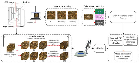
Figure 1.
Experiment and data analysis flowchart.
2.2. Construction of Computer Vision System
The computer vision system used in this study was mainly composed of two light sources, a camera, a computer, and a dark box (Figure 1). According to the overall system requirements, a CCD camera (BFLY-PGE-50H5C-C, Teledyne FLIR, Wilsonville, OR, USA) with a resolution of 2248 × 2048 pixels, strip LED lights (HF-TX10030, Dongguan Kemai Vision Technology Co., Ltd., Dongguan, China), a dark box painted black inside, and a computer with imaging software (FlyCapture2, Teledyne FLIR, Wilsonville, OR, USA) were finally selected in this study. The light sources were installed on both sides of the dark box, and the camera was installed on the bracket above the sample. The machine was turned on and warmed up for 30 min before image acquisition, and image acquisition was performed after the computer vision system had stabilized.
2.3. Chemical Analysis and Image Acquisition
The quartering method reduced each maize silage sample to 10 g (accurate to 0.1 g) [33], which was then placed in 300 mL glass beakers, mixed thoroughly with 90 mL of distilled water, and soaked in distilled water for 0.5 h. After soaking, each sample was filtered through four layers of cheesecloth and the pH value of the filtrate immediately measured with a pH meter (PHS-3CB, Shanghai Yueping Scientific Instrument Co., Ltd., Shanghai, China) (Figure 1) with a resolution of 0.01 and an accuracy of ±0.01. Each measurement was repeated three times, and the average of the three measurements was taken as the final pH value. The above process was carried out at room temperature (18–22 °C).
After measuring the actual pH value of each maize silage sample, we immediately mixed the remaining part of each sample evenly, randomly weighed 70 ± 0.5 g of maize silage from it, and evenly spread it in a φ 120 × 23 mm quartz petri dish. Then, after adjusting the relevant settings of the light source and CCD camera to achieve the ideal imaging effect, we sequentially acquired the images of the maize silage samples through the computer vision system. Four images were acquired each time, and the one with the best imaging quality was selected as the final sample image. A total of 165 final sample images were obtained. The acquired images were 24-bit RGB color images with a resolution of 2248 × 2048 pixels and saved in BMP format.
2.4. Image Preprocessing and Feature Extraction
The image processing algorithm was written by MATLAB software (MATLAB R2021a, MathWorks, Natick, MA, USA) to perform image preprocessing and feature extraction on the collected images (Figure 1). In order to simplify the feature extraction process and eliminate data related to image background [34], this study intercepted the 1000 × 1000 pixels region of interest (ROI) from the center of the acquired maize silage image as the target region for preprocessing and feature extraction. The median filter was used to smooth the ROI to eliminate image noise, and then the Laplacian operator was used to perform spatial convolution on the smoothed image to make the image texture clearer and more evident after noise elimination [35,36].
After image preprocessing was completed, feature extraction began. A total of 56 features were extracted from each ROI image: 30 color features and 26 texture features. The image features are shown in Table 1. As per [37], the ROI image was transformed from RGB to HSI and CIE L*a*b* color spaces, and the color features 1–26 were extracted by color moment according to [38]. Based on Ravg, Gavg, and Bavg values, color features 27–30 were extracted according to [39,40,41,42]. In order to extract texture features, ROI color images were first converted to grayscale images [34]. As per [36,43], gray image histogram statistical moment and gray level co-occurrence matrix were used to extract texture features 31–36 and 37–56. Pearson correlation analysis between image features and pH values was performed using SPSS software (Statistics 26, IBM, Armonk, NY, USA).

Table 1.
Color feature and texture feature list of maize silage image.
2.5. Data Analysis
Three of the 165 samples collected in this study were seriously reflective. After removing these three obvious outlier samples, 162 valid samples were finally obtained. To analyze the collected data, this study used two machine learning algorithms (random forest regression and support vector regression) to predict the pH value of maize silage (Figure 1). To obtain the best performance of the models, two different models were used to train and test each machine learning algorithm. The two models differ in the number of input variables and model parameters. Model 1 took all the features in Table 1 as model inputs and adjusted the hyperparameters. Since model optimization takes time, Model 2 eliminated unimportant features and adjusted the hyperparameters. This study used MATLAB R2021a for data analysis. The RF code was obtained from the random-forest MATLAB open-source toolbox. The SVR code was obtained from the libsvm toolbox (http://www.csie.ntu.edu.tw/~cjlin (accessed on 4 July 2022)) of MATLAB.
To reduce the risk of model overfitting, this study used the Kennard–Stone (K-S) algorithm [44] to divide the collected 162 valid samples into two sets at a ratio of 4:1:130 samples (calibration set), which were used to calibrate the models and for cross-validation (CV), while the remaining 32 samples (prediction set) were used for independent test prediction [45]. In addition, because the extracted color and texture feature variables are diversified high-dimension arrays, the dimension and order of magnitude of each variable are different [29]. To eliminate the dimension and order of magnitude restrictions, the study used the z-score normalization method [46] to preprocess the raw data, and the calculation method is shown in Equation (1):
where are the normalized data, are the raw data, μ is the arithmetic mean, and δ is the standard deviation.
K-fold cross-validation is widely applied to find the best machine learning algorithm with the best parameters due to its simple and easy properties [47]. This study used K-fold cross-validation to validate the constructed model internally. The mechanism is to create a K-fold partition for all samples in the calibration set, use K-1 folds for training, and another fold for validation, repeat the cross-validation K times, and take the mean value of the mean squared error (MSE) value of the K validations as a result, and the smaller the MSE value, the better the generalization ability of the model [16,47]. The parameter with the smallest MSE value is finally selected as the optimal parameter for the model. The above process is the training and parameter optimization process of model establishment.
2.5.1. Random Forest Regression (RFR)
Random forest (RF) is an ensemble learning algorithm with predictive classification and regression capabilities proposed by Breiman [48]. Random forest regression (RFR) is a regression version of RF [49]. The algorithm uses the bootstrap resampling method to generate multiple training sets randomly and uses each training set to generate a corresponding regression decision tree; when generating a decision tree, the segmentation variables of each node of the decision tree are generated by randomly selected few variables, and split the nodes in a best-split way [50]. In the regression process, each regression decision tree returns its prediction result, and the output of RFR is the average of the prediction results of these regression decision trees [49].
ntree and mtry are the two primary adjustment parameters in the random forest [25]. ntree is the number of decision trees, and the larger the ntree value, the better the performance of the random forest; mtry is the number of features contained in the feature subset at each decision tree split node, and the larger the mtry value, the higher the prediction performance of the model, while the diversity of the random forest will be reduced [51,52]. This study used 3-fold cross-validation combined with a grid search method (GS) to optimize the model to find the best ntree and mtry values. The parameter ranges of ntree and mtry are shown in Table 2.

Table 2.
Various parameters of RFR model.
Furthermore, random forests can determine the importance of feature variables. This study used the mean decrease in MSE built into the random forest regression model as the variable importance measure (VIM) to evaluate the degree of influence of each variable on the dependent variable [53]. Among them, the higher the VIM corresponding to the feature variable, the higher the degree of influence on the dependent variable, the more critical the feature variable is [54].
2.5.2. Support Vector Regression (SVR)
Support vector machine (SVM) is one of the most popular recent machine learning methods, and is widely used and studied for its predictive ability, not only for classification but also for regression [55]. Support vector regression (SVR) is a crucial application branch of SVM. The idea of SVR is to map the dataset to a high-dimension feature space through nonlinear mapping and then build a linear model in this space to estimate the regression function [56].
Some studies have shown that the performance of SVR is greatly affected by the kernel function form, the penalty factor (c), and the kernel parameter (g) [56]. Currently, the widely used kernel functions mainly include linear kernel function, polynomial kernel function, radial basis function (RBF), and sigmoid kernel function. The radial basis function can often get better prediction results without prior knowledge guidance. Therefore, we chose the radial basis function as the kernel function. After determining the radial basis function as the kernel function, it is also necessary to determine the penalty factor (c) and the kernel parameter (g). Parameter c minimizes the fitting error and model complexity, while parameter g defines the nonlinear mapping from the input space to the high-dimension feature space [57]. To optimize the SVR prediction model, we used a grid-search method (GS) to search for the optimal combination of (c, g) through 3-fold cross-validation. The ranges of c and g are shown in Table 3.

Table 3.
Various parameters of the SVR model.
2.6. Model Evaluation Indices
In order to evaluate the performance of the model, we introduced the decision coefficient of the calibration set (), the root mean square error of the calibration set (RMSEC), the decision coefficient of the prediction set (), the root mean square error of the prediction set (RMSEP) and the ratio of performance to deviation (RPD) to evaluate the model. The relevant calculation equations are as follows:
where is the number of samples in the calibration set, is the predicted value of the ith sample in the calibration set, is the measured value of the ith sample in the calibration set, and is the average of the measured values of all samples in the calibration set.
where is the number of samples in the calibration set, is the predicted value of the ith sample in the calibration set, and is the measured value of the ith sample in the calibration set.
where is the number of samples in the prediction set, is the predicted value of the ith sample in the prediction set, is the measured value of the ith sample in the prediction set, and is the average of the measured values of all samples in the prediction set.
where is the number of samples in the prediction set, is the predicted value of the ith sample in the prediction set, and is the measured value of the ith sample in the prediction set.
where SD is the standard deviation of the prediction set and RMSEP is the root mean square error of the prediction set.
and are used to indicate the goodness of fit of the model, with 0 indicating no correlation and 1 indicating a perfect linear relationship between predicted and measured values: the larger the value, the better the prediction performance of the model [58]. RMSEC and RMSEP evaluate the difference between predicted and measured values. The lower the value, the higher the model prediction accuracy. Moreover, the ratio of performance to deviation (RPD) is used to define the ability of the model to predict future data [59]. RPD < 1.5 indicates very poor model predictions, and its use is not recommended; RPD between 1.5 and 2 indicates poor model predictions, where only high and low values are distinguishable; RPD between 2 and 2.5 indicates fair model predictions that may be used for approximate quantitative predictions; and RPD 2.5–3.0 and above 3.0 indicates quantitative predictions can be made with good and very good predictions, respectively [60]. The higher the RPD value, the better the predictive power of the model [61].
3. Results and Discussions
3.1. Correlation between Image Features and pH Value
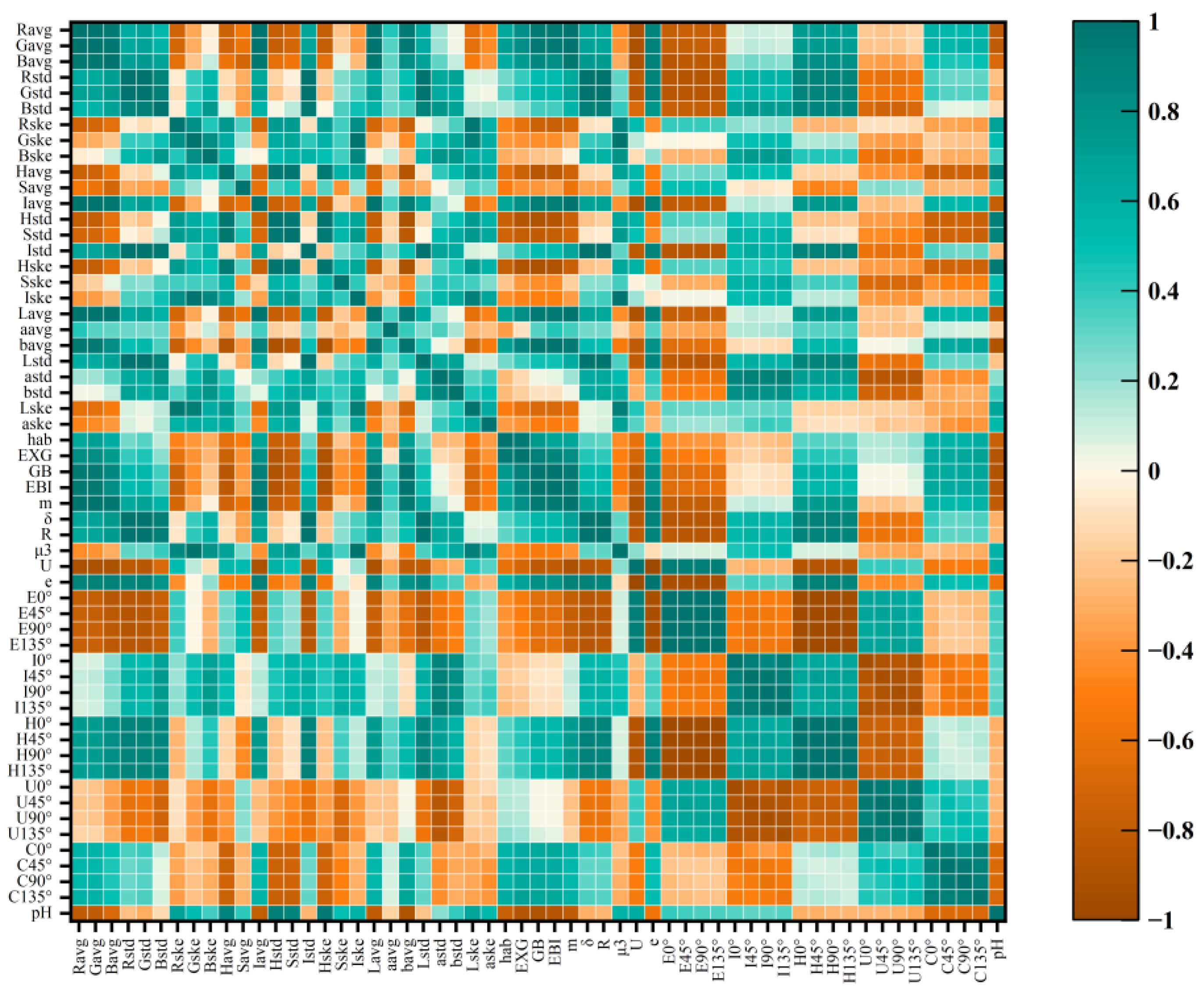
In order to obtain the best set of feature variables for predicting pH value, this study analyzed the correlation between image features and pH value by Pearson correlation analysis, as shown in Figure 2. Among the 56 image features, except for features Bstd and aavg, other features were significantly correlated with pH (p < 0.01). Among them, there are 12 image features with a high correlation with pH (Pearson correlation coefficient |r| > 0.8). These features were all color features (Hske, Hstd, Sstd, bavg, GB, Havg, EBI, EXG, Lavg, Gavg, Ravg), except for the texture feature m. The correlation coefficient between Hske and pH in the color features was as high as 0.947. This indicated that the correlation between color features and pH was more elevated than texture features, and the changes in some color features were consistent with the changes in pH. Among the 12 image features, except for the features Havg, Hstd, Hske, and Sstd, which were significantly positively correlated with pH, other features were significantly negatively correlated with pH. Since Lavg is a measure of image brightness, the color of the b* channel is from blue to yellow, and EXG is a measure of green. The lower the pH of the maize silage, the brighter it will be and the more intense the yellowish green. Thus, the color features are a good description of the dynamic changes in pH value during the maize silage secondary fermentation.
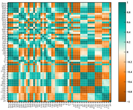
Figure 2.
Correlation chart between image features and pH value.
3.2. Changes in Image Features during Secondary Fermentation
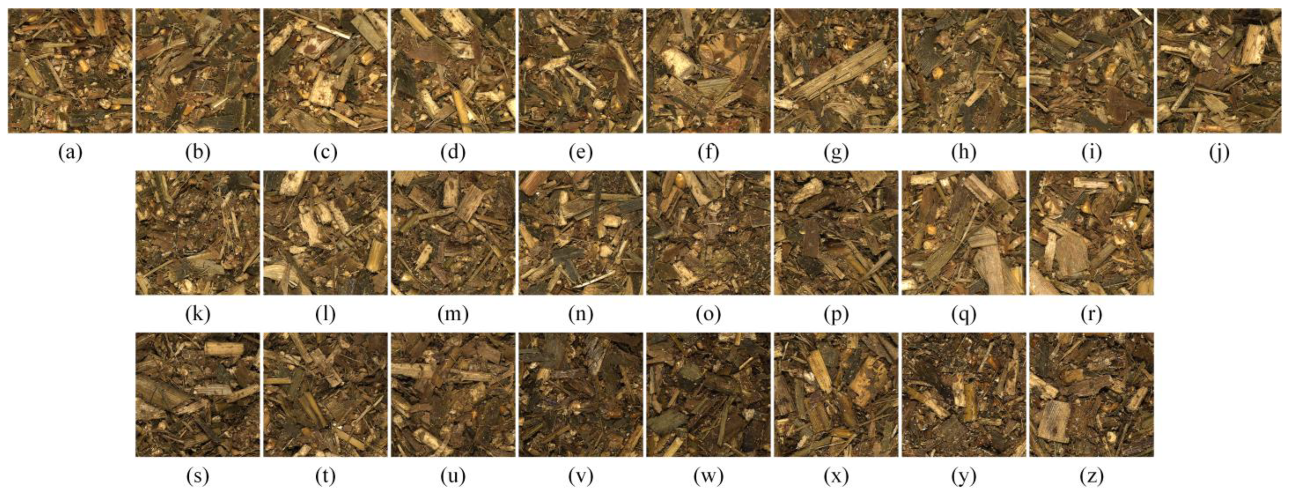
The images of the samples during the maize silage secondary fermentation are shown in Figure 3. In general, the color changes of maize silage during intermittent and always-aerobic exposure were very similar. With time, its color changed from bright yellowish green to yellowish brown, and finally to dark brown or even black, and white mildew spots appeared in the maize silage at the late stage of the always-aerobic exposure treatment.

Figure 3.
RGB images during secondary fermentation: (a) images of samples without aerobic exposure; (b–p) images of samples during intermittent aerobic exposure; (q–z) images of samples during always-aerobic exposure.
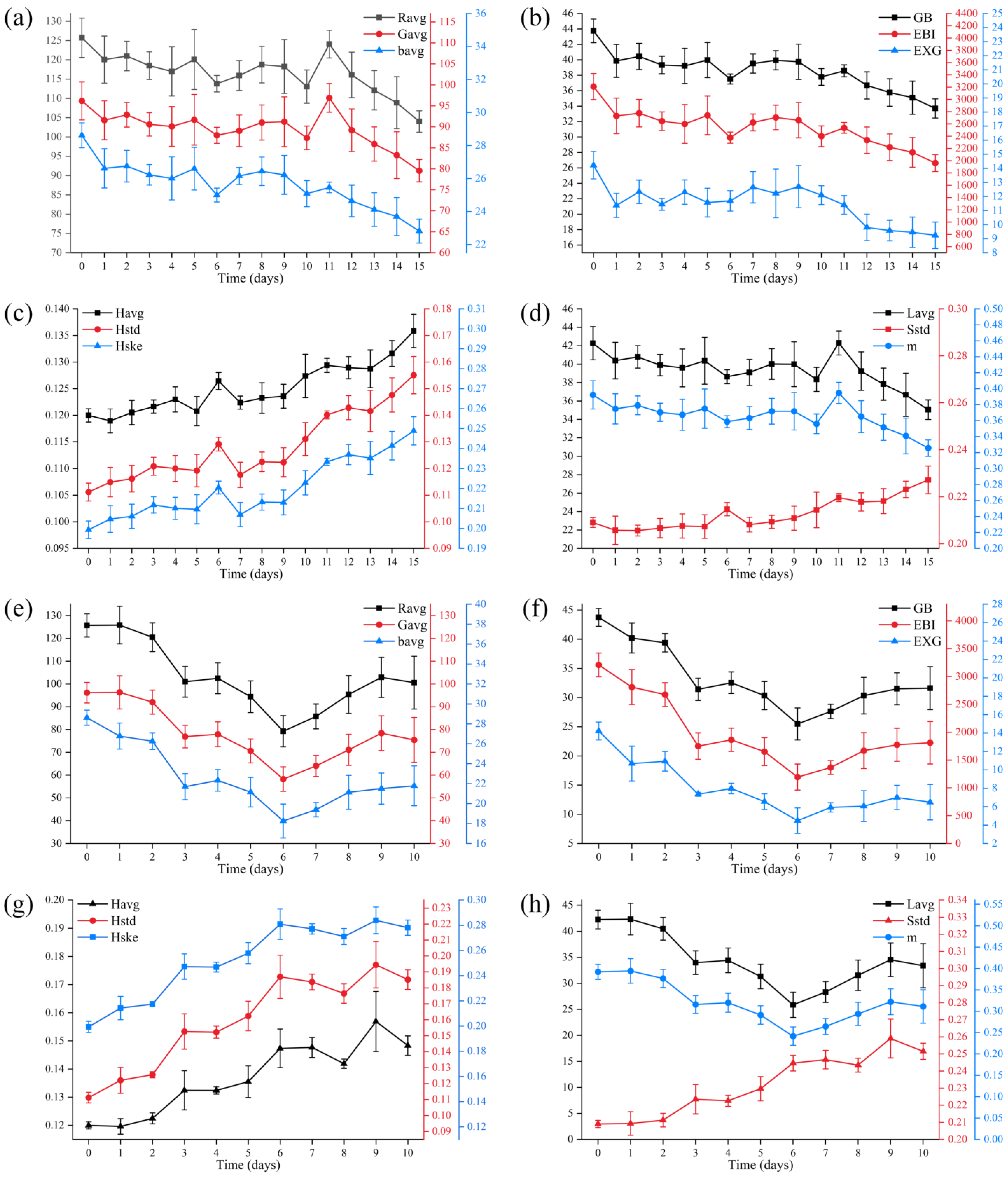
In order to evaluate the image information more objectively, this study analyzed the dynamic change law of image feature variables (highly correlated with pH value) during intermittent/always-aerobic exposure treatment, as shown in Figure 4a–h. During the intermittent aerobic exposure treatment, the changing trends of Ravg, Gavg, Lavg, bavg, and m values were roughly the same, with a slight decrease at first and then a rapid decline after 11 days. GB, EBI, and EXG values all showed a slow decrease trend, while Havg, Hstd, Hske, and Sstd values showed an upward trend from slow to fast. During the always-aerobic exposure, the changes in Ravg, Gavg, Lavg, bavg, m, GB, EBI, and EXG values were roughly the same, and decreased rapidly at the beginning and then increased slowly after 6 days, while Havg, Hstd, Hske, and Sstd values all showed an upward trend. This meant that the yellowness, greenness, and brightness of maize silage constantly decreased with intermittent aerobic exposure and always-aerobic exposure, while the yellowness, greenness, and brightness increased at the end of the always-aerobic exposure treatment, probably due to the appearance of white mildew spots. Compared with the maize silage treated with intermittent aerobic exposure, the changing trends of image feature values of the always-aerobic exposure treatment were more prominent. It showed that the color change of the maize silage samples treated with always-aerobic exposure was more intense than those treated with intermittent aerobic exposure. These results are consistent with the color changes in the sample images in Figure 3.
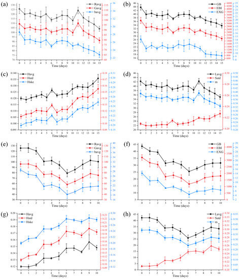
Figure 4.
Changes in image features during secondary fermentation. (a–d) Changes in image features during intermittent aerobic exposure: (a) Ravg, Gavg, bavg; (b) GB, EBI, EXG; (c) Havg, Hstd, Hske; (d) Lavg, Sstd, m; (e–h) changes in image features during always-aerobic exposure: (e) Ravg, Gavg, bavg; (f) GB, EBI, EXG; (g) Havg, Hstd, Hske; (h) Lavg, Sstd, m.
3.3. Changes in pH Value during Secondary Fermentation
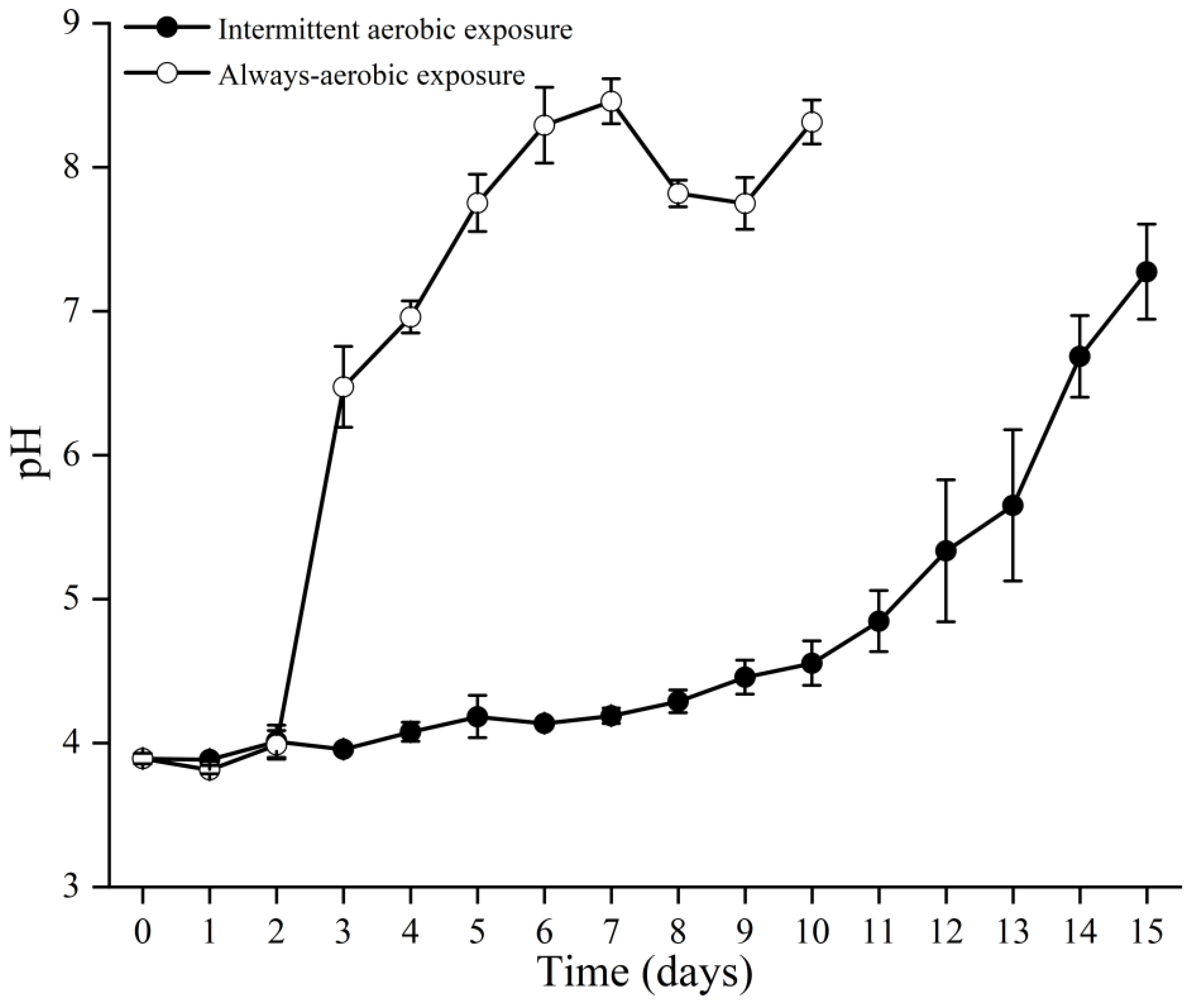
The relationship between pH value and storage time during the maize silage secondary fermentation was analyzed, as shown in Figure 5. The pH values of both the intermittent aerobic exposure treatment and always-aerobic exposure treatment groups showed an increasing trend with prolongation of storage time: compared with the intermittent aerobic exposure group, the pH value of the always-aerobic exposure group increased more quickly. It indicated that the always aerobically exposed maize silage was more likely to deteriorate. During the intermittent aerobic exposure of maize silage, the pH value showed an upward trend from slow to fast, which increased from 3.89 to 7.27. The increasing trend in pH value was slow in the first 11 days. From the 12th day, the pH value began to increase sharply, and the maize silage began to deteriorate. The pH value of maize silage treated with always-aerobic exposure changed slightly in the first 2 days. On the first day, it decreased from 3.89 to 3.81, which may be due to the increase of acetic acid content by aerobic fermentation; From the third day, it began to increase sharply, the feed became very hot, and the maize silage began to deteriorate. On the 7th day, the pH value reached a maximum of 8.46, the feed became hot for the second time, and the silage corn feed became sticky and lumpy with a foul smell. After 7 days, the pH value fluctuated in the range of 7.75–8.31, the maize silage was contaminated with molds, and the moldy smell was heavy. The first-feed fever was related to the development of yeasts and aerobic acetic acid bacteria, and the second-feed fever reflected the growth of molds [62]. The main reason for the above pH changes was the change in lactic acid content. Lactic acid is the dominant acid during silage fermentation, which can inhibit the reproduction of harmful bacteria and is the primary chemical substance for silage fermentation to enter a stable state. When the maize silage is in contact with the air, aerobic microorganisms begin to multiply, a large number of nutrients are lost from the silage, while a large amount of heat is released, resulting in an increase in the internal temperature of the feed and causing a significant reduction in lactic acid content [62], which in turn leads to an increase in pH. The above results conform with previous studies in this field [63,64].

Figure 5.
Changes in pH value during secondary fermentation.
3.4. RFR
The relative importance of image features was obtained by analyzing the data in Table 1 based on the RF method, as shown in Figure 6. The figure shows that eight color features are the most important features identified by the RF method. Hske has the highest feature importance score among these features, followed by Hstd, bavg, GB, Havg, EBI, Sstd, and EXG. Figure 2 also confirms the high correlation of these features with the pH of the maize silage. Therefore, this paper used the above eight features as the inputs of RFR model 2 to establish a simplified prediction model to shorten the model running time and improve the model prediction efficiency.
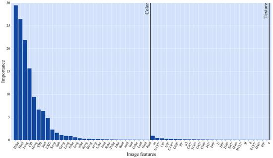
Figure 6.
Importance ranking of image features.
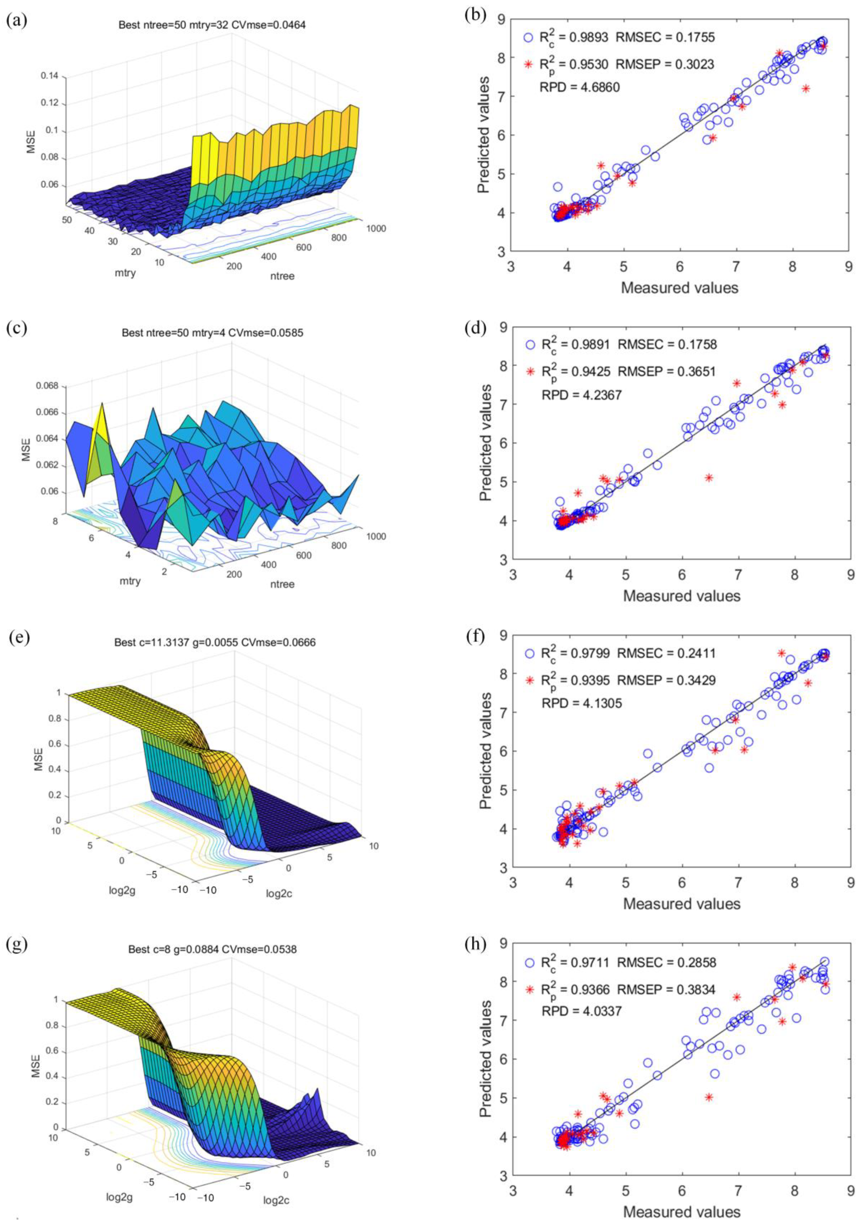
The parameter optimization process and the regression between the predicted and measured values of RFR model 1 and model 2 are shown in Figure 7a–d. In RFR model 1, when the ntree value is 50, and the mtry value is 32, the model prediction effect is the best, and its , , RMSEC, RMSEP, and RPD values are 0.9893, 0.9530, 0.1755, 0.3023 and 4.6860, respectively. In RFR model 2, when the ntree value is 50, and the mtry value is 4, the model prediction effect is the best, and its , , RMSEC, RMSEP, and RPD values are 0.9891, 0.9425, 0.1758, 0.3651, and 4.2367, respectively.

Figure 7.
Model optimization based on RFR and SVR: (a) RFR model 1 parameter optimization; (b) regression between measured and predicted values of RFR model 1; (c) RFR model 2 parameter optimization; (d) regression between measured and predicted values of RFR model 2; (e) SVR model 1 parameter optimization; (f) regression between measured and predicted values of SVR model 1; (g) SVR model 2 parameter optimization; (h) regression between measured and predicted values of SVR model 2.
3.5. SVR
The first eight features (Hske, Hstd, Sstd, bavg, GB, Havg, EBI, EXG) highly correlated with the pH value of maize silage in Figure 2 were used as model inputs to establish a simplified SVR model 2. The parameter optimization process and the regression between the predicted and measured values of SVR model 1 and model 2 are shown in Figure 7e–h. In SVR model 1, when the c value is 11.3137, and the g value is 0.0055, the model prediction effect is the best, and its , , RMSEC, RMSEP, and RPD values are 0.9799, 0.9395, 0.2411, 0.3429, and 4.1305, respectively. In SVR model 2, when the c value is 8, and the g value is 0.0884, the model prediction effect is the best, and its , , RMSEC, RMSEP, and RPD values are 0.9711, 0.9366, 0.2858, 0.3834, and 4.0337, respectively.
3.6. Model Comparison and Discussion
In order to find a more optimized modeling method to achieve rapid and accurate prediction of pH value, we compared the performance of the four models, and the results are shown in Table 4. The results showed that the RPD values of the four models were all greater than 3, indicating that the four models had good predictive ability and could be used to predict the maize silage pH value quantitatively. The RMSEP values of the RFR model prediction set were smaller than that of the SVR model, while the and RPD values were higher than that of the SVR model. Therefore, compared with the SVR model, the RFR model improves the prediction accuracy of the model. This indicated that the RFR model was very suitable for predicting the pH changes of maize silage. In addition, after removing the unimportant feature variables, the performance of both the simplified RFR and SVR models decreased due to the loss of some data, but the decrease was slight, and both the RFR and SVR models before and after the simplification showed similar prediction accuracy. Therefore, the simplified model could still meet the needs of maize silage pH prediction. Among the four models, RFR model 1 had the largest value and RPD value, and the RMSEP value was the smallest. This suggested that RFR model 1 had the best prediction performance among the four models, followed by RFR model 2, SVR model 1, and SVR model 2. RFR model 2 had a shorter running time and similar prediction accuracy to RFR model 1. Therefore, RFR model 2 was the best predictive model in this study, which achieved rapid and accurate estimation of the maize silage pH value.

Table 4.
Performance comparison of different pH value prediction models.
4. Conclusions
This study demonstrated the feasibility of using computer vision technology to predict pH quantitatively during maize silage secondary fermentation. Four regression models were constructed and compared based on all feature variables and useful feature variables: RFR model 1, RFR model 2, SVR model 1, and SVR model 2. The results showed that the color features well reflected the change of pH value during the maize silage secondary fermentation. All four models had good prediction ability. The RFR model better represented the quantitative analysis relationship between image information and pH value than the SVR model. Among them, the simplified RFR model 2 was the best model for pH value prediction with high efficiency and good accuracy. This study provides new insights for detecting maize silage quality.
Only the changes in pH during secondary fermentation were predicted. In the future, our team will explore the feasibility of using computer vision technology to predict other silage quality indicators. In addition, we will build an intelligent detection system and a grading system for silage quality to realize real-time online detection of silage quality.
Author Contributions
Conceptualization, X.R., K.Z. and H.T.; methodology, X.R. and H.T.; software, X.R., K.Z. and Y.Y.; validation, H.T., K.Z. and D.L.; formal analysis, X.R., D.L. and F.L.; investigation, Y.Y., Z.X. and D.L.; resources, Z.X. and F.L.; data curation, X.R.; writing—original draft preparation, X.R. and H.T.; writing—review and editing, X.R., H.T. and K.Z.; visualization, X.R.; supervision, H.T.; project administration, H.T.; funding acquisition, H.T. All authors have read and agreed to the published version of the manuscript.
Funding
This research was funded by the National Natural Science Foundation of China (grants 32071893 and 51765055) and the Science and Technology Program Project of Inner Mongolia Autonomous Region (grant 2022YFDZ0024).
Institutional Review Board Statement
Not applicable.
Data Availability Statement
Not applicable.
Conflicts of Interest
The authors declare no conflict of interest.
References
- Bai, J.; Franco, M.; Ding, Z.; Hao, L.; Ke, W.; Wang, M.; Xie, D.; Li, Z.; Zhang, Y.; Ai, L.; et al. Effect of Bacillus Amyloliquefaciens and Bacillus Subtilis on Fermentation, Dynamics of Bacterial Community and Their Functional Shifts of Whole-Plant Corn Silage. J. Anim. Sci. Biotechnol. 2022, 13, 7. [Google Scholar] [CrossRef]
- Konieczna, A.; Roman, K.; Roman, M.; Śliwiński, D.; Roman, M. Energy Efficiency of Maize Production Technology: Evidence from Polish Farms. Energies 2021, 14, 170. [Google Scholar] [CrossRef]
- Weinberg, Z.G.; Ashbell, G. Engineering Aspects of Ensiling. Biochem. Eng. J. 2003, 13, 181–188. [Google Scholar] [CrossRef]
- Sun, Y.; Li, M.; Zhou, H.; Shan, G.; Cheng, Q.; Jungbluth, K.H.; Buescher, W.; Maack, C.; Lipski, A.; Wang, Z.; et al. In Situ Measurements and Simulation of Oxygen Diffusion and Heat Transfer in Maize Silage Relative to the Silo Surface. Comput. Electron. Agric. 2017, 137, 1–8. [Google Scholar] [CrossRef]
- Driehuis, F.; Elferink, S.J.W.H.O. The Impact of the Quality of Silage on Animal Health and Food Safety: A Review. Vet. Q. 2000, 22, 212–216. [Google Scholar] [CrossRef] [PubMed]
- Basso, F.C.; Bernardes, T.F.; Roth, A.P.d.T.P.; Lodo, B.N.; Berchielli, T.T.; Reis, R.A. Fermentation and Aerobic Stability of Corn Silage Inoculated with Lactobacillus Buchneri. Rev. Bras. Zootec. 2012, 41, 1789–1794. [Google Scholar] [CrossRef]
- Kung, L.; Shaver, R.D.; Grant, R.J.; Schmidt, R.J. Silage Review: Interpretation of Chemical, Microbial, and Organoleptic Components of Silages. J. Dairy Sci. 2018, 101, 4020–4033. [Google Scholar] [CrossRef] [PubMed]
- Borreani, G.; Tabacco, E. Improving Corn Silage Quality in the Top Layer of Farm Bunker Silos through the Use of a Next-Generation Barrier Film with High Impermeability to Oxygen. J. Dairy Sci. 2014, 97, 2415–2426. [Google Scholar] [CrossRef] [PubMed]
- Liu, Q.H.; Shao, T.; Zhang, J.G. Determination of Aerobic Deterioration of Corn Stalk Silage Caused by Aerobic Bacteria. Anim. Feed Sci. Technol. 2013, 183, 124–131. [Google Scholar] [CrossRef]
- Pereira-Crespo, S.; Sainz-Ramirez, A.; Andrea Plata-Reyes, D.; Gomez-Miranda, A.; Gonzalez-Alcantara, F.; Botana, A.; Gonzalez, L.; Veiga, M.; Resch, C.; Lorenzana, R.; et al. Prediction of the Fermentative Quality of Sunflower Silage by Nearinfrared Reflectance Spectroscopy (NIRS) on Oven-Dried Samples. Rev. Mex. Cienc. Pecu. 2021, 12, 609–620. [Google Scholar] [CrossRef]
- Harris, P.A.; Nelson, S.; Carslake, H.B.; Argo, C.M.; Wolf, R.; Fabri, F.B.; Brolsma, K.M.; van Oostrum, M.J.; Ellis, A.D. Comparison of NIRS and Wet Chemistry Methods for the Nutritional Analysis of Haylages for Horses. J. Equine Vet. Sci. 2018, 71, 13–20. [Google Scholar] [CrossRef]
- Sørensen, L.K. Prediction of Fermentation Parameters in Grass and Corn Silage by Near Infrared Spectroscopy. J. Dairy Sci. 2004, 87, 3826–3835. [Google Scholar] [CrossRef]
- Xian, L.; Lu-Jia, H.; Zeng-Ling, Y.; Qiong-Fei, L. Rapid prediction of pH value and fermentation products in silage by near infrared spectroscopy. Chin. J. Anal. Chem. 2007, 35, 1285–1289. [Google Scholar]
- Park, H.-S.; Kim, J.-H.; Choi, K.-C.; Kim, H.-S. Mathematical Transformation Influencing Accuracy of Near Infrared Spectroscopy (NIRS) Calibrations for the Prediction of Chemical Composition and Fermentation Parameters in Corn Silage. J. Korean Soc. Grassl. Forage Sci. 2016, 36, 50–57. [Google Scholar] [CrossRef]
- Hetta, M.; Mussadiq, Z.; Wallsten, J.; Halling, M.; Swensson, C.; Geladi, P. Prediction of Nutritive Values, Morphology and Agronomic Characteristics in Forage Maize Using Two Applications of NIRS Spectrometry. Acta Agric. Scand. Sect. B—Soil Plant Sci. 2017, 67, 326–333. [Google Scholar] [CrossRef]
- Wang, Y.; Li, L.; Liu, Y.; Cui, Q.; Ning, J.; Zhang, Z. Enhanced Quality Monitoring during Black Tea Processing by the Fusion of NIRS and Computer Vision. J. Food Eng. 2021, 304, 110599. [Google Scholar] [CrossRef]
- Bhargava, A.; Bansal, A. Fruits and Vegetables Quality Evaluation Using Computer Vision: A Review. J. King Saud Univ.-Comput. Inf. Sci. 2021, 33, 243–257. [Google Scholar] [CrossRef]
- Islam, N.; Rashid, M.M.; Wibowo, S.; Xu, C.-Y.; Morshed, A.; Wasimi, S.A.; Moore, S.; Rahman, S.M. Early Weed Detection Using Image Processing and Machine Learning Techniques in an Australian Chilli Farm. Agriculture 2021, 11, 387. [Google Scholar] [CrossRef]
- Bhujel, A.; Kim, N.-E.; Arulmozhi, E.; Basak, J.K.; Kim, H.-T. A Lightweight Attention-Based Convolutional Neural Networks for Tomato Leaf Disease Classification. Agriculture 2022, 12, 228. [Google Scholar] [CrossRef]
- Santos Pereira, L.F.; Barbon, S.; Valous, N.A.; Barbin, D.F. Predicting the Ripening of Papaya Fruit with Digital Imaging and Random Forests. Comput. Electron. Agric. 2018, 145, 76–82. [Google Scholar] [CrossRef]
- Jiang, Y.; Bian, B.; Wang, X.; Chen, S.; Li, Y.; Sun, Y. Identification of Tomato Maturity Based on Multinomial Logistic Regression with Kernel Clustering by Integrating Color Moments and Physicochemical Indices. J. Food Process Eng. 2020, 43, e13504. [Google Scholar] [CrossRef]
- Zulkifli, N.; Hashim, N.; Harith, H.H.; Mohamad Shukery, M.F.; Onwude, D.I. Prediction of the Ripening Stages of Papayas Using Discriminant Analysis and Support Vector Machine Algorithms. J. Sci. Food Agric. 2021, 102, 3266–3276. [Google Scholar] [CrossRef] [PubMed]
- Lopes, J.F.; Ludwig, L.; Barbin, D.F.; Grossmann, M.V.E.; Barbon, S. Computer Vision Classification of Barley Flour Based on Spatial Pyramid Partition Ensemble. Sensors 2019, 19, 2953. [Google Scholar] [CrossRef] [PubMed]
- Xu, P.; Tan, Q.; Zhang, Y.; Zha, X.; Yang, S.; Yang, R. Research on Maize Seed Classification and Recognition Based on Machine Vision and Deep Learning. Agriculture 2022, 12, 232. [Google Scholar] [CrossRef]
- Piedad, E.J.; Larada, J.I.; Pojas, G.J.; Ferrer, L.V.V. Postharvest Classification of Banana (Musa Acuminata) Using Tier-Based Machine Learning. Postharvest Biol. Technol. 2018, 145, 93–100. [Google Scholar] [CrossRef]
- Qian, L.; Daren, L.; Qingliang, N.; Danfeng, H.; Liying, C. Non-Destructive Monitoring of Netted Muskmelon Quality Based on Its External Phenotype Using Random Forest. PLoS ONE 2019, 14, e0221259. [Google Scholar] [CrossRef]
- Ivorra, E.; Camilo Sarria-Gonzalez, J.; Giron-Hernandez, J. Computer Vision Techniques for Modelling the Roasting Process of Coffee (Coffea Arabica L.) Var. Castillo. Czech J. Food Sci. 2020, 38, 388–396. [Google Scholar] [CrossRef]
- Sanaeifar, A.; Bakhshipour, A.; de la Guardia, M. Prediction of Banana Quality Indices from Color Features Using Support Vector Regression. Talanta 2016, 148, 54–61. [Google Scholar] [CrossRef]
- Dong, C.; Liang, G.; Hu, B.; Yuan, H.; Jiang, Y.; Zhu, H.; Qi, J. Prediction of Congou Black Tea Fermentation Quality Indices from Color Features Using Non-Linear Regression Methods. Sci. Rep. 2018, 8, 10535. [Google Scholar] [CrossRef]
- Sabzi, S.; Javadikia, H.; Ignacio Arribas, J. A Three-Variety Automatic and Non-Intrusive Computer Vision System for the Estimation of Orange Fruit PH Value. Measurement 2020, 152, 107298. [Google Scholar] [CrossRef]
- Keramat-Jahromi, M.; Mohtasebi, S.S.; Mousazadeh, H.; Ghasemi-Varnamkhasti, M.; Rahimi-Movassagh, M. Real-Time Moisture Ratio Study of Drying Date Fruit Chips Based on on-Line Image Attributes Using KNN and Random Forest Regression Methods. Measurement 2021, 172, 108899. [Google Scholar] [CrossRef]
- Teixeira, C.; Fontaneli, R.S. Sensory Evaluation of Winter Cereal Silage. J. Chem. Chem. Eng. 2018, 11, 102–106. [Google Scholar]
- Tharangani, R.M.H.; Yakun, C.; Zhao, L.S.; Ma, L.; Liu, H.L.; Su, S.L.; Shan, L.; Yang, Z.N.; Kononoff, P.J.; Weiss, W.P.; et al. Corn Silage Quality Index: An Index Combining Milk Yield, Silage Nutritional and Fermentation Parameters. Anim. Feed Sci. Technol. 2021, 273, 114817. [Google Scholar] [CrossRef]
- Bakhshipour, A.; Zareiforoush, H.; Bagheri, I. Application of Decision Trees and Fuzzy Inference System for Quality Classification and Modeling of Black and Green Tea Based on Visual Features. J. Food Meas. Charact. 2020, 14, 1402–1416. [Google Scholar] [CrossRef]
- Peng, L.; Rui-mei, W.; Pu-xiang, Y.; Wen-jin, L.; Jian-ping, W.; Yang, T.; Xiao, H.; Shi-rong, A. Study of Sensory Quality Evaluation of Tea Using Computer Vision Technology and Forest Random Method. Spectrosc. Spectr. Anal. 2019, 39, 193–198. [Google Scholar] [CrossRef]
- Gonzalez, R.C.; Woods, R.E. Digital Image Processing; Pearson: New York, NY, USA, 2018; ISBN 978-0-13-335672-4. [Google Scholar]
- Garcia-Lamont, F.; Cervantes, J.; López, A.; Rodriguez, L. Segmentation of Images by Color Features: A Survey. Neurocomputing 2018, 292, 1–27. [Google Scholar] [CrossRef]
- Stricker, M.A.; Orengo, M. Similarity of Color Images. In Proceedings of the Storage and Retrieval for Image and Video Databases III, San Diego/La Jolla, CA, USA, 23 March 1995; Volume 2420, pp. 381–392. [Google Scholar]
- McGuire, R.G. Reporting of Objective Color Measurements. HortScience 1992, 27, 1254–1255. [Google Scholar] [CrossRef]
- Meyer, G.E.; Mehta, T.; Kocher, M.F.; Mortensen, D.A.; Samal, A. Textural Imaging and Discriminant Analysis For Distinguishingweeds For Spot Spraying. Trans. ASAE 1998, 41, 1189–1197. [Google Scholar] [CrossRef]
- Woebbecke, D.M.; Meyer, G.E.; Von Bargen, K.; Mortensen, D.A. Color Indices for Weed Identification under Various Soil, Residue, and Lighting Conditions. Trans. ASAE USA 1995, 38, 259–269. [Google Scholar] [CrossRef]
- Golzarian, M.R.; Frick, R.A. Classification of Images of Wheat, Ryegrass and Brome Grass Species at Early Growth Stages Using Principal Component Analysis. Plant Methods 2011, 7, 28. [Google Scholar] [CrossRef]
- Haralick, R.M.; Shanmugam, K.; Dinstein, I. Textural Features for Image Classification. IEEE Trans. Syst. Man Cybern. 1973, SMC-3, 610–621. [Google Scholar] [CrossRef]
- Kennard, R.W.; Stone, L.A. Computer Aided Design of Experiments. Technometrics 1969, 11, 137–148. [Google Scholar] [CrossRef]
- Munera, S.; Hernández, F.; Aleixos, N.; Cubero, S.; Blasco, J. Maturity Monitoring of Intact Fruit and Arils of Pomegranate Cv. ‘Mollar de Elche’ Using Machine Vision and Chemometrics. Postharvest Biol. Technol. 2019, 156, 110936. [Google Scholar] [CrossRef]
- Jain, A.; Nandakumar, K.; Ross, A. Score Normalization in Multimodal Biometric Systems. Pattern Recognit. 2005, 38, 2270–2285. [Google Scholar] [CrossRef]
- Zhang, Y.; Wu, L. Classification of Fruits Using Computer Vision and a Multiclass Support Vector Machine. Sensors 2012, 12, 12489–12505. [Google Scholar] [CrossRef]
- Breiman, L. Random Forests. Mach. Learn. 2001, 45, 5–32. [Google Scholar] [CrossRef]
- An, G.; Xing, M.; He, B.; Liao, C.; Huang, X.; Shang, J.; Kang, H. Using Machine Learning for Estimating Rice Chlorophyll Content from In Situ Hyperspectral Data. Remote Sens. 2020, 12, 3104. [Google Scholar] [CrossRef]
- Liaw, A.; Wiener, M. Classification and Regression by RandomForest. R News 2002, 2, 6. [Google Scholar]
- Goldstein, B.A.; Polley, E.C.; Briggs, F.B.S. Random Forests for Genetic Association Studies. Stat. Appl. Genet. Mol. Biol. 2011, 10, 32. [Google Scholar] [CrossRef]
- Oliveira, S.; Oehler, F.; San-Miguel-Ayanz, J.; Camia, A.; Pereira, J.M.C. Modeling Spatial Patterns of Fire Occurrence in Mediterranean Europe Using Multiple Regression and Random Forest. For. Ecol. Manag. 2012, 275, 117–129. [Google Scholar] [CrossRef]
- Leroux, L.; Castets, M.; Baron, C.; Escorihuela, M.-J.; Bégué, A.; Lo Seen, D. Maize Yield Estimation in West Africa from Crop Process-Induced Combinations of Multi-Domain Remote Sensing Indices. Eur. J. Agron. 2019, 108, 11–26. [Google Scholar] [CrossRef]
- Li, J.; Mao, X. Comparison of Canopy Closure Estimation of Plantations Using Parametric, Semi-Parametric, and Non-Parametric Models Based on GF-1 Remote Sensing Images. Forests 2020, 11, 597. [Google Scholar] [CrossRef]
- Ghasemi-Varnamkhasti, M.; Mohtasebi, S.S.; Siadat, M.; Ahmadi, H.; Razavi, S.H. From Simple Classification Methods to Machine Learning for the Binary Discrimination of Beers Using Electronic Nose Data. Eng. Agric. Environ. Food 2015, 8, 44–51. [Google Scholar] [CrossRef]
- Yao, K.; Sun, J.; Zhang, L.; Zhou, X.; Tian, Y.; Tang, N.; Wu, X. Nondestructive Detection for Egg Freshness Based on Hyperspectral Imaging Technology Combined with Harris Hawks Optimization Support Vector Regression. J. Food Saf. 2021, 41, e12888. [Google Scholar] [CrossRef]
- Jin, G.; Wang, Y.; Li, L.; Shen, S.; Deng, W.-W.; Zhang, Z.; Ning, J. Intelligent Evaluation of Black Tea Fermentation Degree by FT-NIR and Computer Vision Based on Data Fusion Strategy. LWT 2020, 125, 109216. [Google Scholar] [CrossRef]
- Porep, J.U.; Kammerer, D.R.; Carle, R. On-Line Application of near Infrared (NIR) Spectroscopy in Food Production. Trends Food Sci. Technol. 2015, 46, 211–230. [Google Scholar] [CrossRef]
- Olivares Díaz, E.; Kawamura, S.; Matsuo, M.; Kato, M.; Koseki, S. Combined Analysis of Near-Infrared Spectra, Colour, and Physicochemical Information of Brown Rice to Develop Accurate Calibration Models for Determining Amylose Content. Food Chem. 2019, 286, 297–306. [Google Scholar] [CrossRef]
- Mouazen, A.M.; Dridi, S.; Rouissi, H.; De Baerdemaeker, J.; Ramon, H. Prediction of Selected Ewe’s Milk Properties and Differentiating between Pasture and Box Feeding Using Visible and near Infrared Spectroscopy. Biosyst. Eng. 2009, 104, 353–361. [Google Scholar] [CrossRef]
- Prieto, N.; Pawluczyk, O.; Dugan, M.E.R.; Aalhus, J.L. A Review of the Principles and Applications of Near-Infrared Spectroscopy to Characterize Meat, Fat, and Meat Products. Appl. Spectrosc. 2017, 71, 1403–1426. [Google Scholar] [CrossRef]
- Wilkinson, J.M.; Davies, D.R. The Aerobic Stability of Silage: Key Findings and Recent Developments. Grass Forage Sci. 2013, 68, 1–19. [Google Scholar] [CrossRef]
- Merry, R.J.; Davies, D.R. Propionibacteria and Their Role in the Biological Control of Aerobic Spoilage in Silage. Le Lait 1999, 79, 149–164. [Google Scholar] [CrossRef]
- Brüning, D.; Gerlach, K.; Weiß, K.; Südekum, K.-H. Effect of Compaction, Delayed Sealing and Aerobic Exposure on Maize Silage Quality and on Formation of Volatile Organic Compounds. Grass Forage Sci. 2018, 73, 53–66. [Google Scholar] [CrossRef]
Publisher’s Note: MDPI stays neutral with regard to jurisdictional claims in published maps and institutional affiliations. |
© 2022 by the authors. Licensee MDPI, Basel, Switzerland. This article is an open access article distributed under the terms and conditions of the Creative Commons Attribution (CC BY) license (https://creativecommons.org/licenses/by/4.0/).


