Changes in Physicochemical Properties of Biochar after Addition to Soil

Abstract

It is recognized that biochar undergoes changes when it is applied to soils. However, the mechanisms of biochar alterations are not fully understood yet. To this purpose, the present study is designed to investigate the transformations in the soil of two different biochars obtained from pyrolysis of fir-wood pellets. The production of the biochars differed for the dry and wet quenching procedures used to terminate the pyrolysis. Both biochars were applied to clay soil (26% sand, 6% silt, and 68% clay) placed into lysimeters. After water saturation and 15 days of equilibration, seeds of watercress (Lepidium sativum) were cultivated. After a further 7 weeks, the biochars were manually separated from the systems. A total of four samples were collected. They were analyzed for chemical–physical characteristics by using an innovative technique referred to as fast field cycling nuclear magnetic resonance relaxometry. The results showed that the dry−quenching produced a material that was mainly chemically altered after application to soil compared to the biochar obtained by the wet−quenching. Indeed, the latter was both chemically and physically modified. In particular, results showed that water was better retained in the soil treated with the dry−quenched material. Consequently, we may suggest that crop productivity and environmental remediation may be modulated by applying either the dry−quenched or the wet−quenched biochar.

1. Introduction

Biochar (BC) is a carbonaceous porous material produced by biomass pyrolysis in oxygen-starved conditions [1]. A complete definition of such material has been given by the European Biochar Foundation (EBF), which stated that [2]:

“Biochar is a porous, carbonaceous material that is produced by pyrolysis of plant biomasses and is applied in such a way that the contained carbon remains stored as a long-term C sink or replaces fossil carbon in industrial manufacturing. It is not made to be burnt for energy generation.”

According to EBF’s definition, the sole biomass eligible for BC production is that obtained by fast–growing plants, plant residues from certified forestry management, agricultural residues, and organic wastes from urban areas [3]. Moreover, the EBF definition also accounts for many different BC uses, such as applications in paper and cellulose manufacturing, advanced building materials, electronics, 3D printing, water and sewage sludge decontamination, mining, air filtration, textile industry, and animal farming [4].

In soils, biochar is widely applied as an amendment in order to improve soil quality and fertility. As an example, BC proved its efficiency in ameliorating soil structure [5], increasing crop productivity [6], improving rill flow resistance [7], affecting pH, enhancing ionic exchange capacity, porosity, surface area, bulk density, water-holding capacity (WHC), nutrient use efficiency, as well as increasing phosphorus and nitrogen availability to plant nutrition [8,9]. From an environmental point of view, biochar can also be used for air, water and soil decontamination [10,11,12,13,14] as well as for carbon sequestration in soils [1], thereby allowing negative atmospheric carbon balance [15] and mitigating greenhouse effects [16]. For the sake of completeness, it must be outlined that some studies also highlighted the negative effects of biochars after application to soils [17,18,19]. In some cases, a reduction on crop yield was observed, whereas, in other ones, crop production appeared magnified [17]. It is not clear the reason why these contrasting effects are observed. Either biochar may interfere with phosphorous supply to plants [18] or favor nitrogen leaching towards deep soil horizons [19]. However, the significant limits of the studies where adverse biochar effects are described are related to the lack of a complete biochar characterization. As an example, Xu et al. [18] only reported that:

“The feedstock was pyrolyzed under oxygen-limited atmosphere in muffle furnace at 300 °C, 400 °C, 500 °C, and 600 °C for 4 h, respectively”

without any indication about physicochemical biochar characteristics. Conversely, Gonzaga et al. [19] reported proximate (ash content, volatile matter, and fixed carbon) and ultimate (elemental C, N, H, and S content) analyses, but no indication on biochar surface areas, porosity, etc. As indicated in a recent paper by Conte [20], in order to understand how biochar may affect nutrient dynamics in soils and, therefore, crop yield, ultimate and proximate investigations are not sufficient. Detailed information about biochar spatial conformation and surface physical–chemistry must be achieved [1,5,20,21].

One of the paradigms about biochar uses in soils is that this material shows great stability, thereby making it unchanged for centuries up to millennia [1,21]. Although this can be true for biochar persistence in soils, in the sense that it remains in soils for long periods, changes are reported for what concerns its physical aspect and chemical properties as a consequence of its effects on soil properties [21]. In particular, in their seminal paper, Hammes and Schmidt [21] reported that biochar is subjected to particle fragmentation once in soil because of freeze–thaw cycles, rain and wind impact, plant roots and fungal hyphae penetration, and bioturbation (i.e., fragmentation due to the activity of micro- and mesofauna). From a chemical point of view, right after biochar incorporation into soils, its outer surfaces are subjected to oxidation, thereby making it more hydrophilic [21].

During the last decade, fast field cycling (FFC) NMR relaxometry has emerged as a valuable tool to investigate biochar and its interactions with organic and inorganic systems [22,23,24,25,26,27]. Indeed, differentiation among different biochars having the same chemical composition was assessed [22], biochar efficacy in removing heavy metals from water was evaluated [24], the effect of biochar on hydraulic properties of a sandy-clay soil was investigated [5], biochar hydrophobic character was studied [25], and so on. The FFC NMR relaxometry technique is based on the rapid change in the intensity of the magnetic field where a sample is placed in order to monitor the overall molecular dynamics of complex systems providing no preliminary separation and/or purification procedure, as needed in the case of classical NMR spectroscopy [28]. Relevant details of the technique have been reported in Conte and Lo Meo [29].

Understanding the changes of biochar surfaces after addition to soils is a mandatory requirement in order to evaluate its role in ameliorating soil quality and to address the best agricultural practices for soil management, as well. To this purpose, with the present study, we intend to investigate the transformations of two different biochars obtained from pyrolysis of fir-wood pellets when they are applied to a soil. In particular, the two biochars were produced by quenching the pyrolysis in two different ways, i.e., (i) by letting the pyrolyzed biomass cool down at room temperature; (ii) by using water. Both biochars were added to a soil placed into a lysimeter. Then, seeds of watercress were sown, and the soil irrigated to let seeds germinate, and the plants grow. After 7 weeks of treatment, the biochars were collected for the analyses. Results revealed not only changes in porosity but also in the hydrophilic character of the biochar surface, thereby confirming the relatively fast oxidation following its application to soil, as described in the literature [21]. Nevertheless, an additional aim of the present study consists in the testing of the mathematical models pointed out in previous papers from Conte’s group [30,31,32,33,34] for the evaluation of the experimental data from fast field cycling NMR relaxometry experiments carried out on both hard and soft materials.

2. Materials and Methods

2.1. Biochar Production

Fir-wood pellets were placed into an Elsa Research pyrolytic stove (BLUECOMB™) that works with natural ventilation and does not require any power supply. The production process initially started as combustion. The top of the feedstock was lighted with a combustible for charcoal, and then it was allowed to burn for about one minute. The reaction continued as gasification once the chimney was placed on the top of the kiln. Then, two different quenching procedures were applied in order to produce two different biochar samples. The first one was obtained by letting the pyrolyzed biomass cool spontaneously (dry quenching), whereas the second biochar sample was obtained by quenching with water (wet quenching). The dry quenching procedure was carried out by sealing the kiln until the biochar cooling was complete. Conversely, the wet quenching was performed by pouring room temperature water on the pyrolyzed biomass directly into the kiln once the conversion of the feedstock into biochar was complete.

The two biochars were analyzed for the BET-specific surfaces by using a Beckman Coulter SA 3100 apparatus (Indianapolis, IN, USA). The dry−quenched biochar and the wet−quenched biochar revealed BET-specific surfaces of 378 m² g⁻¹ and 352 m² g⁻¹, respectively. Biochar pH was measured by using a biochar-to-water ratio of 1:20. The dry−quenched biochar revealed a pH of 9.44 ± 0.02, while the wet−quenched biochar showed 9.00 ± 0.04. The water content of the two biochars were: 1.13 ± 0.04% for the dry−quenched sample and 32.5 ± 0.4% for the wet−quenched biochar. Finally, elemental analysis (CHN) of the biochars was performed after a suitable drying procedure in order to eliminate all the water present in the samples. C and N content were respectively 76.0 ± 0.5% and 0.29 ± 0.03% for the biochar from dry quenching and 58 ± 3% and 0.24 ± 0.02% for the biochar from the wet quenching procedure.

2.2. Biochar Application to Soil

Soil was sampled from a residential area located in the near proximity of the University of Udine, Italy (46°04′52″ N, 13°12′33″ E; top 20 cm). After air-drying at room temperature and 2 mm sieving, the soil was characterized for its texture, pH, cation exchange capacity (CEC), and organic matter (OM) content. Results showed that the soil could be classified as clay soil (sand 26%, silt 6.4%, and clay 67.6%) with pH 7.40 ± 0.01, CEC 13.9 ± 0.3 cmol kg⁻¹ of dry matter, and organic matter content of 4.4 ± 0.6%.

The sieved soil was mixed with cerium dioxide nanoparticles (CeO₂-to-soil ratio of 1:1000 w w⁻¹). Then, the soil–CeO₂ mixture was split into two aliquots, each added with one of the two biochars produced as described above. The amount of each biochar added to the aforementioned mixture was 5% w w⁻¹. The bulk densities of the three mixtures were 387 ± 2 g dm⁻³, 366 ± 2 g dm⁻³, and 366 ± 2 g dm⁻³ for the control, the mixture with dry−quenched biochar and that with the water-quenched biochar, respectively. The biochar was added to the soil without any alteration after its production (neither sieving nor milling was done). The biochar particles resembled the wood pellets of the feedstock, which had a cylindrical shape with a diameter of 4.5 mm by 10 mm length. The soil–CeO₂-biochar mixtures were placed into column lysimeters (height: 55 cm; diameter: 15 cm). Seeds of watercress were sown in the soil/biochar mixtures placed into the lysimeters, which were irrigated to let the seeds germinate and the plants grow. After 7 weeks, the biochars were manually collected. Such a procedure was performed with tweezers and a magnifier on air-dried soil samples carefully collected from each column. The manual sampling was facilitated by the contrast between the light color of the soil and the black one of the biochar particles. Four types of biochar samples were then retrieved and analyzed by the experimental procedures reported below. Namely, BCDB and BCDA represent the biochar (BC) obtained by the dry−quenched (D) procedure, before (B) and after (A) application to soil. BCWB and BCWA are the biochars (BC) obtained by the wet−quenched (W) procedure, before (B) and after (A) soil application, respectively.

2.3. FFC NMR Experiments

As reported in the Introduction, the theory of fast field cycling NMR is discussed in detail elsewhere [28,29]. FFC NMR experiments were performed at the constant temperature of 25 °C by using a Stelar SmarTracer relaxometer (Stelar s.r.l., Mede, PV, Italy). The samples for the FFC NMR relaxometric analyses were prepared by suspending 1 g of each solid material in 3 mL of MilliQ grade water (electrical resistivity 18.2 MΩ cm at 25 °C). Data were acquired according to the procedure reported in Conte and Ferro [31], to which the readers are addressed for details.

2.4. General Considerations on FFC NMR Experiments

By means of the FFC NMR technique, valuable information can be achieved on the molecular dynamics of material systems in general, provided that suitable data analysis is performed [20]. In the particular case of porous systems, such as biochars, soils, nano sponges (NS), etc., which have been equilibrated with an aqueous medium, most of the ¹H magnetization (induced in the sample after its introduction into a magnetic field) is due to the water molecules. Hence, the observed relaxometric behavior will specifically provide information related to the dynamics of water, which, in turn, mirrors the texture properties of the porous structure. In particular, the more constrained the water molecules are due to inclusion into small-sized pores, the shorter the $T_1$ value and the faster the $R_1$ value ($R_1=1/T_1$) they will show. Conversely, as water moves in larger-sized pores, the $T_1$ lengthens and $R_1$ slows down. A complete description of the relationship between pore systems and parameters from FFC NMR relaxometry is given in references [20,28,29,35].

2.5. FFC NMR Relaxometry Elaboration to Obtain NMRD Profiles

The decay/recovery curves (see Appendix A for illustrative examples) obtained by changing the applied magnetic field in the proton Larmor frequency range 0.01–10 MHz have been fitted by using Equations (1) and (2) for the pre-polarized (PP) and non-polarized experiments, respectively [28]:

$$M\left(\tau \right)=a+b\left\{exp\left[-{\left(\frac{\tau }{T_1}\right)}^k\right]\right\}$$

(1)

$$M\left(\tau \right)=a+b\left\{1-exp\left[-{\left(\frac{\tau }{T_1}\right)}^k\right]\right\}$$

(2)

The aforementioned equations are also indicated as exponential stretch functions. Their use is advantageous because they enable describing a large variety of behaviors within a single model. For this reason, assumptions about the number of exponentials to be applied in modeling relaxometric data are no longer needed. In Equations (1) and (2), $a$ is the offset and $b$ is the magnetization intensity at the Boltzmann equilibrium; $k$ is a heterogeneity parameter that is related to the stretching of the decay/recovery processes.

The resulting $R_1$ values are reported versus the proton Larmor frequency values, thus obtaining the nuclear magnetic resonance dispersion (NMRD) profiles.

2.6. Time Domain Distributions

Equations (1) and (2) cannot correctly represent the continuous distribution of $T_1$ values when multi-phase systems are investigated, and the different components of the molecular dynamics are described by longitudinal relaxation times with values very close to each other. In this case, a better description of the $T_1$ distribution is obtained by applying an inverse Laplace transformation, which is in the form of Equation (3) when pre-polarized experiments are performed and in the form of Equation (4) when non-polarized experiments are carried out.

$$M\left(\tau \right)={{\displaystyle \int }}_{T_{1min}}^{T_{1max}}D\left(T_1\right)exp\left[-\left(\frac{\tau }{T_1}\right)\right]d\left(T_1\right)+\sigma$$

(3)

$$M\left(\tau \right)={{\displaystyle \int }}_{T_{1min}}^{T_{1max}} D\left(T_1\right)\left\{1-exp\left[-\left(\frac{\tau }{T_1}\right)\right]\right\}d\left(T_1\right)+\sigma$$

(4)

In Equations (3) and (4), $T_{1min}$ and $T_{1max}$ are the longitudinal relaxation time limits; $D\left(T_1\right)$ is the distribution function that must be determined by solving either Equation (3) or Equation (4); $\sigma$ is an unknown noise component. The latter term makes it impossible to find the exact distribution of relaxation times, thereby allowing infinite possible solutions for Equations (3) and (4). However, the most probable distribution of relaxation times can be obtained when some constraints, such as smoothness of the solution and variance of the experimental data, are accounted for. For the present study, the algorithm used to solve Equations (3) and (4) was the uniform penalty regularization, also referred to as UPEN. Details about this algorithm can be found in transform. The result of the UPEN transformation is referred to as relaxogram and reports $D\left(T_1\right)$-vs.-$T_1$. Examples of relaxograms are reported in Appendix B.

2.7. The FFC NMR Models to Interpret NMRD Profiles and Relaxograms

In the sub-sessions below, the mathematical description of different models applied to interpret FFC NMR relaxometry data collected on porous systems having different chemical–physical natures are described. In particular, the SCI-FCI model was introduced by Conte and Ferro [31,32,33] to provide a quantitative measurement of the hydrological connectivity inside the soil (HCS), which is applied to evaluate the effects of the heterogeneities in complex environmental systems. In particular, HCS refers to both the spatial patterns inside the soil (i.e., the structural connectivity, SC) and the physical–chemical processes at a molecular level (i.e., the functional connectivity, FC). The SCI-FCI model has been elaborated to provide the quantitative evaluation of the structural and functional connectivities via the elaboration of a Structural Connectivity Index (SCI) and a Functional Connectivity Index (FCI).

The PCI model (Pore Connectivity Index) was elaborated by Lo Meo et al. [35], on the basis of the SCI-FCI model, to solve the intrinsic difficulties involved in the quantitative assessment of the textural properties of soft porous matter, such as NS. Indeed, due to their softness, the evaluation of NS textural characteristics via the typical analyses, such as the Brunauer–Emmett–Teller (BET) for surface area evaluation, and Barrett–Joyner–Halenda (BJH) for pore size and volume investigation, fail, thereby providing artifacts [35]. The NMR-based PCI model appeared very suitable for quantitatively describing how the pores in nano sponges are connected to each other [35].

The heuristic algorithm was recently introduced by Lo Meo and co-workers [34] to simplify the plethora of different mathematical models which have been developed in the past for the investigation of organic and inorganic systems having different nature and provenience. A list of all the possible models is reported in references [20,28]. The algorithm, whose details are reported below, appeared to be suitable for the evaluation of the chemical–physical characteristics of β-cyclodextrins, nano sponges, cheese, and cellulose [34].

2.7.1. The SCI-FCI Model

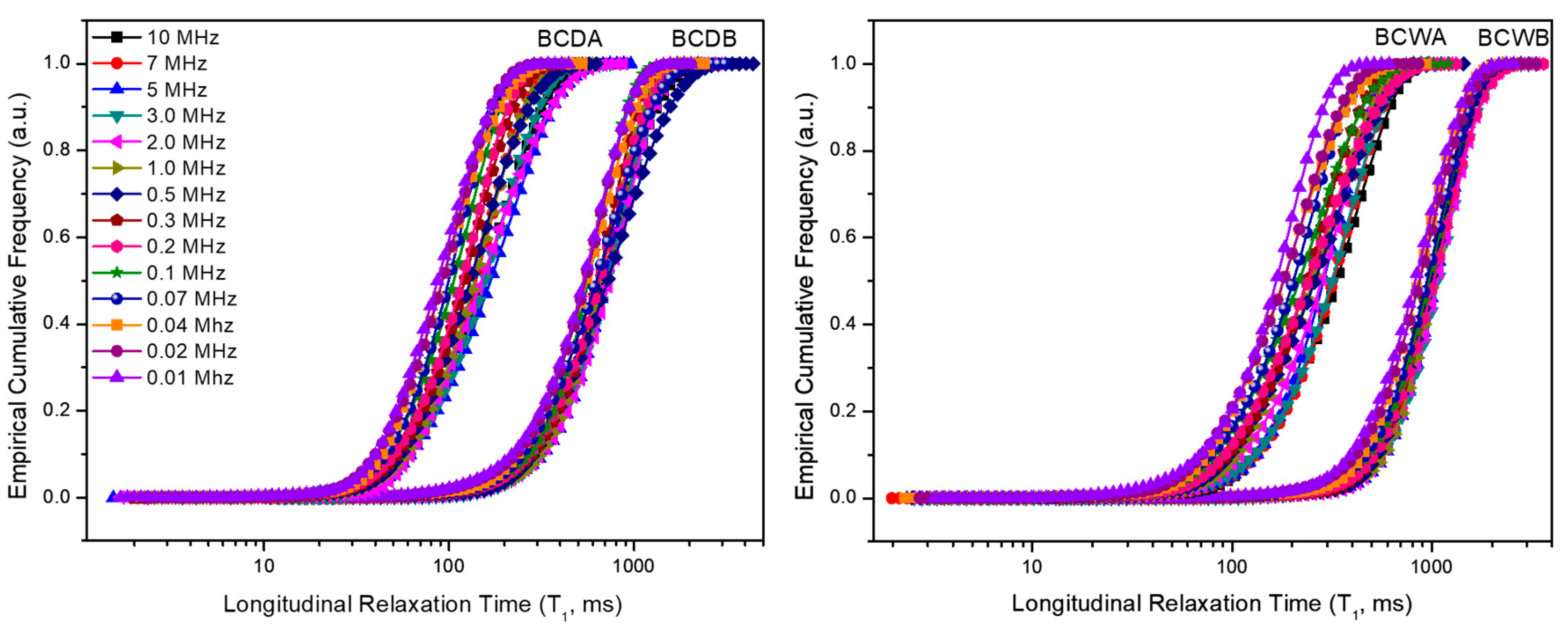
As previously mentioned, the inverse Laplace transform relaxograms describe distributions of longitudinal relaxation times that, in turn, are directly related to the pore size distribution of a porous material (assuming that the surface relaxivity is the same for all the surfaces). It is worth recalling here that the shorter the $T_1$ value, the more constrained the water molecules are as a consequence of their entrapment into micro-pores. As the $T_1$ value lengthens, water molecules move into pores that are progressively larger (e.g., meso- and macropores). The integration of the NMR relaxogram provides an S-shaped curve representing a non-exceeding empirical cumulative frequency $\mathsf{\Phi }\left(T_1\right)$, i.e., the longitudinal relaxation time assumes a value that is less than or equal to a given $T_1$ value.

Two different parts can be recognized in the $\mathsf{\Phi }\left(T_1\right)$ function. The first one is defined by the integral given in (5), where $A_{tot}$ is the total area of the relaxogram:

$$\mathsf{\Phi }\left(T_{\mathrm{A}}\right)=\frac{1}{A_{tot}}{{\displaystyle \int }}_0^{T_A}D\left(T_1\right)d{T}_1=0.01$$

(5)

This describes the zone corresponding to the shortest $T_1$ values within a time range referred to as $T_A$. Equation (5) means that only 1% of the measured relaxation times are less or equal to $T_A$ (fast relaxing component).

The second $\mathsf{\Phi }\left(T_1\right)$ part is given in the integral reported in (6), where $A_{tot}$ has the same meaning as before:

$$\mathsf{\Phi }\left(T_{\mathrm{B}}\right)=\frac{1}{A_{tot}}{{\displaystyle \int }}_0^{T_B}D\left(T_1\right)d{T}_1=0.99$$

(6)

It describes the zone associated with the longest longitudinal relaxation times, included in a range indicated as $T_B$. Equation (6) means that only 1% of the measured $T_1$ values are larger than or equal to $T_B$ (slow relaxing component).

According to Conte and Ferro [31,32,33], the solution of the integrals in (5) and (6) provides the parameters (i.e., $T_A$, and $T_B$) which can be applied to define two “connectivity indexes”. They are the Structural Connectivity Index (SCI) and the Functional Connectivity Index (FCI) calculated according to the following expressions:

$$SCI=CV\left(T_1\right)$$

(7)

$$FCI=T_B/T_A$$

(8)

in which $CV\left(T_1\right)$ is the coefficient of variation of the relaxation time $T_1$ values occurring in the range 0.01 < $\mathsf{\Phi }\left(T_1\right)$ < 0.99

The SCI represents the overall spatial organization of the soil particles leading to the formation of pores and channels where water molecules move. The FCI represents the ability of water exchange among different pores or particle aggregates mediated by the chemical–physical interactions with the pore boundaries.

2.7.2. The PCI Model

According to general theory, the longitudinal relaxation rate R₁ of a wet porous material depends on the different behavior of the water molecules either flowing in the pore lumen or interacting with the pore surface:

$$R_1=R_W+f_s\left(R_s-R_W\right)$$

(9)

where $R_W$ is the relaxation rate of bulk water, $f_s$ and $R_s$ are the mole fraction and the intrinsic relaxation rate for surface water, respectively. The assumption is that water molecules are continuously exchanged between the pore surface and the bulk. Thus:

$$f_s=\left(R_s-R_W\right)/\left(R_1-R_W\right)$$

(10)

In turn, $f_s$ can be related to the texture properties of the material through the relationships: $f_s=\lambda \left(m/D\right)$, and $f_s=\lambda \left(S/V\right)$, where $\lambda$ is the thickness of the hydration shell of the pore walls, $m$ is a geometry parameter (its value depends on the pore shape, i.e., m = 4 for cylindrical pores, 6 for spherical pores), $S$ and $V$ are the specific pore surface and volume, respectively, $D$ is the average pore diameter. The combination of the latter relationships leads to the following expressions, which can be found in literature:

$$R_1=R_W+\lambda \left(m/D\right)\left(R_s-R_W\right)$$

(11)

$$R_1=R_W+\rho \left(m/D\right)$$

(12)

$$R_1=R_W+\rho \left(S/V\right)$$

(13)

where $\rho$ is the so-called “surface relaxivity”.

By examining the actual relaxation kinetics of the sample, different conditions can be observed. Indeed, relaxation of different nuclei actually occurs at different rates, according to a frequency distribution, $D\left(T_1\right)$, given by the inverse Laplace transform of the kinetic data. Therefore, the relaxation kinetics should be actually expressed in an integral form as follows:

$$M\left(t\right)=M_{t=\infty }+\left(M_{t=0}-M_{t=\infty }\right){{\displaystyle \int }}_{T_1=0}^{\infty }D\left(T_1\right)e^{-t/T_1}d{T}_1$$

(14)

In the simplest case, this reduces to a relatively narrow unimodal Lognormal distribution, and, hence, the relaxation kinetics can be reasonably fitted as an ordinary first-order mono-exponential expression. In general, this is not the case, and the inverse Laplace transform instead consists of an asymmetric distribution, which frequently appears as the convolution of two (or more) partly superimposed contributions. Under these circumstances, in the case of wet systems, Conte and Ferro [31,32,33] proposed (see above) to define two suitable “connectivity indexes”, namely SCI and FCI, which are intended to quantify the functional transport properties of a solid porous system, such as soil.

A further interesting behavior can be observed for the wet nano sponges (i.e., hyper-reticulated cyclodextrin or calixarene polymers) which can be considered soft, porous materials. In fact, in this case, the distribution function $D\left(T_1\right)$ obtained from the inverse Laplace transform features a bimodal distribution with two distinct asymmetric Lognormal components, which can be attributed to the relaxometric behavior of (i) the free water molecules flowing within the pore network (“slow” relaxation component $D(T_{slow})$) and (ii) cumulatively to the surface water molecules and the skeletal hydrogen atoms of the organic framework (“fast” relaxation component $D(T_{fast})$). Under these circumstances, the relaxation kinetics follows a trend that can be suitably fitted as the sum of two independent exponential terms, from which two distinct relaxation rates $R_{1slow}$ and $R_{1fast}$ can be obtained. Hence, Lo Meo et al. [35] introduced PCI defined as follows:

$$PCI=\frac{{\left({{\displaystyle \int }}_{T_{A,fast}}^{T_{B,fast}}D\left(T_{fast}\right)T_{fast}d{T}_{fast}\right)}^{-1}-R_w}{{\left({{\displaystyle \int }}_{T_{A,slow}}^{T_{B,slow}}D\left(T_{slow}\right)T_{slow}d{T}_{slow}\right)}^{-1}-R_w}$$

(15)

where the integration limits are defined as follows:

$$\begin{gathered} {{\displaystyle \int }}_0^{T_{A,fast}}D\left(T_{fast}\right)d{T}_{fast}=0.025;{{\displaystyle \int }}_0^{T_{B,fast}}D\left(T_{fast}\right)d{T}_{fast}=0.975 \\ {{\displaystyle \int }}_0^{T_{A,slow}}D\left(T_{slow}\right)d{T}_{slow}=0.025;{{\displaystyle \int }}_0^{T_{B,slow}}D\left(T_{slow}\right)d{T}_{slow}=0.975 \end{gathered}$$

(16)

The same treatment can be applied, in principle, even in the case that the Φ(T₁) frequency distribution function can be reasonably subjected to deconvolution analysis into two distinct (though superimposed) distributions.

2.7.3. The Heuristic Algorithm

In whatever way the relaxation kinetics has to be treated, and the relevant relaxation rates $R_1$ as a function of the magnetic field are obtained, the problem arises of how the relevant NMRD dispersion curves have to be further analyzed in order to obtain the final information about the correlation times ${\tau }_c$ (i.e., the time needed for a molecule to rotate one radian or to move for a distance as long as its gyration diameter). By the way, in the case of the soft NS, for which two distinct rates (“slow” and “fast”) are obtained, two distinct NMRD curves have to be built as well. According to the well-known Bloembergen–Purcell–Pound (BPP) theory [36], for an ideal “simple” molecular system, subjected to a single dynamic regime, relaxation rates should depend on ${\tau }_c$ according to the relationship:

$$R_1=\frac{1}{T_1}=\frac{3}{10}\frac{{\mu }_0^2{\gamma }^4}{{\hslash }^2{r}^6}\left(\frac{{\tau }_c}{1+{\left({\omega }_L{\tau }_c\right)}^2}+\frac{4{\tau }_c}{1+4{\left({\omega }_L{\tau }_c\right)}^2}\right)$$

(17)

where $r$ is the internuclear distance, ${\omega }_L=2\pi {\nu }_L$ is the proton Larmor angular frequency (rad s⁻¹), $\gamma$ is the gyromagnetic ratio that is a constant for each NMR observable nucleus, $\hslash$ is the Dirac constant, and ${\mu }_0$ is the proton magnetic permeability. For complex systems, possibly made of different components subjected to different dynamics, one should derive, in principle, the correct expression based on the spectral density functions, which, in turn, derive from the autocorrelation function for the relaxing nuclei. Unfortunately, such a rigorous approach needs a robust mathematical elaboration. Alternatively, a “model-free” approach may provide a viable solution. The main conceptual issues involved in the model-free analysis have been particularly addressed in the seminal papers by Halle et al. [37], who proposed to adapt a generic NMRD curve as a sum of an adjustable number of Lorentzian functions:

$$R_1={(T_1)}^{-1}={{\displaystyle \sum }}_i\frac{c_i{\tau }_i}{1+{\left(\omega {\tau }_i\right)}^2}$$

(18)

Hence, the requested apparent correlation time $\langle {\tau }_c\rangle$ can be calculated as follows:

$$\langle {\tau }_c\rangle =\frac{{{\displaystyle \sum }}_i{C}_i{\tau }_c}{{{\displaystyle \sum }}_i{C}_i}$$

(19)

Subsequently, Kruk et al. [38] proposed to treat the NMRD curves of proteins as the sum of three terms:

$$R_1=R_0+R^{HH}+R^{NH}$$

(20)

where $R_0$ is an offset term accounting for very fast dynamic components (${\tau }_c<1 ns$), $R^{HH}$ describes the homonuclear relaxation as a sum of three BPP-like terms, and $R^{NH}$ is a complex ad hoc term to take into account the effect (i.e., the “quadrupolar peaks” in the NMRD profiles) of the quadrupolar interactions with nitrogen nuclei. In order to overcome the conceptual difficulties arising from the degree of discretionarily in the choice of Lorentzian or BPP components typical of model-free approaches, very recently Lo Meo et al. [34] proposed a heuristic analysis method, based on the assumption that, in principle, a complex system may be viewed as a continuum of virtual dynamic domains, each describable in terms of a BPP-like function with a proper ${\tau }_c$ value. Hence, the second term of Equation (18) can be transformed into an integral form:

$$R^{HH}={{\displaystyle \int }}_0^{\infty }\left[\left(\frac{{\tau }_c}{1+{\left(\omega {\tau }_c\right)}^2}+\frac{4{\tau }_c}{1+4{\left(\omega {\tau }_c\right)}^2}\right)\right]f^{*}\left({\tau }_c\right)d{\tau }_c$$

(21)

where a suitable distribution function $f^{*}\left({\tau }_c\right)$ is present, providing a complete description of the system dynamics, which constitutes the Inverse Integral Transform of the experimental NMRD curve, with the BPP function as the kernel. By applying this type of analysis to diverse systems (including NS, cellulose, and cheese), it unexpectedly turned out that the $f^{*}\left({\tau }_c\right)$ function features a limited number of sharp peaks, each pointing out at an individual dynamic domain, which in turn can be related to a particular physical–chemical characteristic of the system, without introducing any element of discretionarily in the analysis.

3. Results

3.1. The SCI-FCI Model

According to the elaboration described in Materials and Methods, the non-exceeding empirical cumulative frequency, $\mathsf{\Phi }\left(T_1\right)$, at different proton Larmor frequencies (${\nu }_L$) were obtained and examined.

Figure 1 reports $\mathsf{\Phi }\left(T_1\right)-\mathrm{vs}.-T_1$ for the four biochars under investigations. It appears that, prior to application to soil, the $\mathsf{\Phi }\left(T_1\right)$ curves at each ${\nu }_L$ for BCDB differed between each other for their limbs, whereas no (or only slight) differences were observed for BCWB.

The $\mathsf{\Phi }\left(T_1\right)$ curves acquired for the biochars collected after seven weeks from the application to soil (BCDA, and BCWA, respectively) were not only shifted towards shorter $T_1$ values, but also showed large differences in their limbs.

A visual inspection of the $\mathsf{\Phi }\left(T_1\right)$ curves in Figure 1 reveals that all the high components (i.e., the longest $T_1$ values) were shorter than the low components (i.e., the shortest $T_1$ values). According to Conte and Ferro [31,32,33], this means that the SCI values were always smaller than the FCI ones. Moreover, according to the data treatment reported in the literature [31,32,33], the measured FCI and SCI values were normally distributed (Figure 2). For this reason, the FCI and SCI average values reported in the histograms of Figure 3 can be considered representative of the two measured parameters for any applied magnetic field.

Figure 3 shows that an increase in the FCI value could be observed in both biochars after their application to soil. An analogous increase was observed for the wet−quenched biochar SCI (BCWB-vs.-BCWA), whereas no changes were observed for the SCI value of the dry−quenched biochar (BCDB-vs.-BCDA).

3.2. The PCI Model

The Pore Connectivity Indexes (PCI) for the four samples analyzed here were obtained as reported in Materials and Methods either by using the decay/recovery curves reported in Figure A1 (Appendix A) or the relaxograms shown in Figure A2 (Appendix B). Regardless of the input data-set used for the PCI achievement at different ${\nu }_L$ values, all the PCIs appeared normally distributed (Figure 4).

Thus, two sets of mean PCI values were obtained. The first one was achieved by averaging the data calculated by using the decay/recovery curves at each ${\nu }_L$ (Figure 5A), while the second one was retrieved by the average of the PCI values calculated from the relaxograms obtained by the UPEN algorithm (Figure 5B).

Figure 5 shows that, regardless of the data set used to obtain the PCI values, a decrease was observed for biochars (i.e., the dry−quenched and the wet−quenched ones) after application to soil.

3.3. The Heuristic Algorithm

The NMRD profiles of the four biochars studied herein are reported in Figure 6. It can be noted that before the application to soil, the dry−quenched biochar (BCDB) relaxed faster than the wet−quenched one (BCWB) in the whole range of the applied magnetic fields. The same trend was observed for the biochars after application to soil (BCDA and BCWA, respectively). Moreover, the NMRD curves of both biochars after soil application showed faster longitudinal relaxation rates as compared to the curves acquired for the biochar prior to their use. The fitting curves (continuous lines) in Figure 6 were obtained by applying the heuristic method described in Materials and Methods. All coefficients of correlation (R²) were larger than 0.98, outlining the good fitting ability of the algorithm.

As an additional result from the application of the heuristic algorithm, the obtained correlation time spectra are reported in Figure 7. With the exception of the sample BCDB, all the biochars revealed that the water molecules in equilibrium with the solid surfaces were characterized by three different correlation times. This means that at least three types of molecules with different dynamic regimes could be identified in BCDA, BCWB, and BCWA when they were suspended in Milli-Q grade water, as indicated in Materials and Methods.

4. Discussion

4.1. Chemical Characteristics of the Biochars as Affected by the Quenching Procedure

As already discussed in the Materials and Methods section, biochars were produced by using the same feedstock and stove via the application of two different quenching procedures. On the one hand, pyrolysis was terminated simply by switching off the energy supply and letting the system cool to room temperature (sample BCDB). On the other hand, cool water was added to the system, and the thermal degradation was abruptly interrupted (sample BCWB). The two quenching procedures allowed obtaining biochars with different chemical characteristics. Indeed, the elemental analyses revealed that BCDB had a 76.0 ± 0.5% C content and 0.29 ± 0.03% N content, whereas BCWB had a 58 ± 3% C content and a 0.24 ± 0.02% N content. The larger amount of carbon in BCDB, as compared to BCWB, can be only explained by considering the different quenching rates of the two pyrolysis procedures. In fact, the dry−quenching procedure allowed a longer period of time for the pyrolyzed biomass to cool to room temperature as compared to the period of time needed by the quenching procedure with water. Consequently, the thermal degradation of the biomass continued even after the energy supply was turned off. Therefore, all the organic components present in the fir-wood pellets were reduced to polyaromatic systems, as described in Conte et al. [1] and Rafiq et al. [39]. Conversely, when the pyrolysis was quenched with water, the cooling of the system was much quicker. Therefore, organic components, such as carbohydrates and proteins, in the fir-wood pellets were partly preserved, thereby making the resulting biochar more hydrophilic (with a larger oxygen content) than the dry−quenched one. The comparable amount of nitrogen in the two biochars reflects the nature of the feedstock, which, as aforementioned, was made by fir-wood pellets. However, according to the discussion above, it is possible to hypothesize that most of the nitrogen in BCDB was in heterocyclic aromatic systems (HAS), whereas it was only partly in the form of HAS in BCWB, was also preserved in N-containing structures usually present in plant tissues (e.g., proteins, DNA, and so on).

The different cooling rates responsible for the diverse C content in BCDB and BCWB also affected the BET surface areas (SA), which were in the order SA_BCDB > SA_BCWB. As indicated by Conte et al. [1], the longer the pyrolysis temperature is maintained, the larger is the surface area of the produced biochar. Therefore, since the fir-wood pellets were practically kept at high temperatures for a longer time during the dry−quenching procedure, the resulting BCDB had a surface area larger than that measured for BCWB. Further confirmation about the extent of thermal degradation in the dry−quenching procedure came from the evaluation of the biochar pH values. Namely, they were 9.44 ± 0.02 for BCDB and 9.00 ± 0.04 BCWB. This trend accords with Rafiq et al.’s [39] results for similar cases.

Due to the use of water as a cooling material for the pyrolysis quenching, the amount of residual water in BCWB was sensibly larger than in BCDB. Indeed, it was 1.13 ± 0.04% for the latter and 32.5 ± 0.4% for the former biochar. It is very likely that such a significant amount of water clogs the BCWB pore system, thereby making it less available for the penetration of the Milli-Q water used in the FFC NMR relaxometry experiments (see below).

4.2. Biochar Characteristics by the SCI-FCI Model

Figure 1 reports the empirical cumulative frequency distribution curves for the four different biochars studied here. As evidenced, the $\mathsf{\Phi }\left(T_1\right)$ curves for BCDA and BCWA shifted to the left-hand side of the BCDB and BCWB ones. According to Conte and Ferro [32], this means that soil application produced a material (namely, BCDA and BCWA) with a pore system made by smaller pores as compared to the fresh biochars from the dry− and wet−quenching procedures (i.e., BCDB and BCWB). Indeed, as pore size reduces, the motion of water molecules is constrained due to stronger interactions with the wall of the pore boundaries [28]. Conversely, in larger-sized pores, water can move more freely and unconstrained [28]. Therefore, a first general conclusion provided by the qualitative evaluation of Figure 1 may be that, after application to soil, the parent biochars (i.e., BCDB, and BCWB) were physically transformed, thereby producing two materials (i.e., BCDA, and BCWA) having a pore system very different than the one present in the parent ones. However, it must also be highlighted that strong interactions between water molecules and porous systems’ surfaces can also be due to a larger number of surficial H-bond acceptors coming from biochar surface oxidation [21]. In other words, the simple eye evaluation of Figure 1 is not conclusive about the mechanisms involved in the biochar–water surface interactions.

FCI, i.e., the functional connectivity index, measures the ability of water exchange among different pores mediated by the chemical–physical interactions with the pore boundaries. SCI, i.e., the structural connectivity index, is a measure of the overall spatial organization of the particles of a porous system leading to the formation of pores and channels [31,32,33]. Figure 3 shows that FCI increased after the biochar was applied to the soil. As a consequence, it is possible to hypothesize that the motion of the water molecules in contact with the surfaces of BCDA and BCWA was reduced due to the formation of a number of surficial H-bonds higher than those forming on the surfaces of BCDB and BCWB. The increase in the number of surficial interactions can be explained by considering that biochar was subjected to rapid oxidation when placed into soil [21]. Therefore, the larger number of oxygenated functions consequent to oxidation provided more surficial sites to which water molecules can be hooked. Noteworthy, SCI values revealed different trends for the dry– and wet–quenched biochars, respectively (Figure 3). Indeed, no differences were visible for BCDB and BCDA, whereas the SCI increase was measurable after BCWB was applied to soil (Figure 3). The increase in SCI values was due to the physical alteration of the porous–system particles. In particular, following Conte and Ferro [33], it seems that the finding of BCWA having the highest SCI value can be explained by the presence of larger pores as compared to the BCWB sample. The interpretation of data coming from the qualitative evaluation of Figure 1 and the quantitative assessment of the FCI and SCI values given in Figure 3 suggests that when the biochar from the dry−quenched procedure was placed into soil, no (or very limited, i.e., not measurable by the SCI-FCI model) physical alterations occurred (that is, no SCI variations going from BCDB to BCDA). Conceivably, the surface of the dry–quenched biochar was predominantly subjected to oxidation with the formation of oxidated surficial sites [21] that can hook water molecules, thereby inhibiting their motion (increase in FCI values).

When the wet–quenched biochar was placed into soil, both physical alterations and surface chemical oxidation occurred. In particular, the physical alterations may consist of a structural rearrangement that produces a more complex net of channels and pores (increase in SCI value going from BCWB to BCWA) [33]. Concomitantly, surface oxidation [21] allowed the formation of oxygenated “arms” not only on the biochar surface but also on the walls of channels and pores. The aforementioned “arms” can interact with water molecules, thus retaining them inside and around the whole biochar system.

In order to understand why BCWA was made by a more complex net of channels and pores as compared to BCWB, it must be reminded that, due to the wet quenching, the water content in the BCWB was 32.5 ± 0.4% (see above). For this reason, as this biochar was placed into soil, the water occluded in the BCWB pore system was released, thereby producing the aforementioned structure alterations.

4.3. Biochar Characteristics by the PCI Model

Figure 5 reports the PCI values obtained by applying the PCI model to the decay/recovery curves (Figure 5A) and the relaxograms (Figure 5B). In both cases, a PCI decrease was observed. The differences among the absolute values reported in Figure 5A,B can be attributed to the different PCI model “sensitivity” when it was applied on the decay/recovery curves or the relaxograms. Indeed, the decay/recovery curves can be considered as the original raw data. They came directly from the NMR machine, while the relaxograms originated by manipulating the raw data via the inverse Laplace transformation with the UPEN algorithm. For this reason, the former can be more reliable than the latter. However, more experiments are needed to confirm such a hypothesis.

According to Lo Meo et al. [35], PCI is related to the water motion in reticulated soft systems (e.g., nano sponges) as affected by the strength of the interactions between water and the walls of the reticules. As the reticulation degree increases, a decrease in the pore connectivity index is observed as a consequence of the more intimate contact between water and the soft reticulated system. In the case of the samples studied here, the PCI decrease can be explained by considering that, after application to soil, the biochars were subjected to physical and chemical alterations. The physical alterations were more evident for BCWB transformed in BCWA than BCDB going to BCDA. When both BCDB and BCWB were placed into the soil, their water content was released. However, BCDB water content was smaller than that of BCWB. Therefore, after soil application, BCWB was transformed to BCWA with a reticulation degree (i.e., the net of channels and pores) more complex than that belonging to BCDA obtained by the transformation of BCDB. Due to the concomitant surface oxidation [21], water molecules were more effectively retained in the biochars after soil application.

4.4. The Heuristic Algorithm

Figure 6 shows the NMRD profiles of the water suspended biochars analyzed in the present study.

NMRD profiles report the longitudinal relaxation rates of the observed nuclei (e.g., protons) versus the proton Larmor frequency. The profiles reflect molecular dynamics of the components of complex systems and provide important information about the motion of water and nutrients in environmentally relevant porous systems (e.g., soils and biochars). In the present study, the experimental longitudinal relaxation rates were fitted to Equation (20) by applying the heuristic algorithm. The continuous lines represented the model fit of each biochar sample.

The NMRD profile acquired for BCDB was placed at $R_1$ values faster than those revealed for BCWB in the whole range of proton Larmor frequencies used here. This can be explained by considering the different numbers of water molecules clogging the pore systems of the two biochars. As outlined above, the water content in BCDB was 1.13 ± 0.04%, while it was 32.5 ± 0.4% in BCWB. Due to this, it is conceivable that the BCDB pore system was more accessible to the Milli-Q grade water used for the FFC NMR experiments than the water–clogged pore system in BCWB. The different pore accessibility made it possible for water to be more constrained in BCDB than in BCWB. In fact, the slower the motion, the faster the $R_1$ value is. Conversely, when the motion is unconstrained, the longitudinal relaxation rate slows down [28]. Finally, as a consequence of the physical and chemical transformations described above, the two BCDA and BCWA biochars entrapped water molecules better than BCDB and BCWB.

The relative position of the BCDA and BCWA NMRD profiles can be explained by the different pore distributions in the two samples. Namely, BCDA can be characterized by a larger porosity than BCWA.

The application of the heuristic algorithm on the NMRD profiles produced the fitting curves reported in Figure 6 and the distribution of correlation times shown in Figure 7. In particular, BCDB revealed two different types of water molecules. One could be associated with very constrained water (${\tau }_C=1.7 \mathsf{\mu }\mathrm{s}$), while the second was associated with more unconstrained water molecules (${\tau }_C=11\mathsf{\mu }\mathrm{s}$). After application to soil, three different types of water molecules could be identified in BCDA: ${\tau }_C=0.63 \mathsf{\mu }\mathrm{s}$, ${\tau }_C=4.5 \mathsf{\mu }\mathrm{s}$, and ${\tau }_C=28 \mathsf{\mu }\mathrm{s}$ (Figure 7). It is evident that the shortest correlation time in BCDB (${\tau }_C=1.7 \mathsf{\mu }\mathrm{s}$) became smaller in BCDA (${\tau }_C=0.63 \mathsf{\mu }\mathrm{s}$). The same can be observed for the second correlation time, going from 11 $\mathsf{\mu }\mathrm{s}$ in BCDB to 4.5 $\mathsf{\mu }\mathrm{s}$ in BCDA. The shortening of correlation times can be explained by the higher BCDB hydrophobicity as compared to BCDA. Because of the larger hydrophobicity, water molecules around BCDB were clustered. In other words, they tended to form stronger H-bonds between each other in order to compensate for the biochar surface hydrophobicity. The formation of the clusters makes water molecules “rigid”, thereby providing the aforementioned BCDB correlation times.

After soil application, the biochar surface becomes more hydrophilic due to oxidation [21]. Therefore, water molecules in the clusters become more flexible, and shorter correlation times are measured.

The surface oxidation also allowed the achievement of the third type of water molecules showing a correlation time of 28 $\mathsf{\mu }\mathrm{s}$ (Figure 7). These were water molecules directly bound to the oxygenated surficial sites.

The water suspended BCWB sample revealed three correlation times: ${\tau }_C=1.3 \mathsf{\mu }\mathrm{s}$, ${\tau }_C=7.9 \mathsf{\mu }\mathrm{s}$, and ${\tau }_C=158 \mathsf{\mu }\mathrm{s}$. The first two correlation times have the same meaning as for BCDB. They describe the behavior of water molecules in the hydration sphere around biochar. Due to the wet−quenching procedure, the third correlation time of 158 mu s was due to the Milli-Q grade water molecules strongly interacting with those trapped in the BCWB pore system.

Following the application to soil and surface oxidation [21], BCWA surface can be considered more hydrophilic than that of BCWB. Therefore, a reduction in the correlation time could be observed for the water molecules inside the hydration sphere. Noteworthy, a reduction in the third ${\tau }_C$ value from 158 to 112 $\mathsf{\mu }\mathrm{s}$ was also observed. A plausible explanation for this reduction could be that the Milli-Q grade water was not anymore bound to the water molecules clogging the pore system (as they have been released into the soil) but to the oxygenated surficial sites. H-bonds are stronger when they form between water molecules rather than when they are unconventional as described in Conte et al. [23]. As a consequence, they were more flexible in BCWA than in BCWB.

5. Conclusions

The present study was aimed at understanding the physicochemical alterations of biochar when it was applied to the soil. In particular, fir wood pellets were used to produce dry–quenched and wet–quenched biochar. The two types of biochar produced by the two different procedures were subjected to different mechanisms of alteration when placed into the same soil. In fact, while the dry–quenched biochar was mainly chemically modified, that obtained by the wet–quenching procedure was both physically and chemically altered. In other words, the dry−quenching produced a material that mainly underwent surficial oxidization, while its porosity was almost unchanged. Conversely, the porosity degree and surficial chemistry of the biochar produced by the wet–quenching procedure were modified when it was incorporated into the soil. Due to these diverse transformations, the dry– and wet–quenched biochars revealed different attitudes to retaining water. From a practical point of view, the results of the present study suggest that the biochar production procedure can be changed according to the use of the biochar one intends to implement to solve specific soil problems. As an example, we can expect that the application of the dry–quenched biochar may result in a better crop yield as compared to the soil treated with the wet–quenched material. In fact, due to its higher hydrophilic character following aging in soil, the dry−quenched biochar may promote higher water retention, hence, reduced nutrient leaching and higher crop yield. Conversely, the wet–quenched biochar became more hydrophobic because of the aging in soil. Therefore, it may allow water and nutrient leaching towards the deeper horizons of the soil profile and a reduction in plant growth. Inferences can, therefore, be drawn from these observations when biochar is applied for soil remediation purposes. In fact, it can be expected that the higher hydrophilicity of BCDA may allow better contaminant retention on the soil surface, thus preventing leaching towards groundwaters.

In the present study, a number of different mathematical models to interpret relaxometric data were used. In particular, a model (referred to as SCI-FCI) used for the analyses of soils (i.e., hard matter) was compared to that (referred to as PCI) developed for the investigation of nano sponges (i.e., soft matter). With a different grade of sensitivity, both mathematical models provided the same answers, thereby revealing that they can also be applied to biochar that can be considered a material with physical properties intermediate between hard and soft systems. Moreover, the results reported in the present study suggest also that the SCI-FCI and the PCI models can be joined together for the elaboration of a unified model. The latter could have more general applicability than the two single ones being usable on any kind of material. However, this is the aim of an ongoing study from our research group. The present study also revealed the suitability of the heuristic algorithm for the evaluation of the water behavior in biochar. In particular, it was possible to differentiate between water molecules in hydration spheres and those directly bound to the biochar surface.

References

1. Conte, P.; Bertani, R.; Sgarbossa, P.; Bambina, P.; Schmidt, H.; Raga, R.; Lo Papa, G.; Chillura Martino, D.F.; Lo Meo, P. Recent Developments in Understanding Biochar’s Physical–Chemistry. Agronomy 2021, 11, 615. [Google Scholar] [CrossRef]
2. European Biochar Foundation Guidelines for a Sustainable Production of Biochar. Available online: https://www.european-biochar.org/biochar/media/doc/ebc-guidelines.pdf (accessed on 6 July 2020).
3. Conte, P.; Schmidt, H.-P.; Cimò, G. Research and Application of Biochar in Europe. In Agricultural and Environmental Applications of Biochar: Advances and Barriers; Guo, M., He, Z., Uchimiya, S.M., Eds.; Soil Science Society of America, Inc.: Madison, WI, USA, 2015; pp. 409–422. ISBN 9780891189640. [Google Scholar]
4. Schmidt, H.-P.; Wilson, K. The 55 Uses of Biochar. Available online: https://www.biochar-journal.org/en/ct/2 (accessed on 15 June 2020).
5. Baiamonte, G.; De Pasquale, C.; Marsala, V.; Cimò, G.; Alonzo, G.; Crescimanno, G.; Conte, P. Structure alteration of a sandy-clay soil by biochar amendments. J. Soils Sediments 2015, 15, 816–824. [Google Scholar] [CrossRef]
6. Schmidt, H.; Pandit, B.; Martinsen, V.; Cornelissen, G.; Conte, P.; Kammann, C. Fourfold Increase in Pumpkin Yield in Response to Low-Dosage Root Zone Application of Urine-Enhanced Biochar to a Fertile Tropical Soil. Agriculture 2015, 5, 723–741. [Google Scholar] [CrossRef] [Green Version]
7. Nicosia, A.; Pampalone, V.; Ferro, V. Effects of Biochar Addition on Rill Flow Resistance. Water 2021, 13, 3036. [Google Scholar] [CrossRef]
8. Alkharabsheh, H.M.; Seleiman, M.F.; Battaglia, M.L.; Shami, A.; Jalal, R.S.; Alhammad, B.A.; Almutairi, K.F.; Al-Saif, A.M. Biochar and its broad impacts in soil quality and fertility, nutrient leaching and crop productivity: A review. Agronomy 2021, 11, 993. [Google Scholar] [CrossRef]
9. Kammann, C.I.; Schmidt, H.-P.; Messerschmidt, N.; Linsel, S.; Steffens, D.; Müller, C.; Koyro, H.-W.; Conte, P.; Stephen, J. Plant growth improvement mediated by nitrate capture in co-composted biochar. Sci. Rep. 2015, 5. [Google Scholar] [CrossRef]
10. Gwenzi, W.; Chaukura, N.; Noubactep, C.; Mukome, F.N.D. Biochar-based water treatment systems as a potential low-cost and sustainable technology for clean water provision. J. Environ. Manag. 2017, 197, 732–749. [Google Scholar] [CrossRef]
11. Rao, M.A.; Di Rauso Simeone, G.; Scelza, R.; Conte, P. Biochar based remediation of water and soil contaminated by phenanthrene and pentachlorophenol. Chemosphere 2017, 186. [Google Scholar] [CrossRef]
12. Li, X.; Wang, C.; Zhang, J.; Liu, J.; Liu, B.; Chen, G. Preparation and application of magnetic biochar in water treatment: A critical review. Sci. Total Environ. 2020, 711, 134847. [Google Scholar] [CrossRef]
13. da Silva Veiga, P.A.; Schultz, J.; da Silva Matos, T.T.; Fornari, M.R.; Costa, T.G.; Meurer, L.; Mangrich, A.S. Production of high-performance biochar using a simple and low-cost method: Optimization of pyrolysis parameters and evaluation for water treatment. J. Anal. Appl. Pyrolysis 2020, 148, 104823. [Google Scholar] [CrossRef]
14. Gwenzi, W.; Chaukura, N.; Wenga, T.; Mtisi, M. Biochars as media for air pollution control systems: Contaminant removal, applications and future research directions. Sci. Total Environ. 2021, 753, 142249. [Google Scholar] [CrossRef] [PubMed]
15. Smith, P. Soil carbon sequestration and biochar as negative emission technologies. Glob. Chang. Biol. 2016, 22, 1315–1324. [Google Scholar] [CrossRef] [PubMed]
16. Zhang, C.; Zeng, G.; Huang, D.; Lai, C.; Chen, M.; Cheng, M.; Tang, W.; Tang, L.; Dong, H.; Huang, B.; et al. Biochar for environmental management: Mitigating greenhouse gas emissions, contaminant treatment, and potential negative impacts. Chem. Eng. J. 2019, 373, 902–922. [Google Scholar] [CrossRef]
17. Jeffery, S.; Verheijen, F.G.A.; van der Velde, M.; Bastos, A.C. A quantitative review of the effects of biochar application to soils on crop productivity using meta-analysis. Agric. Ecosyst. Environ. 2011, 144, 175–187. [Google Scholar] [CrossRef]
18. Xu, G.; Zhang, Y.; Sun, J.; Shao, H. Negative interactive effects between biochar and phosphorus fertilization on phosphorus availability and plant yield in saline sodic soil. Sci. Total Environ. 2016, 568, 910–915. [Google Scholar] [CrossRef]
19. Gonzaga, M.I.S.; Mackowiak, C.; de Almeida, A.Q.; de Carvalho Junior, J.I.T.; Andrade, K.R. Positive and negative effects of biochar from coconut husks, orange bagasse and pine wood chips on maize (Zea mays L.) growth and nutrition. Catena 2018, 162, 414–420. [Google Scholar] [CrossRef]
20. Conte, P. Applications of Fast Field Cycling NMR Relaxometry. In Annual Reports on NMR Spectroscopy; Webb, G.A., Ed.; Academic Press—Elsevier: London, UK, 2021; pp. 141–188. ISBN 978-0-12-824620-7. [Google Scholar]
21. Hammes, K.; Schmidt, M.W.I. Changes of Biochar in Soil. In Biochar for Environmental Management; Lehmann, J., Joseph, S., Eds.; Earthscan Publisher: London, UK, 2009; pp. 169–181. [Google Scholar]
22. de Pasquale, C.; Marsala, V.; Berns, A.E.; Valagussa, M.; Pozzi, A.; Alonzo, G.; Conte, P. Fast field cycling NMR relaxometry characterization of biochars obtained from an industrial thermochemical process. J. Soils Sediments 2012, 12. [Google Scholar] [CrossRef]
23. Conte, P.; Marsala, V.; De Pasquale, C.; Bubici, S.; Valagussa, M.; Pozzi, A.; Alonzo, G. Nature of water-biochar interface interactions. GCB Bioenergy 2013, 5. [Google Scholar] [CrossRef] [Green Version]
24. Caporale, A.G.; Pigna, M.; Sommella, A.; Conte, P. Effect of pruning-derived biochar on heavy metals removal and water dynamics. Biol. Fertil. Soils 2014, 50. [Google Scholar] [CrossRef] [Green Version]
25. Bubici, S.; Korb, J.-P.; Kučerik, J.; Conte, P. Evaluation of the surface affinity of water in three biochars using fast field cycling NMR relaxometry. Magn. Reson. Chem. 2016, 54, 365–370. [Google Scholar] [CrossRef] [Green Version]
26. Conte, P.; Laudicina, V.A. Mechanisms of organic coating on the surface of a poplar biochar. Curr. Org. Chem. 2017, 21. [Google Scholar] [CrossRef] [Green Version]
27. Wilson, K.; Reed, D. IBI White Paper Implications and Risks of Potential Dioxin Presence in Biochar. Available online: https://www.biochar-international.org/wp-content/uploads/2018/04/IBI_White_Paper-Implications_of_Potential_ Dioxin_in_Biochar.pdf (accessed on 15 June 2020).
28. Conte, P. Environmental Applications of Fast Field-cycling NMR Relaxometry. In Field-cycling NMR Relaxometry: Instrumentation, Model Theories and Applications; Kimmich, R., Ed.; The Royal Society of Chemistry: Croydon, UK, 2019; pp. 229–254. ISBN 9781788011549. [Google Scholar]
29. Conte, P.; Lo Meo, P. Nuclear Magnetic Resonance with Fast Field-Cycling Setup: A Valid Tool for Soil Quality Investigation. Agronomy 2020, 10, 1040. [Google Scholar] [CrossRef]
30. Conte, P.; Di Stefano, C.; Ferro, V.; Laudicina, V.A.; Palazzolo, E. Assessing hydrological connectivity inside a soil by fast-field-cycling nuclear magnetic resonance relaxometry and its link to sediment delivery processes. Environ. Earth Sci. 2017, 76. [Google Scholar] [CrossRef]
31. Conte, P.; Ferro, V. Measuring hydrological connectivity inside a soil by low field nuclear magnetic resonance relaxometry. Hydrol. Process. 2018, 32. [Google Scholar] [CrossRef]
32. Conte, P.; Ferro, V. Standardizing the use of fast-field cycling NMR relaxometry for measuring hydrological connectivity inside the soil. Magn. Reson. Chem. 2020, 58, 41–50. [Google Scholar] [CrossRef]
33. Conte, P.; Ferro, V. Measuring hydrological connectivity inside soils with different texture by fast field cycling nuclear magnetic resonance relaxometry. Catena 2022, 209, 105848. [Google Scholar] [CrossRef]
34. Lo Meo, P.; Terranova, S.; Di Vincenzo, A.; Chillura Martino, D.; Conte, P. Heuristic Algorithm for the Analysis of Fast Field Cycling (FFC) NMR Dispersion Curves. Anal. Chem. 2021, 93, 8553–8558. [Google Scholar] [CrossRef]
35. Lo Meo, P.; Mundo, F.; Terranova, S.; Conte, P.; Chillura Martino, D. Water Dynamics at the Solid-Liquid Interface to Unveil the Textural Features of Synthetic Nanosponges. J. Phys. Chem. B 2020, 124, 1847–1857. [Google Scholar] [CrossRef]
36. Bloembergen, N.; Purcell, E.M.; Pound, R.V. Relaxation effects in nuclear magnetic resonance absorption. Phys. Rev. 1948, 73, 679–712. [Google Scholar] [CrossRef]
37. Halle, B.; Jóhannesson, H.; Venu, K. Model-Free Analysis of Stretched Relaxation Dispersions. J. Magn. Reson. 1998, 135, 1–13. [Google Scholar] [CrossRef] [Green Version]
38. Kruk, D.; Masiewicz, E.; Borkowska, A.M.; Rochowski, P.; Fries, P.H.; Broche, L.M.; Lurie, D.J. Dynamics of solid proteins by means of nuclear magnetic resonance relaxometry. Biomolecules 2019, 9, 652. [Google Scholar] [CrossRef] [PubMed] [Green Version]
39. Rafiq, M.K.; Bachmann, R.T.; Rafiq, M.T.; Shang, Z.; Joseph, S.; Long, R.L. Influence of pyrolysis temperature on physico-chemical properties of corn stover (zea mays l.) biochar and feasibility for carbon capture and energy balance. PLoS ONE 2016, 11, e0156894. [Google Scholar] [CrossRef] [Green Version]
Figure 1. The empirical cumulative frequency distribution curves at all the proton Larmor frequencies used in this study are plotted versus the longitudinal relaxation time ( T 1 ). BCDB, BCDA, BCWB, and BCWA stand for biochar (BC) dry—(D), and wet—(W) quenched, before (B), and after (A) application to soil.
Agriculture 12 00320 g001
Figure 2. The empirical cumulative frequency distribution for both FCI (A) and SCI (B) acquired at different proton Larmor frequencies (points) reveals a normal distribution shape (continuous lines). Hence, it can be suggested that the FCI and SCI values at each ν L can be averaged to obtain FCI and SCI mean values and standard deviations. The coefficients of determination reported in the figure were obtained by fitting the points with the normal distribution equation. In the legends, BC stands for biochar, D and W stand for dry−quench and wet−quench, respectively, B and A stand for before and after application to soil.
Agriculture 12 00320 g002
Figure 3. Mean and standard deviation values of Functional Connectivity Index (FCI) and Structural Connectivity Index (SCI). The values were obtained by averaging the FCI and SCI values at each ν L . The acronyms on the horizontal axes must be interpreted as it follows: BC stands for biochar, D and W lay for dry−quench and wet−quench, respectively, B and A stand for before and after application to soil.
Agriculture 12 00320 g003
Figure 4. The empirical cumulative frequency distribution for the PCI values obtained by the decay/recovery curves (A) and the UPEN algorithm (B) at each proton Larmor frequency (points) revealed a normal distribution shape (continuous lines). Hence, the mean and the standard deviation for the PCI values could be obtained by averaging all the values retrieved at each ν L either by the decay/recovery curves or by the UPEN algorithm. The coefficients of determination reported in the figure were obtained by fitting the points with the normal distribution equation. In the legends, BC stands for biochar, D and W stand for dry−quench and wet−quench, respectively, B and A stand for before and after application to soil.
Agriculture 12 00320 g004
Figure 5. Mean and standard deviation values of the Pore Connectivity Index (PCI) obtained from the decay/recovery curves (A) and UPEN algorithm (B). The values were obtained by averaging the PCI values at each ν L . The acronyms on the horizontal axes must be interpreted as follows: BC stands for biochar, D and W stand for dry−quench and wet−quench, respectively, B and A stand for before and after application to soil.
Agriculture 12 00320 g005
Figure 6. NMRD profiles of the four biochars studied here. The continuous lines were obtained by fitting the experimental data with the heuristic algorithm. In the legend, BC stands for biochar, D and W stand for dry−quench and wet−quench, respectively, B and A stand for before and after application to soil.
Agriculture 12 00320 g006
Figure 7. Correlation time distributions for the four biochars studied here.
Agriculture 12 00320 g007
Publisher’s Note: MDPI stays neutral with regard to jurisdictional claims in published maps and institutional affiliations.