
Prediction Model and Influencing Factors of CO2 Micro/Nanobubble Release Based on ARIMA-BPNN

Abstract
:1. Introduction
2. Materials and Methods
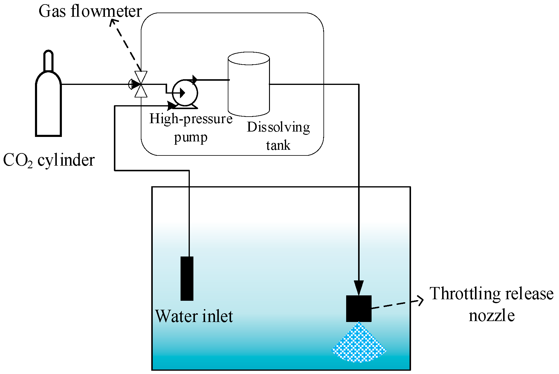
2.1. Preparation of CO2 Micro/Nanobubble Water
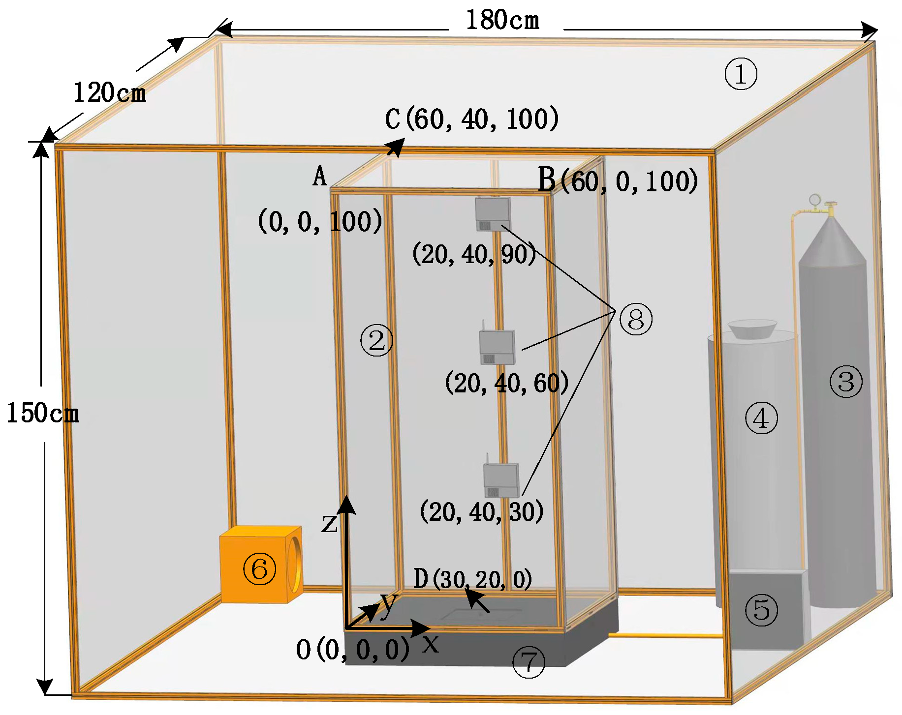
2.2. Construction of Experimental Environment
2.3. Design of CO2 Gas-Release Experiment
2.4. Data Analysis Tools
3. Fundamentals Analysis
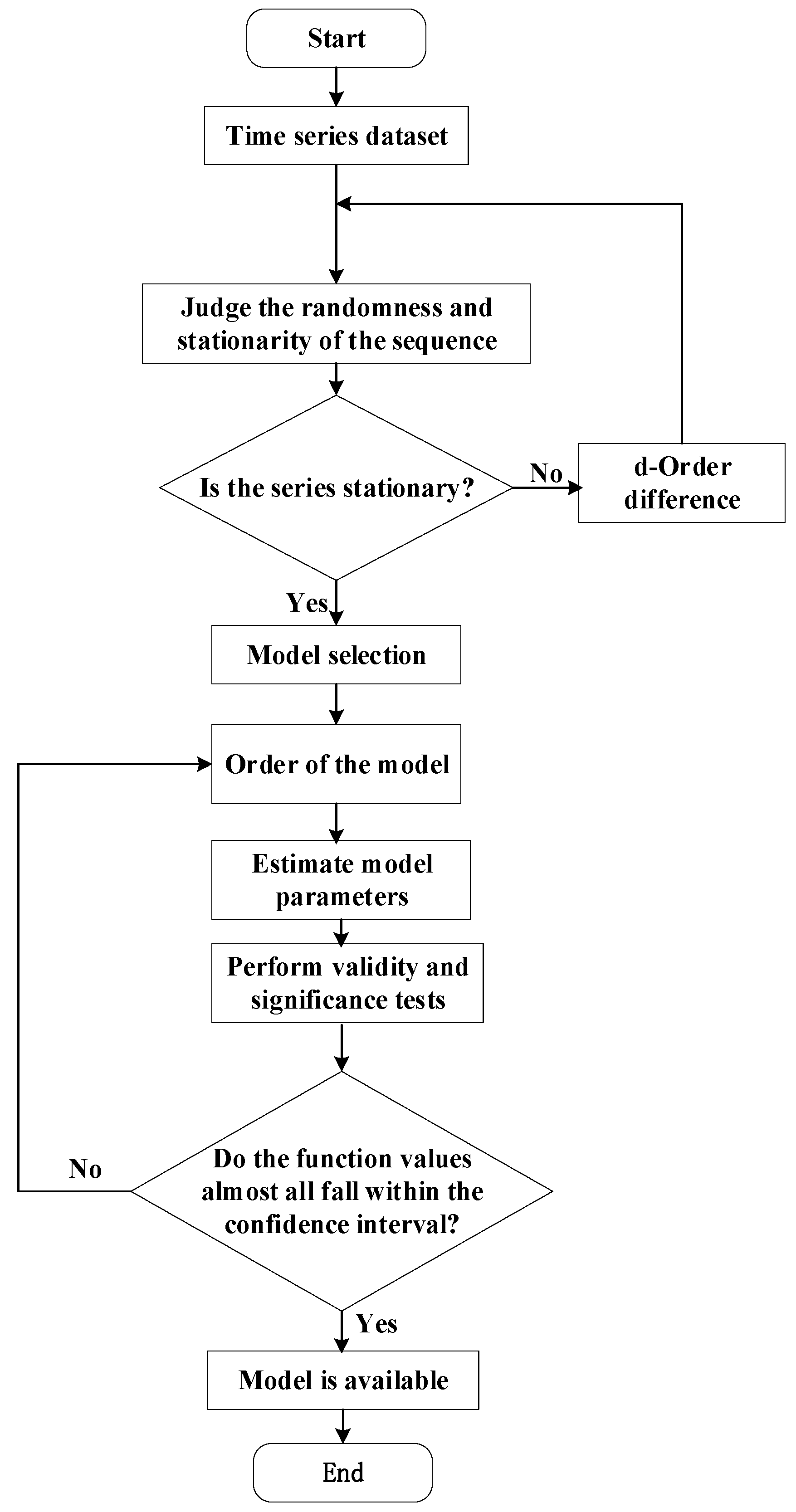
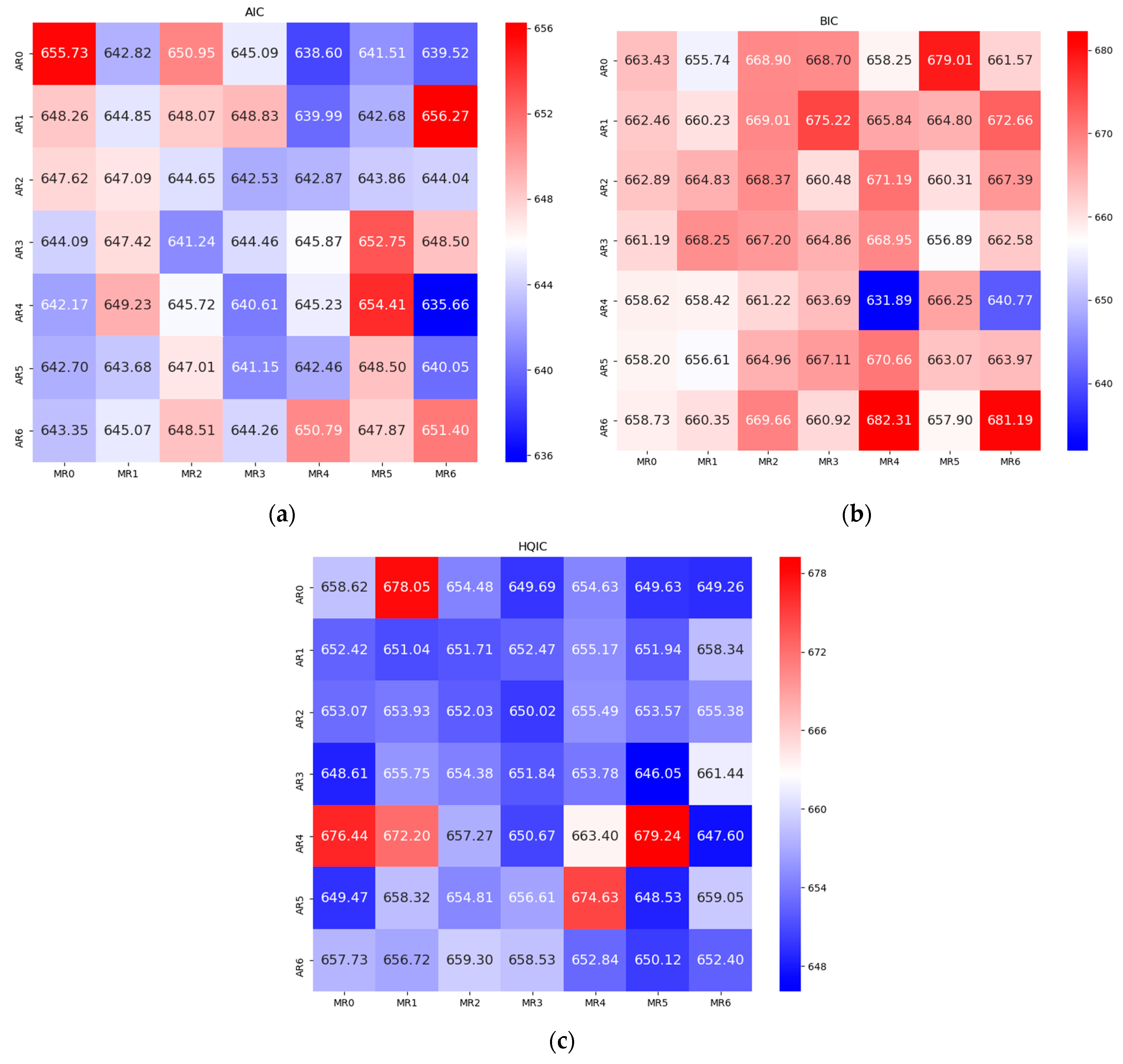
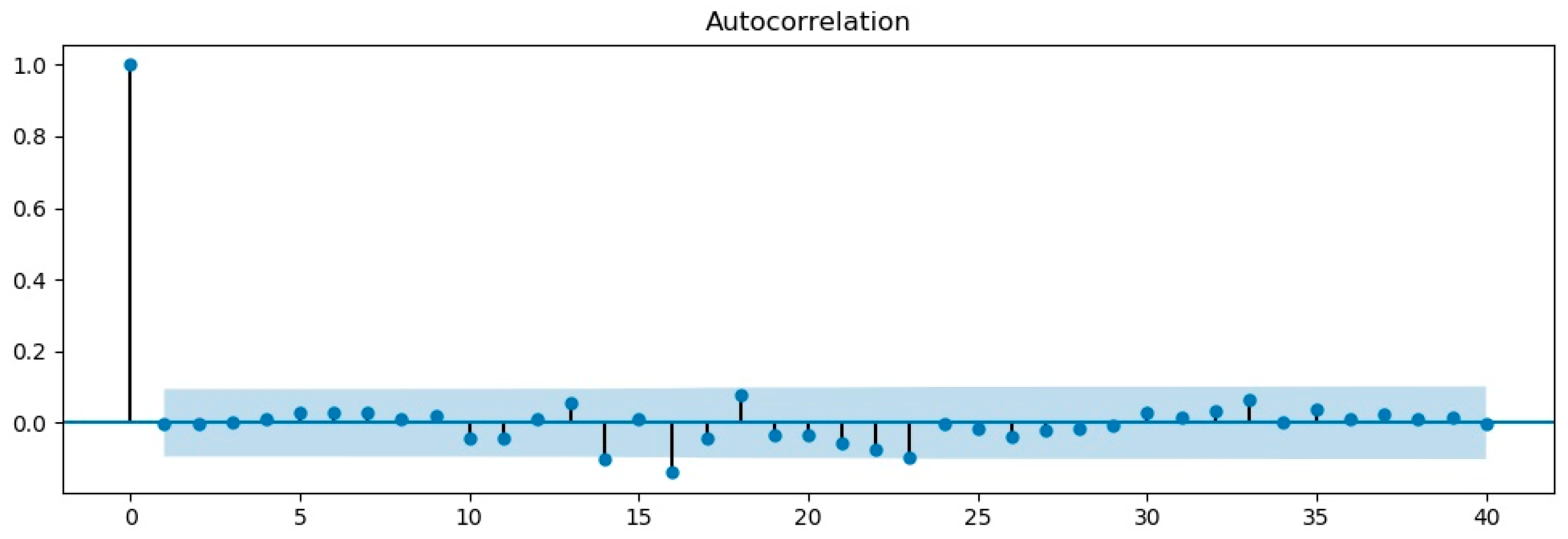
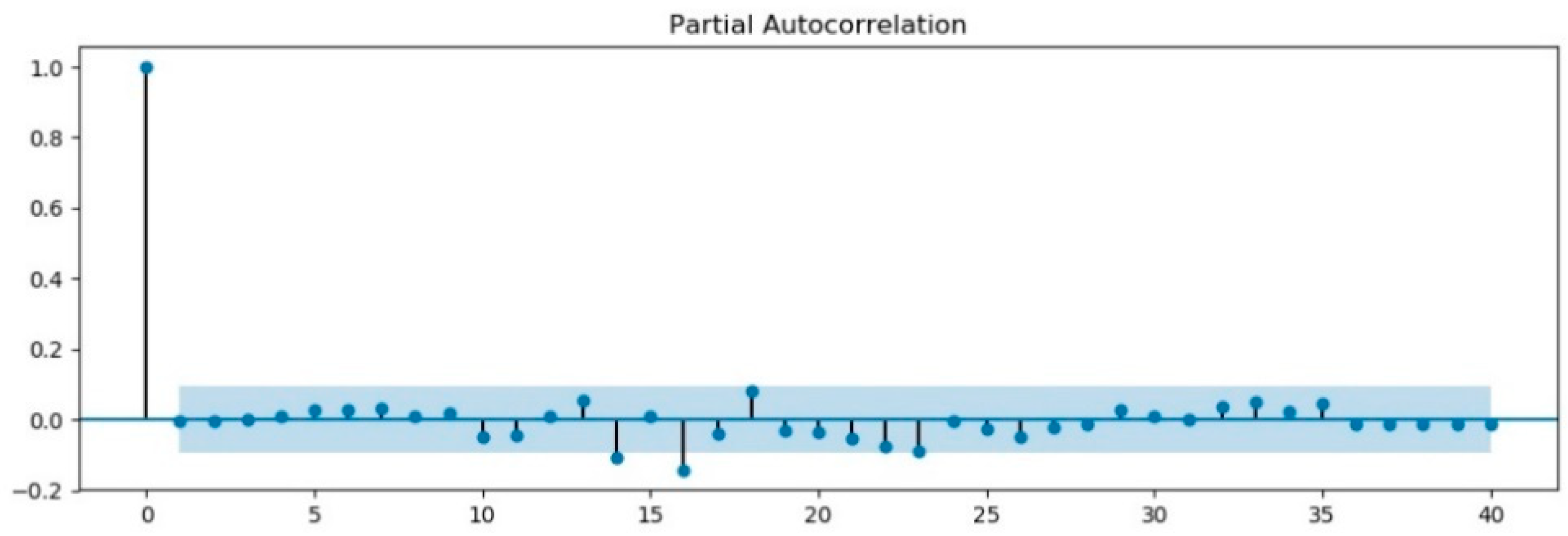
3.1. ARIMA Model
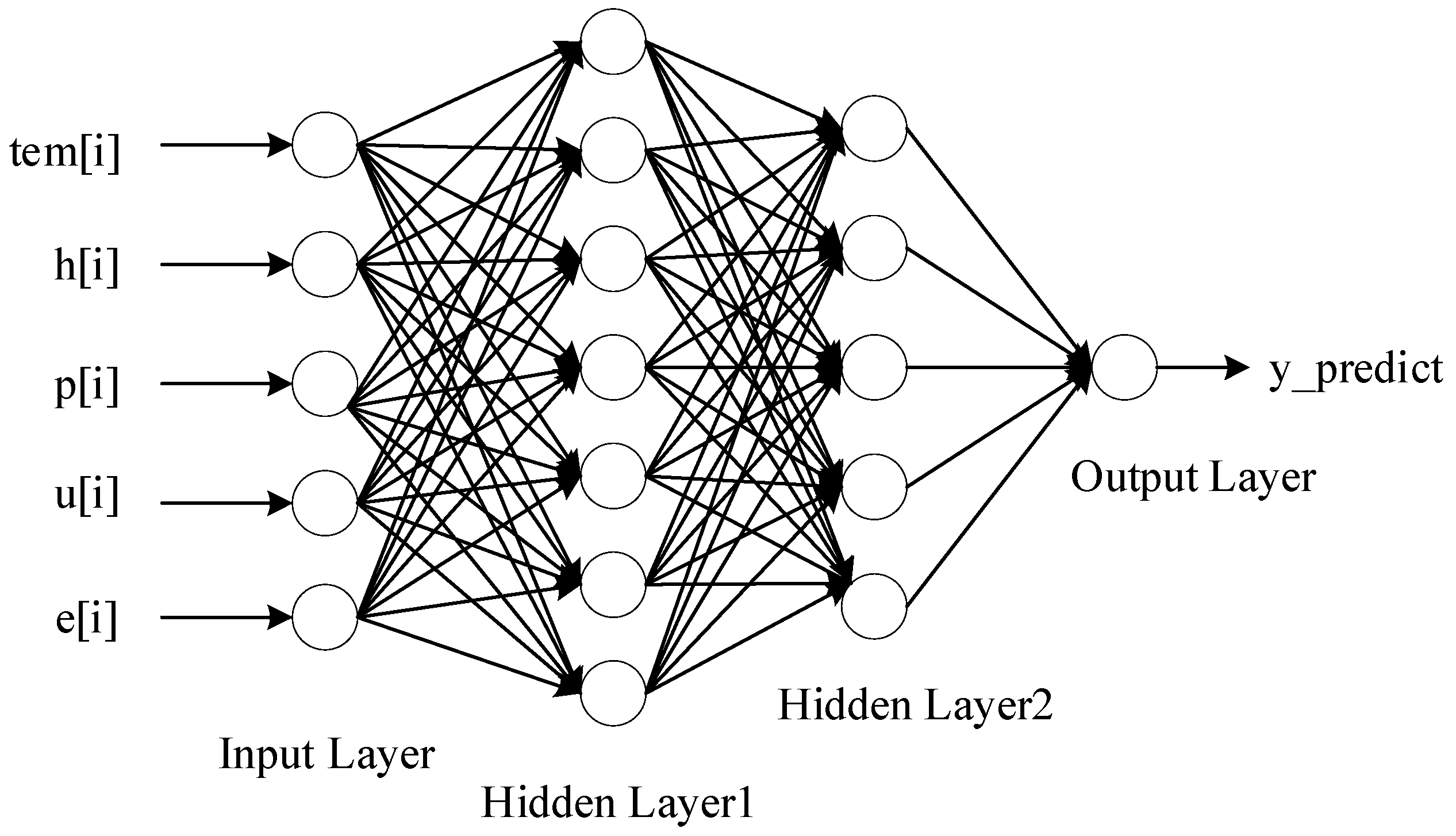
3.2. BPNN
4. CO2 Emission-Concentration Prediction with Spatiotemporal Coupled Properties Based on ARIMA-BPNN
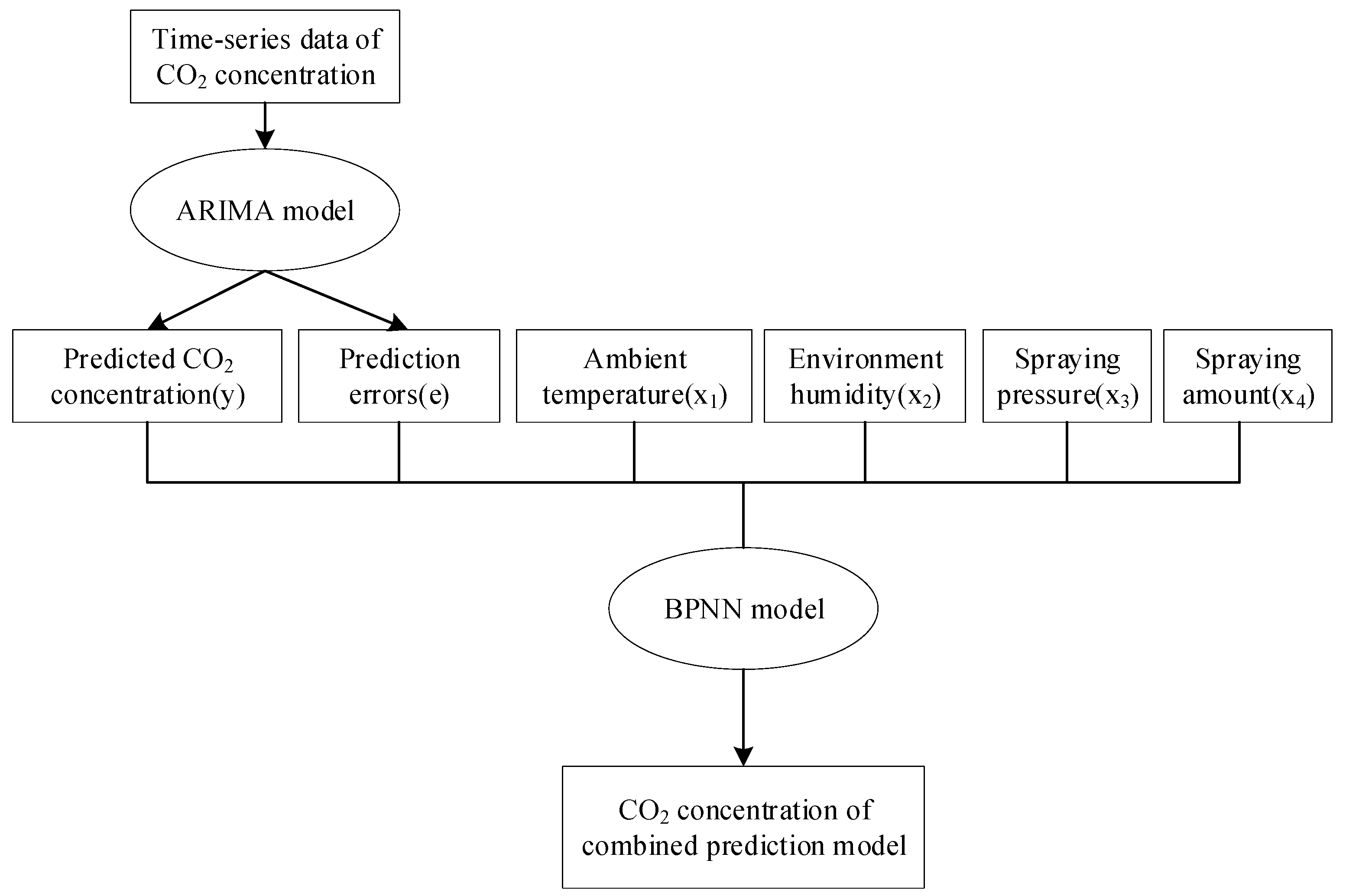
4.1. Construction of the ARIMA-BPNN Hybrid Model
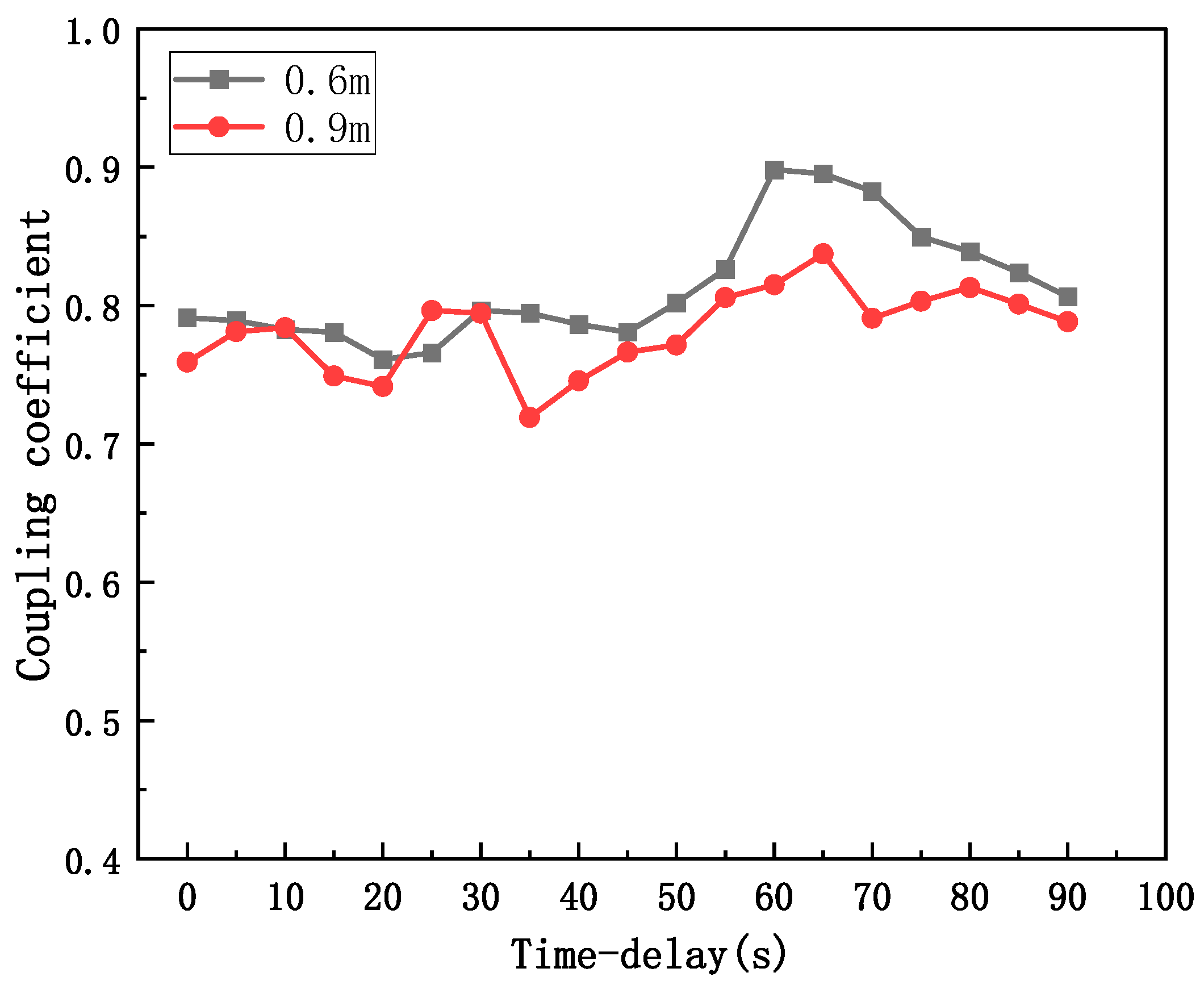
4.2. Calculation of CO2 Concentration Spatiotemporal Coupling
4.3. Prediction of the Concentration of Released CO2 Micro/Nanobubbles
| Algorithm 1 ARIMA |
| Require: x |
| Ensure: y |
| 1: for i = 0; i < 7; i++ do |
| 2: if ad f(x) = true then |
| 3: x ← Dif f |
| 4: break |
| 5: else |
| 6: x ← Dif ference(x) |
| 7: continue |
| 8: p, q ← AIC (x), BIC(X), HQIC(x) |
| 9: y ← ARIMA (x, p, d, q) |
| Algorithm 2 BPNN |
| Require: y, x, net |
| Ensure: result |
| 1: x[i] ← {tem[i], h[i], p[i], u[i], y[i], e[i]} |
| 2: net.train(net, inputn, outputn) |
| 3: inputntest ← mapminmax(inputtest) |
| 4: BPsim ← sim(net, inputntest) |
| 5: result ← mapminmax(reverse, BPsim) |
5. Instance Simulation and Analysis of Results
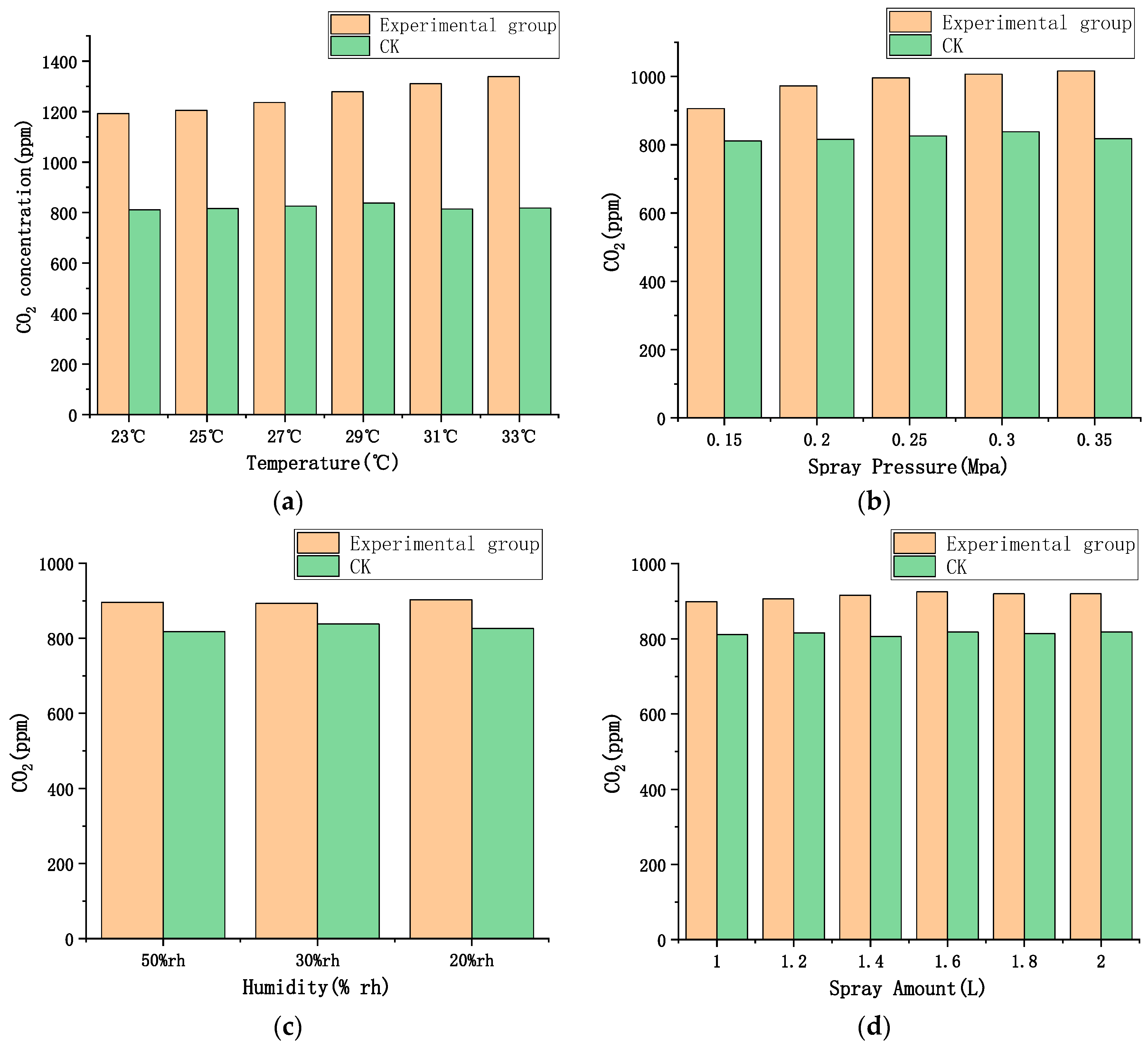
5.1. Factors Involved in CO2 Release and Dataset Selection
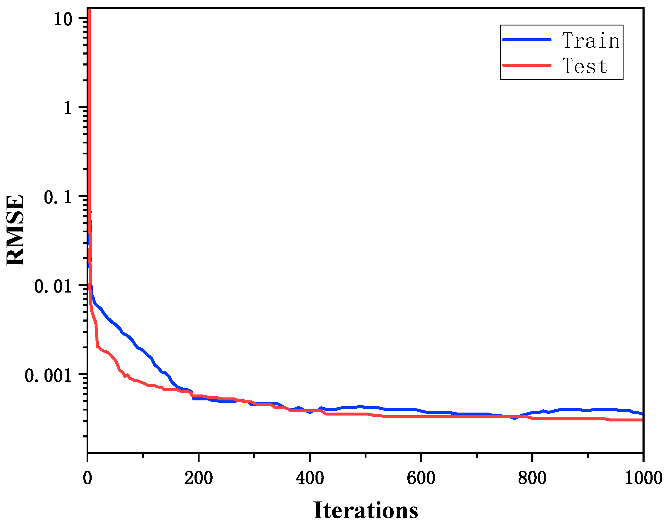
5.2. Simulation Parameters
5.3. Model Evaluation Index
5.4. CO2 Release Prediction and Analysis in Micro/Nanobubble Water
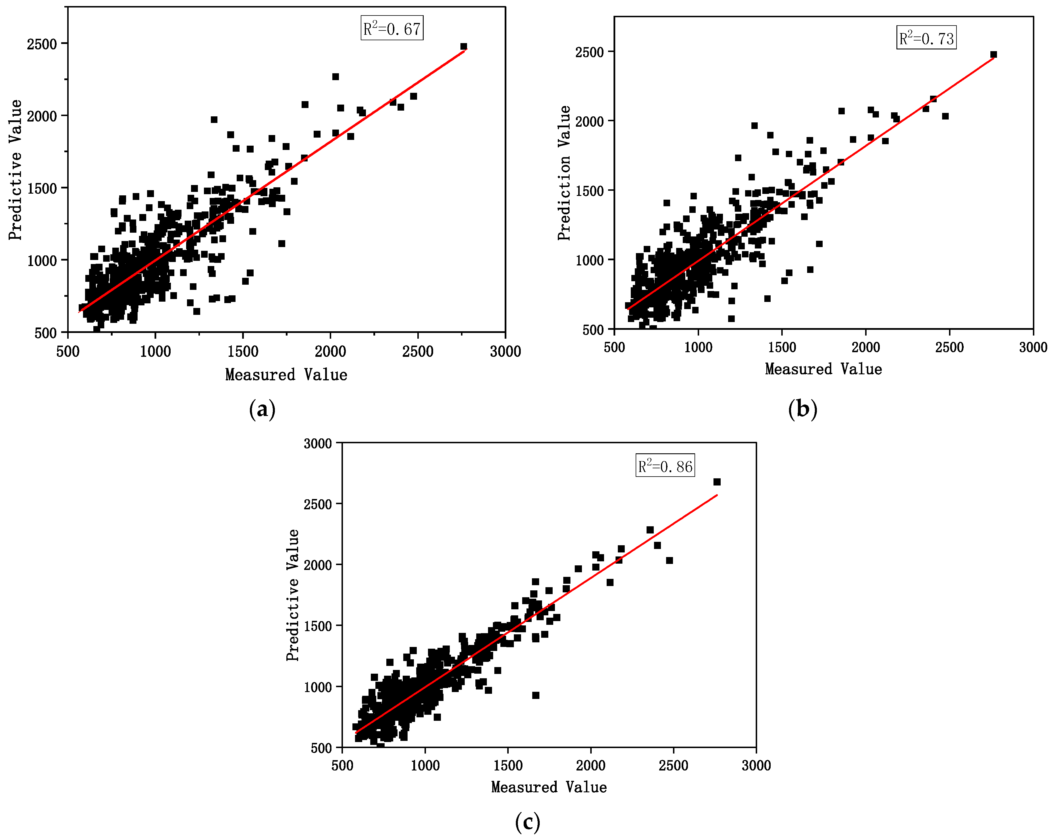
5.4.1. Model Prediction Results and Analysis
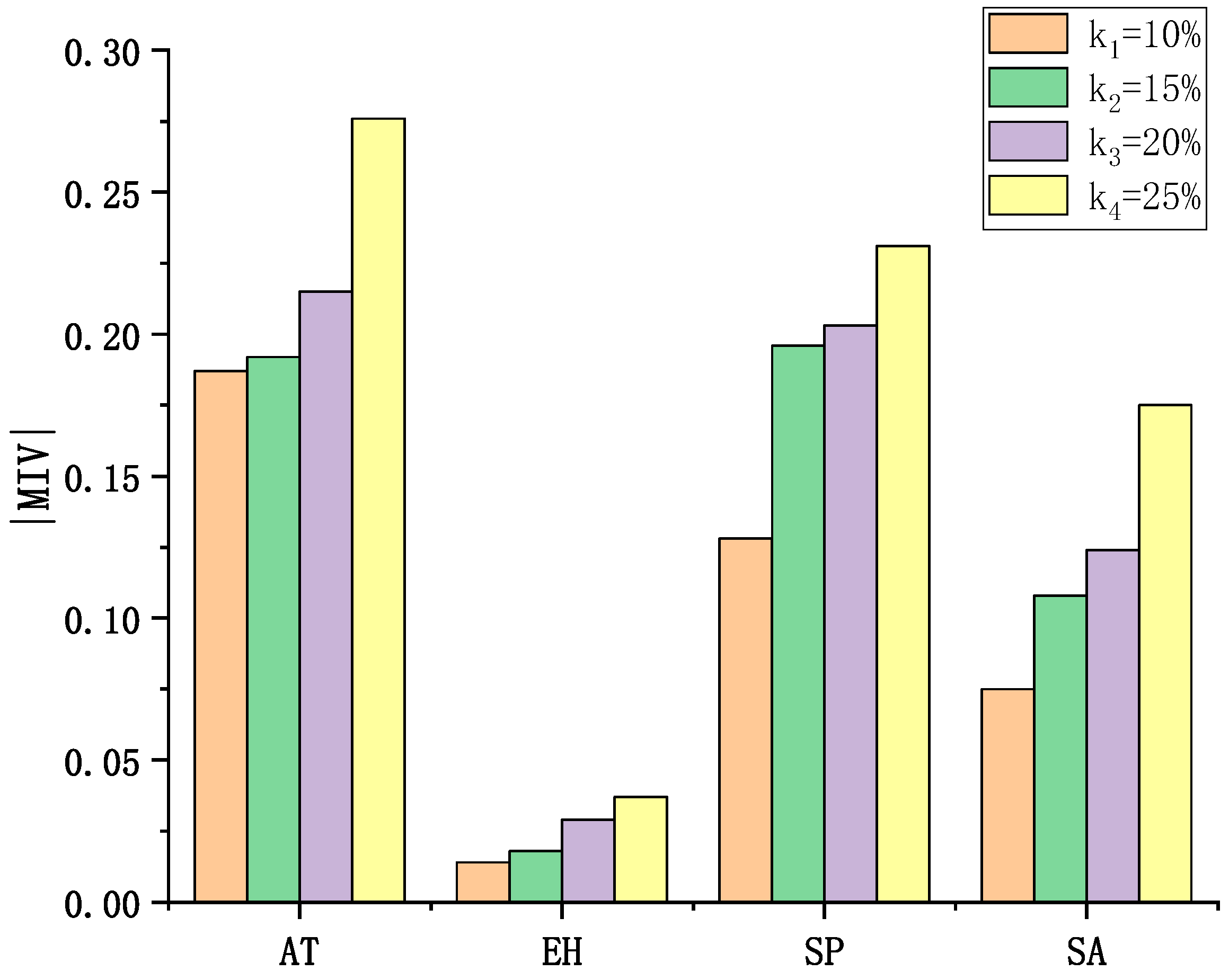
5.4.2. Analysis on Factors Affecting CO2 Release in Micro/Nanobubble Water
| Algorithm 3 MIV |
| Input: , |
| Output: , |
| 1: set adjustment rate of MIV, , , , ; |
| 2: generate a new sample dataset , ; |
| 3: use ARIMA-BPNN model to predict the new data set , , obtain the predicted results , ; |
| 4: = ; |
| 5: . |
6. Conclusions
- (1)
- Considering the linear and nonlinear properties of the gas release process, a hybrid prediction model based on the ARIMA-BPNN was constructed and compared to the prediction results of both the ARIMA and BPNN models. The results show that the fitting result based on the hybrid prediction model is the best, with R2 reaching 0.86. The RMSE and MAE values are 17.48% and 9.31%, respectively. The ARIMA-BPNN model has good prediction accuracy and could accurately fit the complex mapping relationship between the influencing elements and CO2 micro/nanobubble release concentration.
- (2)
- Based on the constructed hybrid model, the MIV algorithm was used to quantitatively analyze the influence weights of the input factors on the CO2 concentration. The experimental results show that within the range of model input variables, ambient temperature has the highest weight in the prediction model as a key factor affecting the release of CO2 micro/nanobubbles, followed by spray pressure and spray amount. The ambient humidity has the lowest weight with no significant effect.
Author Contributions
Funding
Institutional Review Board Statement
Informed Consent Statement
Data Availability Statement
Acknowledgments
Conflicts of Interest
References
- Liu, C.; Hu, Z.H.; Yu, L.F.; Chen, S.T.; Liu, X.M. Responses of photosynthetic characteristics and growth in rice and winter wheat to different elevated CO2 concentrations. Photosynthetica 2020, 58, 1130–1140. [Google Scholar] [CrossRef]
- Hussin, S.; Geissler, N.; El-Far, M.M.; Koyro, H. Effects of salinity and short-term elevated atmospheric CO2 on the chemical equilibrium between CO2 fixation and photosynthetic electron transport of Stevia rebaudiana Bertoni. Plant Physiol. Biochem. 2017, 118, 178–186. [Google Scholar] [CrossRef] [PubMed]
- Temesgen, T.; Bui, T.T.; Han, M.; Kim, T.; Park, H. Micro and nanobubble technologies as a new horizon for water-treatment techniques: A review. Adv. Colloid. Interface Sci. 2017, 246, 40–51. [Google Scholar] [CrossRef] [PubMed]
- Takahashi, M. ζ potential of microbubbles in aqueous solutions: Electrical properties of the gas-water interface. J. Phys. Chem. B 2005, 109, 21858–21864. [Google Scholar] [CrossRef] [PubMed]
- Kulkarni, A.A.; Joshi, J.B. Bubble formation and bubble rise velocity in gas-liquid systems: A review. Ind. Eng. Chem. Res. 2005, 44, 5873–5931. [Google Scholar] [CrossRef]
- Parkinson, L.; Sedev, R.; Fornasiero, D.; Ralston, J. The terminal rise velocity of 10–100 μm diameter bubbles in water. J. Colloid. Interface Sci. 2008, 322, 168–172. [Google Scholar] [CrossRef]
- Zimmerman, W.B.; Tesař, V.; Bandulasena, H.H. Towards energy efficient nanobubble generation with fluidic oscillation. Curr. Opin. Colloid. Interface Sci. 2011, 16, 350–356. [Google Scholar] [CrossRef]
- Cerrón-Calle, G.A.; Magdaleno, A.L.; Graf, J.C.; Apul, O.G.; Garcia-Segura, S. Elucidating CO2 nanobubble interfacial reactivity and impacts on water chemistry. J. Colloid. Interface Sci. 2022, 607, 720–728. [Google Scholar] [CrossRef]
- Zhang, Y.; Yasutake, D.; Hidaka, K.; Kitano, M.; Okayasu, T. CFD analysis for evaluating and optimizing spatial distribution of CO2 concentration in a strawberry greenhouse under different CO2 enrichment methods. Comput. Electron. Agric. 2020, 179, 105811. [Google Scholar] [CrossRef]
- Moon, T.; Choi, H.Y.; Jung, D.H.; Chang, S.H.; Son, J.E. Prediction of CO₂ Concentration via Long Short-Term Memory Using Environmental Factors in Greenhouses. Hortic. Sci. Technol. 2020, 38, 201–209. [Google Scholar] [CrossRef]
- Hamrani, A.; Akbarzadeh, A.; Madramootoo, C.A. Machine learning for predicting greenhouse gas emissions from agricultural soils. Sci. Total Environ. 2020, 741, 140338. [Google Scholar] [CrossRef] [PubMed]
- Benos, L.; Tagarakis, A.C.; Dolias, G.; Berruto, R.; Kateris, D.; Bochtis, D. Machine learning in agriculture: A comprehensive updated review. Sensors 2021, 21, 3758. [Google Scholar] [CrossRef] [PubMed]
- Jha, G.K.; Sinha, K. Agricultural price forecasting using neural network model: An innovative information delivery system. Agric. Econ. Res. Rev. 2013, 26, 229–239. [Google Scholar] [CrossRef] [Green Version]
- Zhou, T.; Wang, F.; Yang, Z. Comparative analysis of ANN and SVM models combined with wavelet preprocess for groundwater depth prediction. Water 2017, 9, 781. [Google Scholar] [CrossRef] [Green Version]
- Xiang, Y.; Gou, L.; He, L.; Xia, S.; Wang, W. A SVR–ANN combined model based on ensemble EMD for rainfall prediction. Appl. Soft Comput. 2018, 73, 874–883. [Google Scholar] [CrossRef]
- Zou, P.; Yang, J.; Fu, J.; Liu, G.; Li, D. Artificial neural network and time series models for predicting soil salt and water content. Agric. Water Manag. 2010, 97, 2009–2019. [Google Scholar] [CrossRef]
- Cheng, W.; Zhou, Y.; Guo, Y.; Hui, Z.; Cheng, W. Research on prediction method based on ARIMA-BP combination model. In Proceedings of the 2019 3rd International Conference on Electronic Information Technology and Computer Engineering (EITCE), Xiamen, China, 18–20 October 2019; pp. 663–666. [Google Scholar]
- Phan, K.K.T.; Truong, T.; Wang, Y.; Bhandari, B. Formation and Stability of Carbon Dioxide Nanobubbles for Potential Applications in Food Processing. Food Eng. Rev. 2021, 13, 3–14. [Google Scholar] [CrossRef]
- Tomiyama, A.; Celata, G.P.; Hosokawa, S.; Yoshida, S. Terminal velocity of single bubbles in surface tension force dominant regime. Int. J. Multiph. Flow 2002, 28, 1497–1519. [Google Scholar] [CrossRef]
- Yang, H.; Li, X.; Qiang, W.; Zhao, Y.; Zhang, W.; Tang, C. A network traffic forecasting method based on SA optimized ARIMA–BP neural network. Comput. Netw. 2021, 193, 108102. [Google Scholar] [CrossRef]
- Fan, D.; Sun, H.; Yao, J.; Zhang, K.; Yan, X.; Sun, Z. Well production forecasting based on ARIMA-LSTM model considering manual operations. Energy 2021, 220, 119708. [Google Scholar] [CrossRef]
- Wang, F.; Zou, Y.; Zhang, H.; Shi, H. House price prediction approach based on deep learning and ARIMA model. In Proceedings of the 2019 IEEE 7th International Conference on Computer Science and Network Technology (ICCSNT), Dalian, China, 19–20 October 2019; pp. 303–307. [Google Scholar]
- Zhai, M.; Li, W.; Tie, P.; Wang, X.; Xie, T.; Ren, H.; Zhang, Z.; Song, W.; Quan, D.; Li, M.; et al. Research on the predictive effect of a combined model of ARIMA and neural networks on human brucellosis in Shanxi Province, China: A time series predictive analysis. BMC Infect. Dis. 2021, 21, 280. [Google Scholar] [CrossRef] [PubMed]
- Wang, Z.; Ding, Y. Research on Signal-to-Noise Ratio in Order Selection of AR Model. Acta Math. Sci. (Ser. A) 2020, 40, 811–823. [Google Scholar]
- Bierens, H.J. Information Criteria and Model Selection; Pennsylvania State University: State College, PA, USA, 2004. [Google Scholar]
- Wang, Z.; Liu, S.; Feng, L.; Xu, Y. BNNmix: A new approach for predicting the mixture toxicity of multiple components based on the back-propagation neural network. Sci. Total Environ. 2020, 738, 140317. [Google Scholar] [CrossRef] [PubMed]
- Jiang, B.; Liu, H.; Xing, Q.; Cai, J.; Zheng, X.; Li, L.; Liu, S.; Zheng, Z.; Xu, H.; Meng, L. Evaluating traditional empirical models and BPNN models in monitoring the concentrations of chlorophyll-A and total suspended particulate of eutrophic and turbid waters. Water 2021, 13, 650. [Google Scholar] [CrossRef]
- Zhao, J.; Yang, D.; Wu, J.; Meng, X.; Li, X.; Wu, G.; Miao, Z.; Chu, R.; Yu, S. Prediction of temperature and CO concentration fields based on BPNN in low-temperature coal oxidation. Thermochim. Acta 2021, 695, 178820. [Google Scholar] [CrossRef]
- Kumari, N.; Belwal, R. Hybridized approach of image segmentation in classification of fruit mango using BPNN and discriminant analyzer. Multimed. Tools Appl. 2021, 80, 4943–4973. [Google Scholar] [CrossRef]
- Wang, J.; Fang, J.; Zhao, Y. Visual prediction of gas diffusion concentration based on regression analysis and BP neural network. J. Eng. 2019, 2019, 19–23. [Google Scholar] [CrossRef]
- Liu, M.; Ding, L.; Bai, Y. Application of hybrid model based on empirical mode decomposition, novel recurrent neural networks and the ARIMA to wind speed prediction. Energy Convers. Manag. 2021, 233, 113917. [Google Scholar] [CrossRef]
- Qi, Y.; Li, Q.; Karimian, H.; Liu, D. A hybrid model for spatiotemporal forecasting of PM2. 5 based on graph convolutional neural network and long short-term memory. Sci. Total Environ. 2019, 664, 1–10. [Google Scholar] [CrossRef]
- Wang, W.; Du, Y.; Chau, K.; Chen, H.; Liu, C.; Ma, Q. A Comparison of BPNN, GMDH, and ARIMA for Monthly Rainfall Forecasting Based on Wavelet Packet Decomposition. Water 2021, 13, 2871. [Google Scholar] [CrossRef]
- Berkhin, P. A Survey of Clustering Data Mining Techniques; Springer: Berlin/Heidelberg, Germany, 2006; pp. 25–71. [Google Scholar]
- Wu, T.; Zhan, J.; Yan, W. Research on influence factors of real estate price based on MIV-BP neural network test. Math. Pract. Theory 2015, 18, 45–52. [Google Scholar]


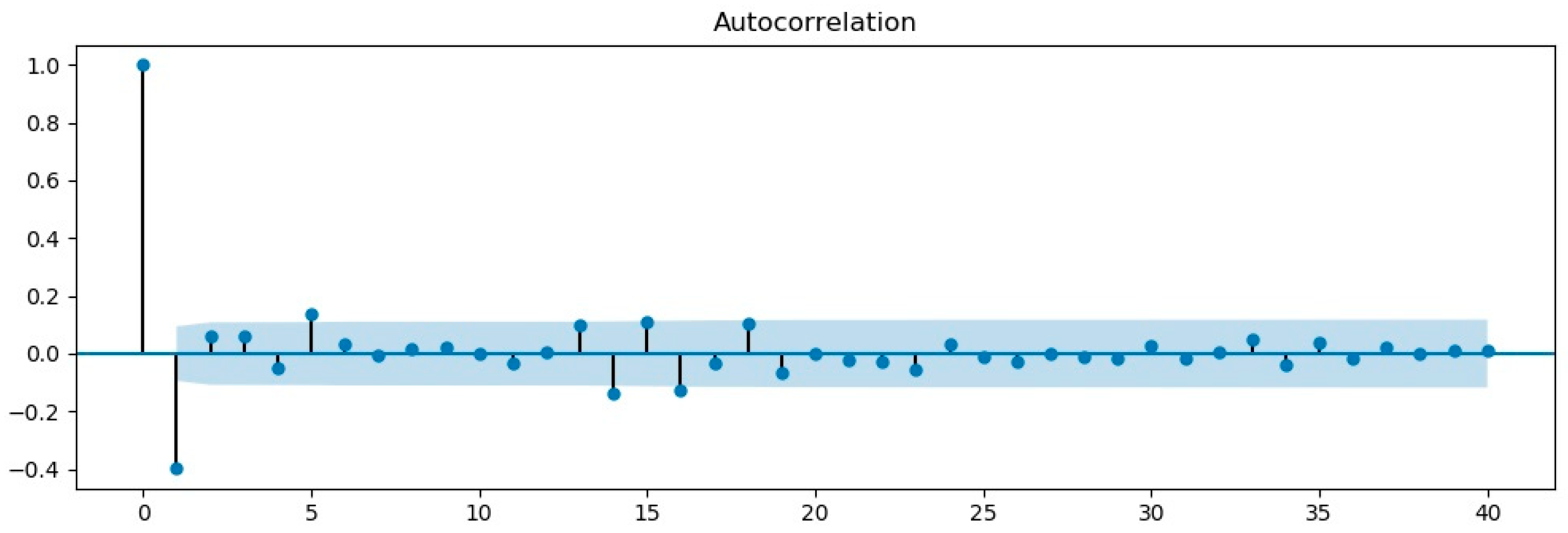
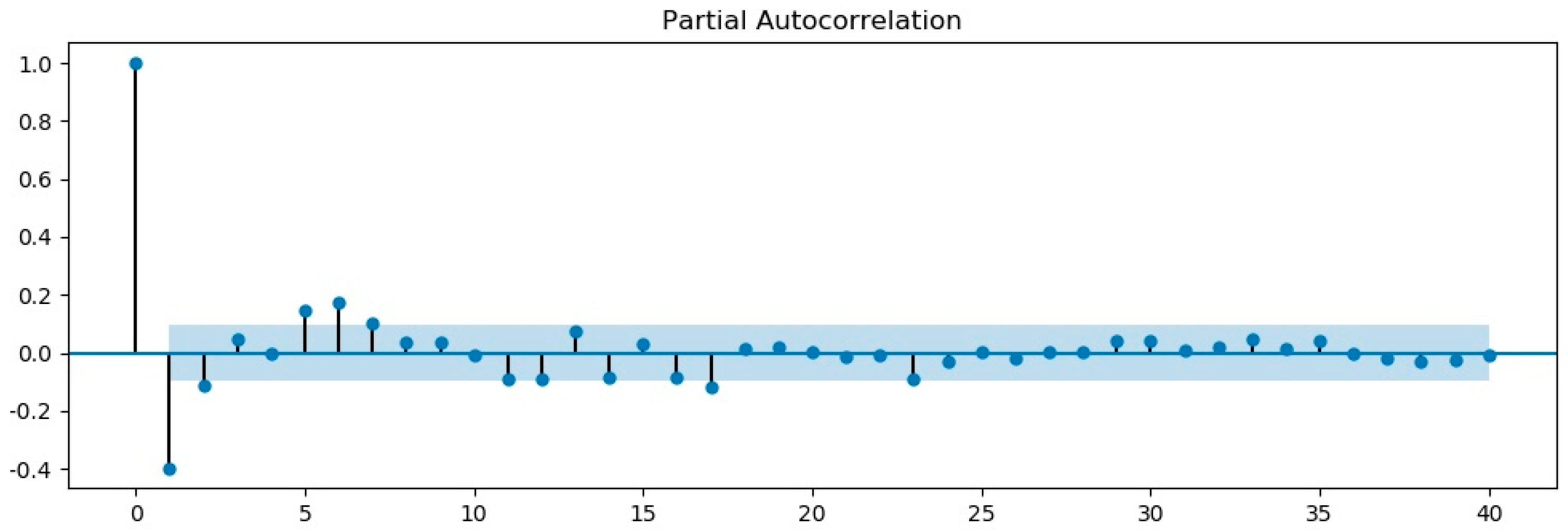
| Comparison Item | ADF | 1% Significance Level | 5% Significance Level | 10% Significance Level |
|---|---|---|---|---|
| Before first-order difference test | −0.6987 | −3.16 | −2.89 | −2.85 |
| First-order difference test | −24.44 | −3.44 | −2.87 | −2.57 |
| Parameter | Value |
|---|---|
| Activation function | tan-sigmoid |
| Training function | traingdx |
| Loss function | L2 loss |
| Optimizer | SGD (stochastic gradient descent) |
| Learning rate | 0.01 |
| Iterations | 1000 |
| Model | RMSE | MAE |
|---|---|---|
| BPNN | 38.77 | 29.51 |
| ARIMA | 42.82 | 33.58 |
| ARIMA-BPNN | 17.48 | 9.31 |
Publisher’s Note: MDPI stays neutral with regard to jurisdictional claims in published maps and institutional affiliations. |
© 2022 by the authors. Licensee MDPI, Basel, Switzerland. This article is an open access article distributed under the terms and conditions of the Creative Commons Attribution (CC BY) license (https://creativecommons.org/licenses/by/4.0/).
Share and Cite
Wang, B.; Lu, X.; Ren, Y.; Tao, S.; Gao, W. Prediction Model and Influencing Factors of CO2 Micro/Nanobubble Release Based on ARIMA-BPNN. Agriculture 2022, 12, 445. https://doi.org/10.3390/agriculture12040445
Wang B, Lu X, Ren Y, Tao S, Gao W. Prediction Model and Influencing Factors of CO2 Micro/Nanobubble Release Based on ARIMA-BPNN. Agriculture. 2022; 12(4):445. https://doi.org/10.3390/agriculture12040445
Chicago/Turabian StyleWang, Bingbing, Xiangjie Lu, Yanzhao Ren, Sha Tao, and Wanlin Gao. 2022. "Prediction Model and Influencing Factors of CO2 Micro/Nanobubble Release Based on ARIMA-BPNN" Agriculture 12, no. 4: 445. https://doi.org/10.3390/agriculture12040445
APA StyleWang, B., Lu, X., Ren, Y., Tao, S., & Gao, W. (2022). Prediction Model and Influencing Factors of CO2 Micro/Nanobubble Release Based on ARIMA-BPNN. Agriculture, 12(4), 445. https://doi.org/10.3390/agriculture12040445