Abstract
Assessing the risk of using pesticides for the environment in general, and for groundwater in particular, necessitates prediction of pesticide migration. For this purpose, mathematical models of pesticide behavior are utilized, which must be parameterized and calibrated based on experimental data to make them perform properly. The behavior of the pesticide cyantraniliprole was examined in a long-term lysimetric experiment. The MACRO 5.2 dual porosity model was calibrated based on the percolate and the levels of pesticides in the soil profile and percolate. Despite employing experimentally verified soil parameters and pedotransfer functions (PTF), the model must be calibrated for percolation. This is due to the model’s properties as well as the complexity of the soil as an object of study, and its pore space, which is subject to daily and annual fluctuations. It is the parameters that describe the structure of the pore space that need to be calibrated. Calibrating for pesticide concentrations required a minor revision of the sorption and transformation rates, as well as an increase in the dispersivity and ASCALE values.
Keywords:
soil; pesticide fate model; pesticide; movement; leachate; preferential flow; lysimetric studies 1. Introduction
Conservation of the environment is a major challenge of our time. The use of crop protection products in agriculture often entails contamination of groundwater, as evidenced by monitoring data [1,2,3,4]. Pesticide leaching can be as high as 5% but is typically less than 1% of the amount applied [5]. Predicting the migration of pesticides makes it possible to prevent undesirable effects of their application and take measures to reduce the adverse effects.
Since the 1980s, over a hundred models have been designed to predict the behavior of pesticides in the environment. These models are widely used not only for research purposes but also to support the pesticide registration process. Four of them were recommended by the FOCUS group (FOrum for Co-ordination of pesticide fate models and their USe) for risk assessment of pesticides during their registration in the EU [6]: MACRO [7], PEARL [8], PELMO [9] and PRZM [10]. In Russia, the PEARL leaching model is used in the risk assessment procedure. This model belongs to the chromatographic type and uses the Richards equation and the convection-dispersion-diffusion equation to describe the transport of water and solutes in soil, respectively. However, the ability of chromatographic models to predict pesticide movement in cracking clay soil has proven to be low [11,12,13]. In well-structured soils, due to the presence of macropores, dissolved substances move with the preferential flow which entails the discrepancy between the measured and predicted distribution profiles of substances, as well as the occurrence and the increased presence of the pesticides in the percolate [12]. In the version of the PEARL 4.4.4 model, a macropore transport component was added to the convection-diffusion transport. However, users do not have the opportunity to independently parameterize the equations describing the segregation of pores into macro- and microdomains [14].
Similar studies were carried out not only for soils but also for layered sediments [15,16]. The results of Vassena et al. [16] showed the presence of typical preferential flow in alluvial deposits in the presence of associated permeable structures and the applicability of the two-domain approach to their calculation with the division of the porous medium into fast and slow regions, characterized by high and low hydraulic conductivity, respectively.
Therefore, it is of both a research and practical interest to study the movement of pesticides in the soil using dual-permeability models, which are represented by the MACRO 5.2 [7]. MACRO 5.2 divides total soil porosity into two domains (micropores and macropores), each characterized by its own volume of percolate and solute concentrations. The borderline between the domains is defined by the boundary moisture content, surface tension, and hydraulic conductivity.
Water transport in micropores (intra-aggregate pores) is described by the Richards equation, and in macropores by the kinematic wave approach. The convection-dispersion-diffusion equation is used to model solute transport in micropores; in macropores, water flow is considered to be exclusively convective [7].
Apart from MACRO, there are other pesticide migration models currently available that take into account the movement of solutes with preferential flow (e.g., RZWQM and HYDRUS-1D). However, it should be noted that MACRO is the most efficient in terms of input parameter requirements, as it requires only four additional parameters to describe water flow in macropores compared to models based on the Richards equation and the convection-diffusion equation [17]. Thus, the model requires the values of soil characteristics such as micropore saturated water content (θb), boundary hydraulic conductivity (KSM), effective diffusion path length (ASCALE), and macropore size distribution factor (ZN).
Calibration of pesticide leaching models in soil, as a rule, consists of two stages: firstly, the water flow model and then the pesticide fate model are calibrated [12]. At the first stage, the model is calibrated by matching the observed and predicted values of water content and percolation. First and foremost, the calibration concerns those parameters that are difficult or impossible to measure directly in the experiment, such as qconst, which determine flow into groundwater, d-aggregate radius, and n*-value of the exponent in the kinematic wave equation or when measured, there is a high uncertainty-KSM (hydraulic conductivity in micropores) and KSATMIN (hydraulic conductivity).
Differences between the observed and predicted percolation (or water content) are evaluated by the ME model efficiency value or other fit/mismatch parameters (e.g., coefficient of variation (NRMSE—scaled root mean square error), sum of squared deviations, CRM (coefficient of residual mass), etc. The values of each parameter change within theoretically acceptable limits until an optimal match can be achieved.
The input values of the half-life (DT50) and sorption constant (Koc) of the pesticide are calibrated at the second stage. The parameters of sorption and degradation are subject to calibration because they significantly affect the final result, i.e., the residues of the pesticide in the soil, its distribution in the soil profile and its concentration in percolate [18]. In addition, sorption and degradation parameters in the laboratory are usually determined in disturbed soils, so it is not possible to directly extrapolate their results to structured soils in the field [19,20]. Additionally, it should be kept in mind during the calibration that if two parameters are correlated, only one of them can be calibrated.
The literature review shows that the most sensitive parameters requiring calibration are ASCALE (effective diffusion index), KSATMIN and KMS (filtration coefficient and microporous filtration coefficient), kinematic index and the parameter that determines seepage to groundwater [21], XMPOR (micropore water saturation) and STEN (soil moisture stress at the boundary between macro- and micropores) [22], Van-Genuchten equation parameters [23,24] and coefficients describing dispersion [25].
Calibration is carried out both using automated [21,22] and manual procedures [24,25,26]. The work of Baratelli et al. [27] proposed an improved model calibration procedure that allows the interpretation of data from numerical transport experiments using a two-domain approach, which can be useful for modeling the effects of preferred flow paths. The fitting accuracy is usually determined using statistical criteria [25,26,27,28], as well as a graphical representation of the result to assess the discrepancy between calculated and measured values [29].
Based on the results of the mentioned studies, we can conclude that describing the profile distribution of moisture, bromide, and pesticides is a more achievable task than predicting percolation and the concentrations of substances in it [30]. Based on all of the above, we can conclude that pesticide fate models need calibrating. Calibration makes it possible to improve the prediction accuracy for the available data set, as well as to determine the values of a number of parameters that are difficult to determine experimentally (inverse modelling). By and large, model calibration is an art, and as such it requires some feeling and experience on the part of the researcher, although its basic principles are known. As can be seen from the above-mentioned works, researchers have calibrated models with different parameters, across different data sets, and using different goodness-of-fit criteria. There seems to be insufficient data to date to bring the MACRO model calibration approaches to some uniformity. In addition, it remains unclear whether the model, once calibrated, will adequately predict targets (percolation and IPU concentration), since in a study by Nolan et al. [22] the calibrated model for one data set gave a better prediction than for another.
The purpose of this study was to investigate the features of modeling the transport of matter in soils, taking into account changes in conditions at the upper boundary, the transformation of the pore space and evolutionary processes and to evaluate the ability of MACRO (v.5.2) in simulating water and pesticide movement as measured in a lysimetric experiment.
2. Materials and Methods
2.1. Pesticide
Cyantraniliprole is a second generation anthranilic diamide insecticide. It is effective against various sucking pests and thrips, as well as against lepidopterous pests at the same level as first-generation anthranylamide insecticides (chlorantraniliprole).
Cyantraniliprole has a wide spectrum of activity: it acts against important agricultural pests such as caterpillars, whiteflies, miners, flies, beetles, and aphids. Various formulations containing cyantraniliprole are suitable for both vegetation and soil application. Formulations with cyantraniliprole are used for growing eggplants, tomatoes, peppers, cucumbers, peas, salad, potatoes, leeks, onions, fruit, peaches, apricots, grapes and cherries. In the Russian Federation, 4 monoformulations containing cyantraniliprole are registered: Benevia, OD (100 g/L) and Verimarc, SC (200 g/L) for application during vegetation, and Lumiposa, TC (625 g/L) and Fortenza, SC (600 g/L) for seed treatment, and in a mixture with abamectin Lyrum, SC (60 18 g/L).
Cyantraniliprole is a weak acid (pKa = 8.80 1.38 at 20 °C), has low water solubility (14.2 mg/L), low volatility (vapor pressure 5.13 × 10⁻¹² mPa) [31]. It has low mammalian toxicity and low bioaccumulation potential (Log P = 2.02 at pH = 7 at 20 °C). It is highly toxic to honey bees, moderately toxic to earthworms and most aquatic species, rapidly degraded in water by photolysis (DT50 = 0.22 d), but moderately resistant to hydrolysis (DT50 = 61 d), persistence in soil varies from low to high (DT50 8.7–91.9 in laboratory conditions) and sorption coefficient is moderate 157–361 [31].
To parameterize the model, half-life values DT50 = 49.9 d [32] and distribution coefficient normalized by organic carbon content, Kos = 387 mL/g [33], were used from laboratory experiment in Albic Glossic Retisols soil (Moscow region).
2.2. Lysimeter Experiment
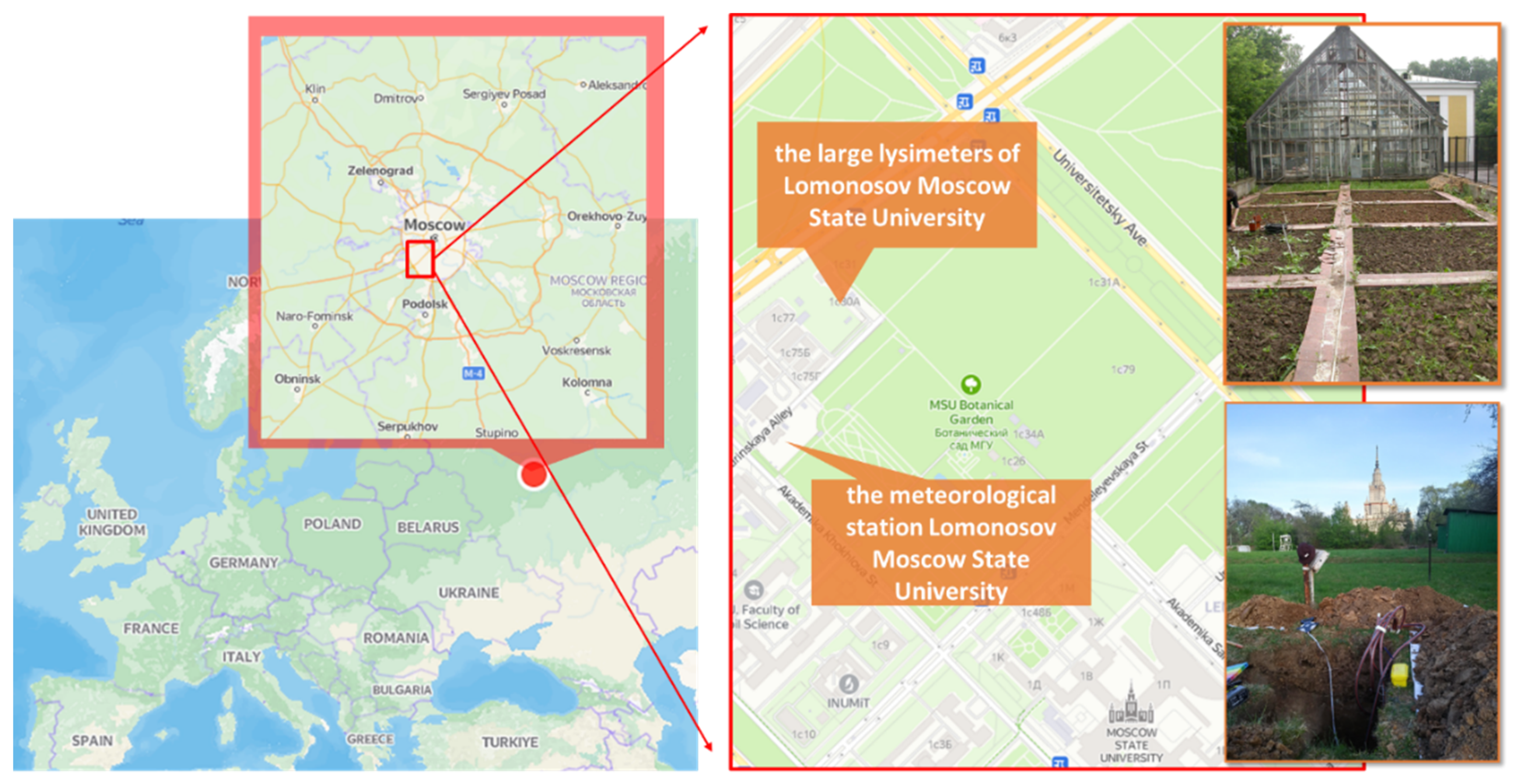
The experiment was carried out in the large lysimeters of Lomonosov Moscow State University (Moscow, Russia, 55°42′31.9″ N 37°31′25.1″ E, Figure 1. Cyantraniliprole was used with a backpack sprayer in the recommended (0.4 kg ha−1) and ten-fold (4.0 kg/ha) application rates twice in June 2015 and June 2016. More details of the experiment are described in our previous work [32].

Figure 1.
Location and appearance of lysimeters.
2.3. Pesticide Analysis
The method of cyantraniliprole analysis is based on the extraction thereof from water with n-hexane, purification of the extracts obtained with C8 cartridges and the subsequent determination of cyantraniliprole by high-efficiency liquid chromatography (HPLC) using a UV detector at 265 nm. Limit of determination of cyantraniliprole was 0.5 mgk/l.
2.4. Model MACRO (Version 5.2)
The MACRO model is a dual-permeability model that divides the porous space into two domains—macropores and micropores—each characterized by its own flow rate and concentration of substances [34,35]. In micropores (i.e., intra-aggregate pores), the movement of water is described by the Richards equation, and the transport of solution by the convective-diffusion equation. For transport over macropores, the kinematic wave equation is used, which means that movement does not observe the phenomena of dispersion and diffusion, but is considered exclusively convective [7,34]. Macropores permeate the soil profile throughout the depth, in the micropore domain it takes into account the process of non-equilibrium sorption and uses the two-site model [34,35]. The boundary between the macropores and the micropores domain is defined in the model by the boundary moisture content, surface tension and hydraulic conductivity. Water enters the macropores as soon as the infiltration capacity of the micropores (topsoil) or the boundary water content (remaining profile) is exceeded [36].
2.5. Model Parameters of MACRO
The soil profile was divided into 6 horizons and the main soil properties are depicted in Table 1. The input parameters of the water model of the MACRO are presented in Table 2.

Table 1.
Some chemical and physical properties of the Albic Glossic Retisol of lysimeter.
Table 2.
Hydraulic parameters of Albic Glossic Retisol for MACRO 5.2.
The parameters of the water retention curve (WRC) approximation by the van Genuchten equation were calculated using the RETC model. The water retention curve was determined in the laboratory for the top two layers, data for horizons below 20 cm were taken from the literature [24,37]. The ASCALE parameter was also set according to gradations based on soil structure [38]. The CTEN value is set on the basis of the clay content of the profile, for soil clay content between 10 and 15% CTEN is equal 12 cm, with a lower CTEN content is 10 cm [38]. The saturated hydraulic conductivity for lysimeter soil is taken from literary sources [37]. The saturated hydraulic conductivity in micropores can be estimated from soil texture, which is automatically determined in the model with the input of the particle-size distribution.
However, the guidance [38] does not contain values for silt or silt loam. Based on the correspondence of names of soil texture classes in the USDA classification to names in Russian classification [39] and according to the soil profile description [40] it was decided to use KSM 0.15 mm/h for the first 40 cm and 0.05 mm/h for the lower horizons [38].
According to the data of a tomographic study of the Albic Glossic Retisol soil of the Moscow region [41] in the humus horizon the average volume of macropores is 7.3%, and in the lower layers of macropores is 3.3%, consequently, the moisture content of the micropores was defined as the difference between the moisture content of the full saturation and the volume of macropores. The parameter ZN is 2 for clay and some coarse sands, and 4 is clay loam [38], so the upper 40 cm of ZN is 3 and the lower of the profile is 2. ZM is set to 0.5 based on the Mualem approach [7]. ZP is 0, indicating no shrinkage. ZA is set by default to 1 without shrinkage influence [7,38].
2.6. Estimation of Model Accuracy
In order to assess the accuracy of the simulation, a visual comparison of the plots of measured and predicted cumulative percolation from the lower boundary of the soil profile of lysimeters was performed, as well as the calculation of three statistical parameters: the model efficiency (EF), the residual mean squared error (RMSE) and the coefficient of residual mass (CRM):
where Pi and Oi are the predicted and observed values, respectively, is the mean of the observed (measured) values, and n is the number of measured values. The optimal values of EF, RMSE and CRM are 1, 0 and 0, respectively. Positive CRM values indicate that the model underestimates the measurement.
3. Results
3.1. Water Transport Modelling
The work on calibrating the water model of the MACRO was carried out in several stages. The first step involved the selection of the optimal calibrating range. A measurement of 565.4 mm of percolate was detected from the lower boundary of lysimeter in period from 10 June 2016 to 7 June 2017. The cumulative water flow curve is characterized by the step structure effect of rain precipitation (Figure 2, green curve). In addition, the plateau is clearly visible from November until mid-February, when the water flow was virtually non-existent, followed by a sharp rise in water flow associated with the spring snowmelt.
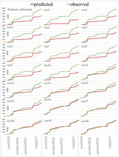
Figure 2.
Comparison of experimental (observe) and predicted percolation without/with model calibration (20 options according to Table 3).
The initial calculation in MACRO 5.2 model is performed with the input parameters described in the relevant part of the work, but in order to estimate the model prediction without any configuration, the macropores content has been calculated with the PTF built into the model. The model underestimates the total amount of percolate (Figure 2. without calibration). According to Ritter and Muñoz-Carpen [42], the model forecast is considered unsatisfactory if EF < 0.65, acceptable if 0.65 < EF < 0.80, good if 0.80 < EF < 0.90, or very good if EF ≥ 0.90. In this case, model accuracy was 0.407, so 20 options were further tested to improve the accuracy of lysimeter percolate prediction (Table 3). For each option, observe and predictive comparison graphs were drawn up (Figure 2) and statistical parameters were calculated (Table 4).
Table 3.
Hydraulic parameters used as MACRO 5.2 input and parameters to be calibrated (marked by plus).
Table 4.
Statistic parameters of simulated percolation for uncalibrated and calibrated runs.
In the next alternative forecast, the WRC parameters, the saturated hydraulic conductivity (total and in micropores) for all soil horizons were calculated by PTF embedded in the model, resulting in reduced water flow and even greater simulation errors (Figure 2 (var1)). Therefore, it was decided to return the values of all input parameters to the original, including the volume of the macropores according to the tomographic data described in Section 2.5 “Model Parameters of MACRO”. The amount of total water flow, model accuracy and model errors are very close to the data from the non-calibration model, but the experimental macroporosity data are not very different from the PTF data; for example, for the top 10 cm, according to the tomography data, the amount of macropores is approximately 7.3% in Albic Glossic Retisol, while due to PTF it is 5.96%.
Since the model is sensitive to the CTEN (soil moisture tension at the interface between the macro- and micropores) parameter, it was decided to increase the value in all horizons by 50%, resulting in a decrease in water flow (Figure 2 (var3)), and therefore its value was fixed to 10 for the entire soil profile in all subsequent calculations, since Beulke and colleagues [38] note that this parameter can be accepted in area 10 for most soils. This was followed by a two-fold increase in the number of macropores, which increased the accuracy of the model to 0.540, so the macroporosity values were doubled for later calculations. It was further checked whether the shift of the starting date of the model calculation affects the water flow, the shift of the start to June 2014 did not lead to any changes, but if the calculation start is set to June 2016, the water flow decreases, thereby confirming the fact noted in the Dubus et al. article [43] that stated the models need a “warming up period” several months before the beginning of the simulated period. The pore size distribution index was further calibrated according to the MACRO model parameter estimation guidance, the indicator in the model ranged from 2 to 6, with 2 recommended values: two for clays with a distinctly bimodal pore system, and a 4 for sandy and light loams. At Zn = 2 there was a slight increase in water flow, and Zn = 4 reduces water flow, so the parameter is also further fixed at 2.
The next parameter that can influence the flow is the saturated hydraulic conductivity in micropores—increasing this parameter to 0.52 mm/h for the upper horizon according to the PTF built into the model has led to a significant deterioration in the prediction; the precision of the model (EF) was reduced to 0.174 (Table 4), so this parameter was set to 0.05 mm/h for the whole profile, and such values are characteristic for clay. This led to an adequate prediction, and model errors decreased significantly (Table 4). The reduction of the saturated hydraulic conductivity in micropores to 0.03 mm/h increased the simulation efficiency to 0.911. The graph (Figure 2 (var12)) shows that the predicted water flow is almost the same as the experimental water flow from June to September. The calibration of this parameter thus simulates a process where most soil moisture migrates through macropore pores and cracks.
For well-structured soils, the value of the ASCALE parameter (the length of the effective diffusion path) is 30 mm, so it was decided to set this value for the topography of the soil, which allowed a slight improvement in the prediction. Increasing the saturated hydraulic conductivity by 50% to simulate a great volume of large macropores under field conditions does not affect the total amount of water flow and the curve curvature. Therefore, we leave the KSATMIN values unchanged.
Statistical prediction parameters suggest that the already available input settings lead to high-quality water flow simulation, but the graph (Figure 2 (13)) shows that the model has underestimated water flow since October. Calibration of WRC was required to change the curve. By increasing the parameter N, which represents the size distribution of pores, a two-fold smoothing of the entire profile occurred (Figure 2 (var15)). By doubling the N parameter, the ALPHA has also been doubled, making it possible to achieve a practical complete match between the projection and the experimental water flow (Figure 2 (var16)). At first, however, the water flow slightly raises, and after winter, it goes down. It is also worth noting that during the period of active snow-melting, the model is ahead of the actual water flow by a week, which means that peaks shift. Simulation efficiency is 0.988, and RMSE is approximately 20. This setting is considered to be almost perfect.
Additionally, with doubling van Genuhten parameters, it was tried to return the value of KSM to 0.05, the water flow slightly decreased, RMSE increased to 35, so we leave the coefficient of filtration in micropores equal to 0.03 mm/hour. Having analyzed the obtained statistical parameters (Table 4), it was decided from the best scenario (option 16 − ALPHA + 100%) to remove the increase in the parameter N, and it also yielded a good result: EF = 0.962 CRM= 0.089. In previous work on model setting [14], it was noted that only the change of physical parameters for the upper horizon has the greatest influence on the prediction. If you keep N doubled only for the upper arable horizon 0–20 cm, then by counting EF and CRM, the result is even better; it is especially interesting to note that even one year after the start of the flow accounting the model shows very close amount of the water flow, but at the same time it is worth noting that in the first months (June–November) the model overestimates water leaching (Figure 2 (var19)). However, calculating the possible risks of pesticide intrusion into groundwater, it is better and more accurate if the model slightly overestimates the risks than underestimates the possible consequences. As for the fact that the parameters change only for the upper 0–20 cm, it is possible, as it is at this depth that the physical properties change greatly, therefore the arable horizon needs to be adjusted in more detail, and for the rest of the horizons, the physical properties of the soil correspond to experimental data from initial input parameters. With the return of ALPHA values for all horizons other than the arable to experimental values, the prediction was almost unchanged.
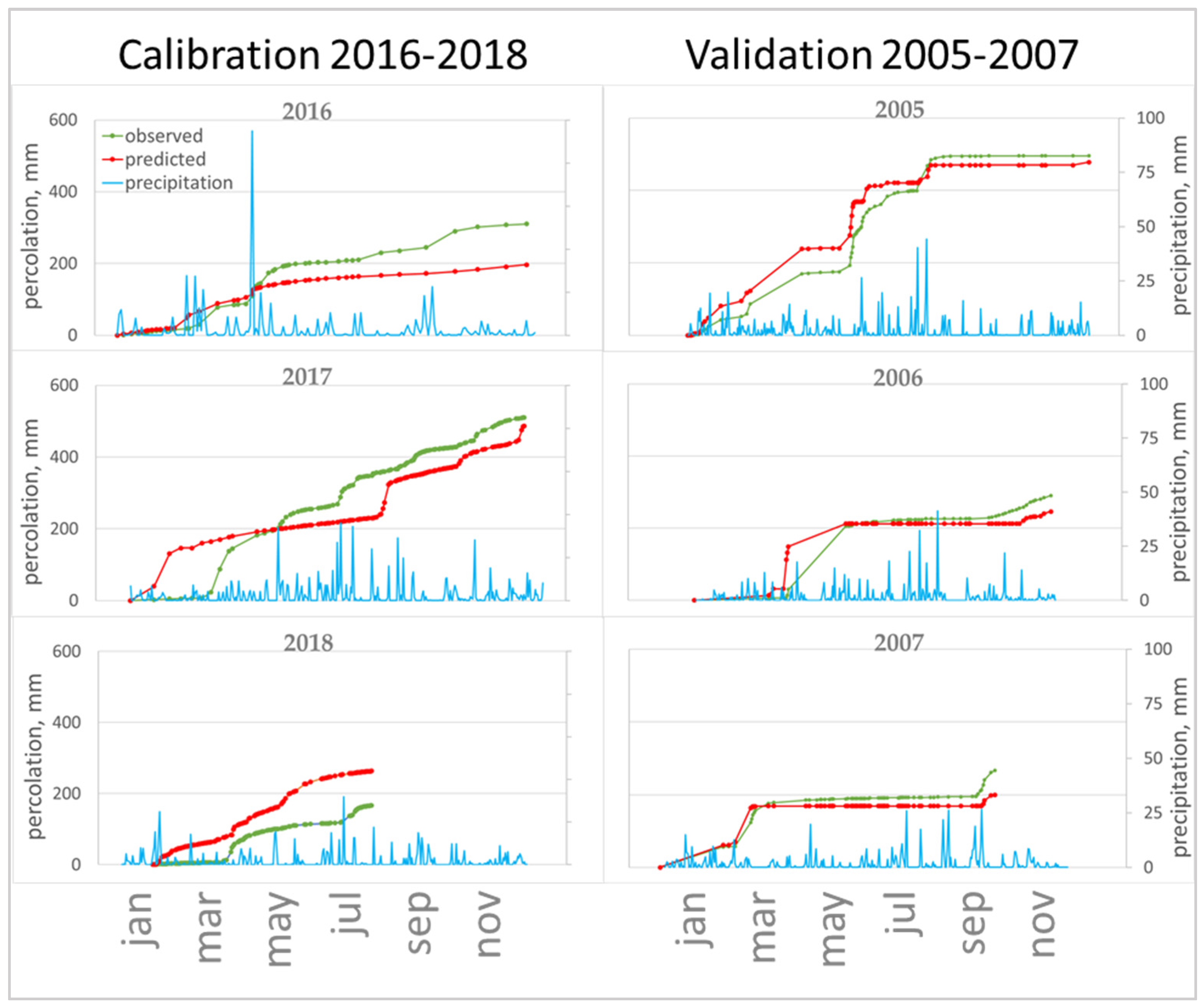
The final calibrating for the period from 10.06.2016 to 7.06.2017 is reflected in Table 5 (weather condition) and 6 (calibrated parameters and statistics) and will be called set2016 further in the text. The model has been verified with set2016 for the period 2016–2018 years. The overall result was less convincing; the total cumulative percolation forecast error was accumulated after each season (Figure 3), but by the end of the three-year period, the observed curve and the predicted curve practically converge. Therefore, the forecast quality was assessed for the period as a whole (EF 0.887, SRMSE 0.135) and for each year separately (2016: EF 0.747, SRMSE 0.37; 2017: EF 0.768, SRMSE 0.169; 2018: EF 0, −1.906, SRMSE 1.151). An assessment of the overall prediction of cumulative percolation, calculated for each year separately, indicates that the calibration did not give the desired result only for 2018. Analysis of differential curves points to weaknesses in the modelling: overestimation of cumulative percolation by the model in winter, underestimation of cumulative percolation during the period of active snowmelt in spring, discrepancy between the observed curve and the predicted curve in the summer-autumn period of alternating dry days and heavy precipitation.
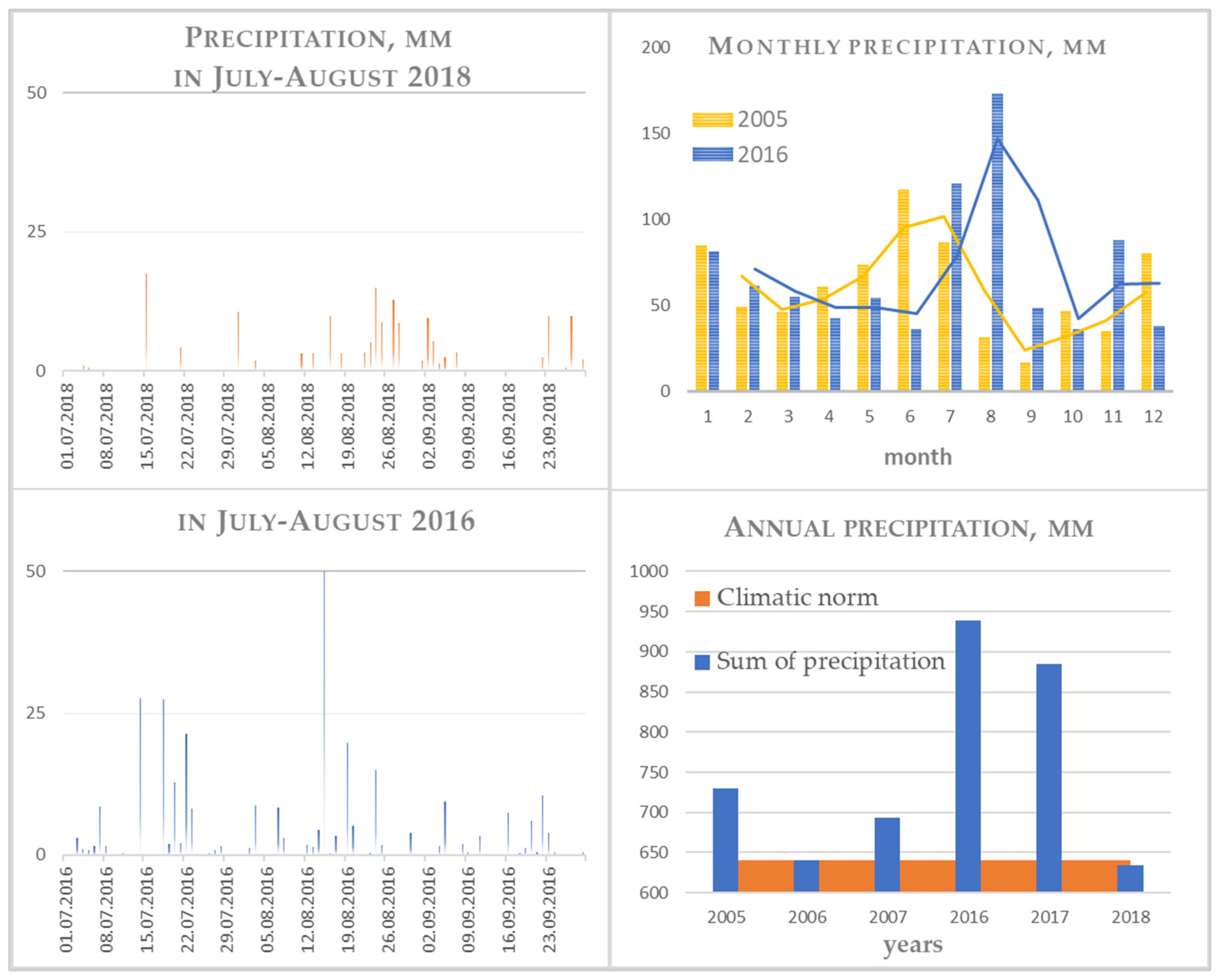
Table 5.
Weather conditions for two periods of simulation.
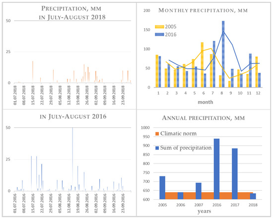
Figure 3.
Precipitation for the observation period.
In view of the weather features of the three-year period (2016–2018), it was decided to evaluate the validation for another time period (2005–2007), assuming that it would be possible to obtain averaged input parameters that will reduce the prediction errors for each of the years. However, this led to very ambiguous results, which, in our opinion, are related to intrasoil causes and conditions at the upper boundary and will be discussed below.
One of the best setting options for the period 2016–2018 (set2016) during validation for the period 2005–2007 showed an extremely high error in calculating the cumulative and diffusion percolation (Table 6). Thus, the calibrating even for the three-year period turned out to be unsuccessful when validating was carried out over a large time period. At the same time, a very unfortunate calibrating using pedotransfer functions (setPTF) during validation for the three-year period 2005–2007 unexpectedly showed an excellent result both in general and for individual years (2005–2007: EF 0.976, SRMSE 0.071) (Table 6), as well as the initial input set of soil parameters based on laboratory values of soil properties (setSoilLab).
Table 6.
Soil parameter sets for calibration and goodness-of-fit criteria.
Visual and statistical evaluation of the calibration results and the final prediction made it possible to conclude that the cumulative and differential percolation from the bottom of the soil is closely correlated not only with the total amount, but also with the intensity and frequency of precipitation at the upper boundary of the soil profile.
Weather conditions for two periods 2005–2007 and 2016–2018 are represented in Table 5 and Figure 3. In order to calculate the cumulative frequency distribution for annual rainfall, a dynamic model was used for a 20-year period (2000–2020). According to the amount of precipitation, the years used to work with the model were arranged as follows: a year of extremely low abundance (2%)—2016, a year of low abundance (10%)—2017, moderately abundant years (below 50%)—2005 and 2006, and the abundance of higher than medium (above 50%)—2018. It should be noted that for 2016, an especially great amount of precipitation fell in August; it was 1.5 times higher than the rainy months in other years, and half of them fell on the same day (24 August). It should also be noted that the feature of the distribution of precipitation throughout the year is as follows: comparison of July–September 2016 and 2018 in Figure 2. In 2018, against the background of a general low amount of precipitation, it was extremely unevenly distributed: the number of days without precipitation in August 2018 is 21, and 14 in August 2016, while precipitation of various intensity was observed and light rains up to 1 mm, and heavy rainfall of 30 mm or more, were observed.
In terms of the sum of active temperatures (>10 °C), 2017 is revealed as the coldest, and 2008 and 2018 as the warmest years with a long growing season. The hydrothermal coefficient [44], which is an easier-to-calculate analogue of the standardized SPI precipitation index that appeared much later, taking into account the sum of average daily temperatures for warm months for the period between the dates of temperature transition through 10 °C, reduced by 10 times, and the corresponding amount of precipitation, was used to characterize the maximum possible evaporation under existing atmospheric conditions.
where T > 10 °C is the sum of the average daily air temperatures for the period with air temperatures above 10 °C, P is the amount of precipitation for the same period. A value below or close to 1 allows us to classify 2018 as a moderately dry year for plants (Table 5).
In order to find a balance between model calibration and model validation of the corresponding set of input soil parameters, we successively returned from the set2016 version to the original setPTF and setSoilLab versions. The result of this work was a set of model input data (setBalance), for which for all years, except for 2018, a sufficiently high prediction accuracy was obtained, and validation for the period 2005–2007 was also successful (2016–2018: EF 0.870, SRMSE 0.145; 2005–2007: EF 0.690, SRMSE 0.256). In the course of calibrating, the values of TPORV, XMPOR, and KSATMIN are increased (Table 6).
3.2. Migration of Cyantraniliprole in the Experiment
Studies of cyantraniliprole leaching have been conducted since 2015. The first detection of cyantraniliprole in the percolation was observed on 22 June 2015, on the 8th day after application. The concentration of the pesticide in the water was 1.4 µg/L. During this period, 40 mm of precipitation fell. Such a rapid migration of the pesticide with the water flow firstly indicates transport through macropores, and, secondly, it is consistent with the data of other researchers. For instance, similar results were obtained in undisturbed lysimeters conducted by Beulk et al. [45]. The authors report that the maximum concentration of isoproturon—17.2 μg/L was observed in the period 20–40 days after application. In addition, a rapid breakthrough of isoproturon in the period 6–15 days after application was also observed by Nolan et al. [22]. July 2015 was rainy; in total, from the moment of processing until the end of July, 199 mm of precipitation fell. During this period, cyantraniliprole was found in all selected samples of lysimetric water in the concentration range of 1–2.8 µg/L. August was moderate in terms of precipitation; however, at the end of August, 47 mm of precipitation fell in 6 days, and on 29 August, and 31 August, concentrations of 12.5 and 10.8 µg/L, respectively, were recorded in the samples. In the autumn and early winter of 2015, cyantraniliprole was found in most samples; its concentration did not exceed 1 µg/L.
The subsequent water sampling was not carried out in winter. No cyantraniliprole was detected in the sample dated April 1, 2016. In June, prior to the next application, the concentration of cyantraniliprole was 0.7 µg/L. June was precipitation-poor (37 mm), while July (199 mm) and August (267 mm) were very rainy. At the same time, the insecticide was found in almost all water samples (with the exception of one), and the concentrations were in the range from 0.7 to 2.6 µg/L. Further, in the autumn and winter of 2016, as well as in 2017 and 2018, cyantraniliprole was found in most water samples at moderate concentrations up to 2.5 μg/L. There were three episodes with concentrations in the amount above 3 µg/L in October 2016, April and June 2017. During these periods, there was no significant amount of precipitation; in April, the substance leaching may have been connected with snowmelt. It is important to emphasize that cyantraniliprole was applied to the soil in 2015 and 2016; however, it was found in the cumulative percolation throughout the entire observation period, until the autumn of 2018.
Soil samples were taken to a depth of 50 cm. A year after the first treatment (June 2016), cyantraniliprole was distributed in a layer of 0–40 cm, and significant amounts were in layers up to 25 cm. In autumn 2016, the pesticide was detected in layers up to 50 cm, and up to 35 cm in May 2017.
3.3. Modelling Cyantraniliprole Migration
The initial input parameters of the rate of transformation and sorption of the pesticide and the range of their changes during the calibrating process are given in the table. Calculation with experimentally obtained parameters of sorption (Kos = 387, 1/n = 1) and transformation (DT50 = 49.9 days) [33,46], and with the best cumulative percolation calibrating (setBalance) showed that the model underestimates the cyantraniliprole residual in the soil. An increase in the value of the half-life time to 60 days made it possible to increase the accuracy of predicting the total amount of the pesticide in the soil and its distribution in the profile (input parameters and goodness-of-fit criteria are presented in Table 7, Table 8 and Table 9, distribution graphs in Figure 4). When calibrating the sorption coefficient, we focused on the distribution of cyantraniliprole in the soil profile, as well as on the flow out of the pesticide.
Table 7.
The initial input parameters of pesticide and the range of changes during calibration (in brackets).
Table 8.
Parameters changed during pesticide model calibration.
Table 9.
Goodness-of-fit criteria of accordance between observed and predicted cyantraniliprole concentration in the soil profile and in the leachate.
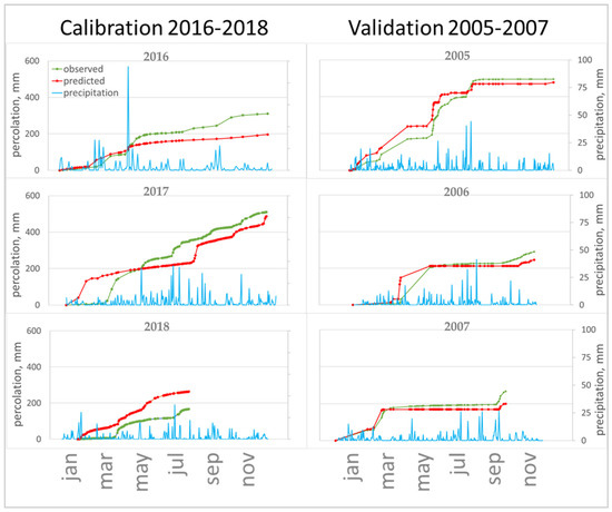
Figure 4.
Observed and predicted percolation, precipitation for calibrated and validated period.
At the initial input parameters, the model underestimated the depth of pesticide migration in the profile and did not predict its removal in the first two months after application (var. 1, Table 8). With a decrease in Koc setting in the upper horizons to 300, an increase in the accuracy of predicting concentrations in the profile was observed; nevertheless, the leaching of substance in the summer–autumn of 2015 was not predicted.
A decrease in the sorption coefficient led to a deterioration in the accuracy of estimating the distribution in the soil; at the same time, it did not lead to an improvement in the forecast of concentrations in the cumulative percolation; in particular, it did not allow to simulate the breakthrough of the pesticide in the summer of 2015. Therefore, it was decided to leave the sorption coefficient unchanged and adjust it by changing the dispersivity (DV) parameter, as well as increasing the ASCALE value in the lower horizons. Previously, in our studies [32,33], it has been found that the dispersion length parameter varies in soils within a significant range, and in clay soils, its value can reach 60 cm. An increase in the dispersion length parameter in the PEARL model led to an acceleration leaching of the pesticide from the soil. An increase in the dispersivity parameter to 50 cm slightly raised the accuracy of modelling the distribution of cyantraniliprole in the soil (Table 9); this led to the forecast of pesticide leaching in September 2015, but at a concentration lower than in the experiment. The subsequent calibrating was aimed at reducing the sorption coefficient in layers below 80 cm (Table 9.) and, at the same time, increasing the rate of transformation of cyantraniliprole in these horizons (layers). Thus, it was planned to achieve an increase in the leaching of the pesticide in the summer of 2015, but to reduce concentrations in the cumulative percolation in the subsequent period. The results achieved are reflected in the graphs (Figure 5 and Figure 6) and the measures of goodness-of-fit criteria of Table 9.
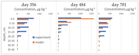
Figure 5.
Measured and simulated cyantraniliprole distributions on different sampling days in the lysimeter.
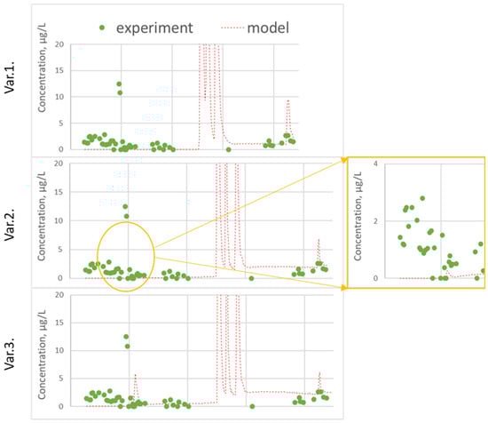
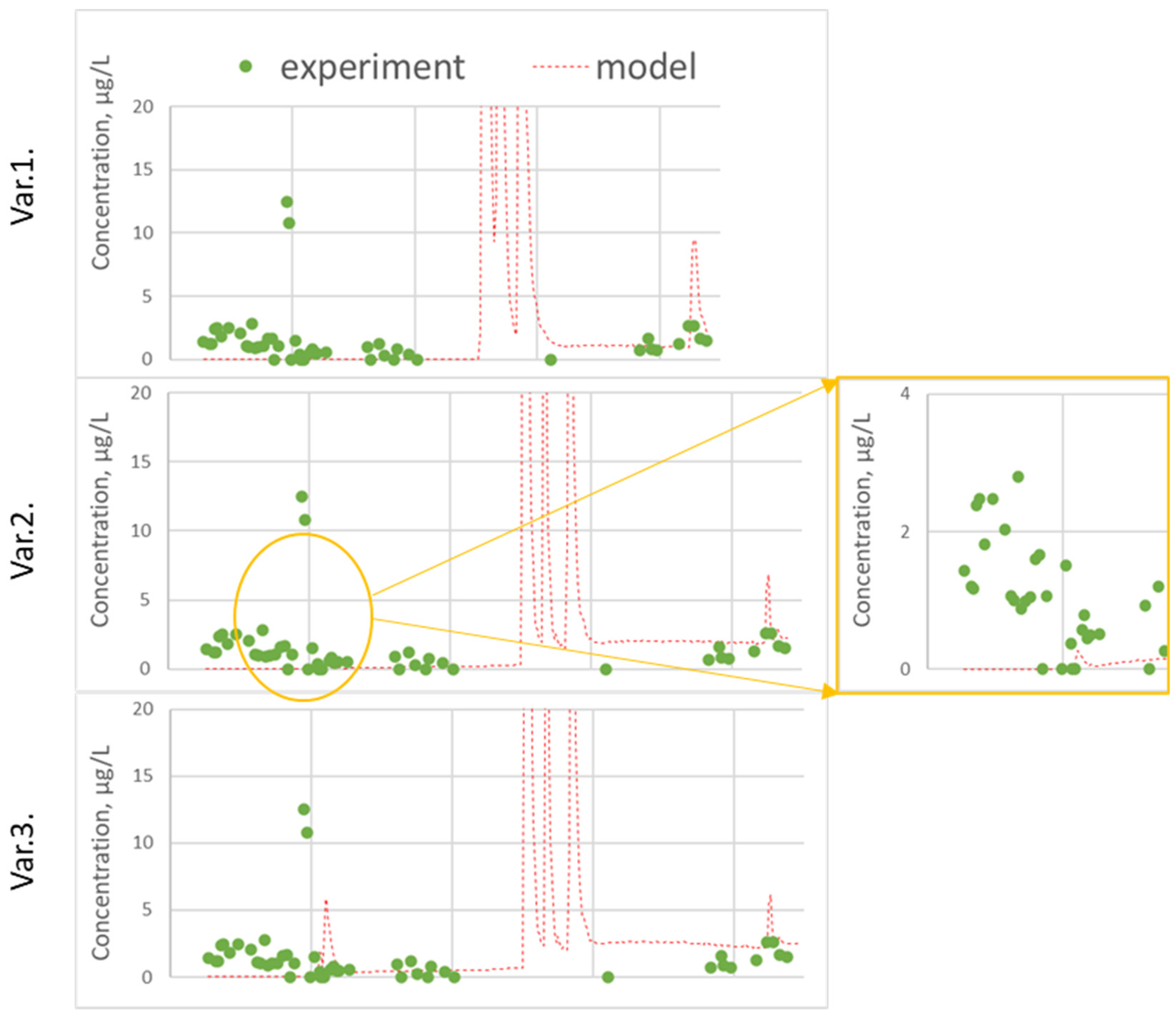
Figure 6.
Measured and predicted cyantraniliprole concentration in leachate: (var. 1) without calibration; (var. 2) DT50 and DV calibration; (var. 3) variant 2 + ASCALE, DT50 and Koc in deep horizons.
An assessment of the correlation between the predicted and experimental concentrations of cyantraniliprole in the percolate showed that satisfactory measures of goodness-of-fit criteria were obtained for the period from the application (June 2015) to August 2016, and satisfactory goodness-of-fit indicators were obtained (EF = 0.59 without calibration and EF = 0.47 var. 3).
In the time following, the model predicts two peaks of substance leaching in August 2016 and then in the spring of 2017, which are not confirmed experimentally. This is linked to poor forecast accuracy metrics (for the whole period of observation EF = 716.4 without calibration and EF = 14.6 var. 3).
As a result of calibrating, the accuracy of the prediction as a whole was improved; the peak of cyantraniliprole was predicted in September 2015, the observed values and predicted values of the center of mass, mean, median values and 80% percentile concentrations in the percolate converged.
In addition to the profile distribution of the pesticide, the concentrations of cyantraniliprole in the percolate were taken into account during calibrating. As noted above, in the experiment, an early leaching of cyantraniliprole was observed on the 8th day after application. None of the settings made it possible to achieve the appearance of the substance in water flow out of the bottom during this period. However, a large amount of precipitation in the second half of summer led to the leaching of cyantraniliprole, the concentration in the experiment at the end of August was about 10 µg/L.
The calculation with an increase in DT50 to 60 days, as well as the initial (experimentally determined) value of Koc, successfully predicted this peak; it appeared 2 weeks later (in mid-September), and the predicted concentration was 20 µg/L, which is two times more than in the experiment. Variation of the dispersivity led to the fact that the predicted leaching of the pesticide was not so sharp, the peak time did not change, and its value coincided with the experimental one. Measures of goodness for the period from 22.06.2015 to 6.08.2016 are represented in table. Thus, model calibration required a slight change in the input data, namely, an increase in the half-life time from 49.9 to 60 days and an increase in the dispersivity.
In the summer of 2016, the model also predicted a sharp peak of cyantraniliprole with a concentration more than 100 µg/L, which was not confirmed by experimental data. Perhaps this is due to the irregular sampling of water samples. In the container intended for collection, averaging took place over several days, which could to some extent smooth out the peak of the substance, naturally increasing the systematic error of the prediction.
4. Discussion
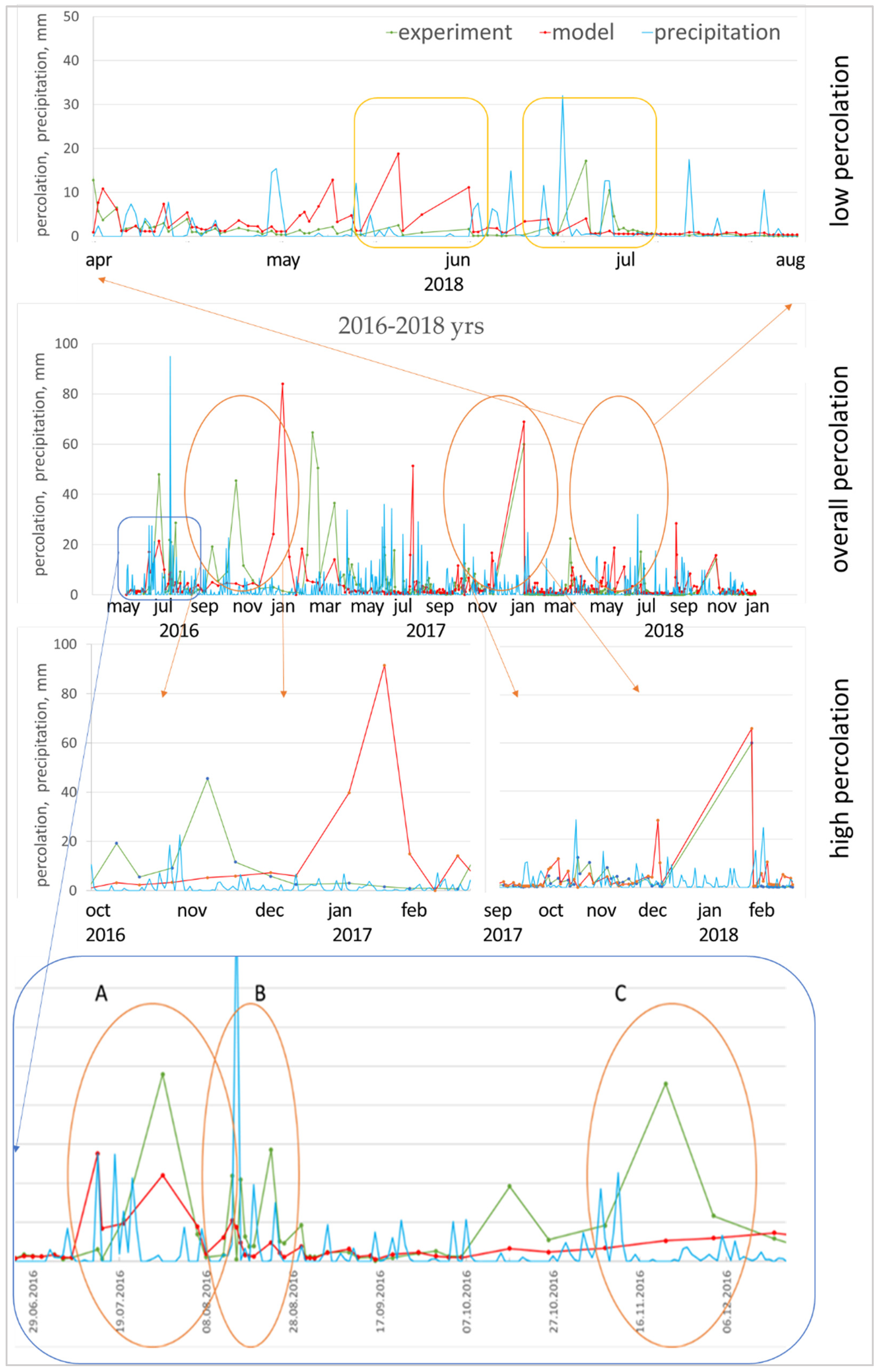
The manipulation result was achieved in two ways: (1) calibration for one year and verification for the next two years, (2) calibration for three years and verification for three years of a ten-year-old study. The result showed the significance of the meteorological parameters used in calibrating. The calibrating for 2016 was initially a poor decision, forasmuch as this year was characterized by a large amount of prolonged precipitation. In the course of registering the lysimetric cumulative percolation, it was noted that especially heavy precipitation was dispersed during the day, and therefore did not create excessive pressure head on the soil surface during infiltration (Figure 7B). On the other hand, quite a large number of days were accompanied by fast, but powerful showers (Figure 7A); during these periods, the limiting predictive cumulative percolation parameter will be the filtration rate of the upper horizon (KSM). Along with this, the cumulative percolation at the lower boundary of the lysimeter quite unambiguously reacts to the daily intensity of precipitation. The model flattens the curve of the cumulative percolation, producing few excess peaks during heavy precipitation (Figure 7A) and underestimating peaks during heavy but slow rainfall (Figure 7B). Another serious source of error is periods with several dry days after intense rainfalls, which end again with precipitation (Figure 7C), when macropores in the upper soil horizon make a large contribution to the total cumulative percolation from the lower boundary.
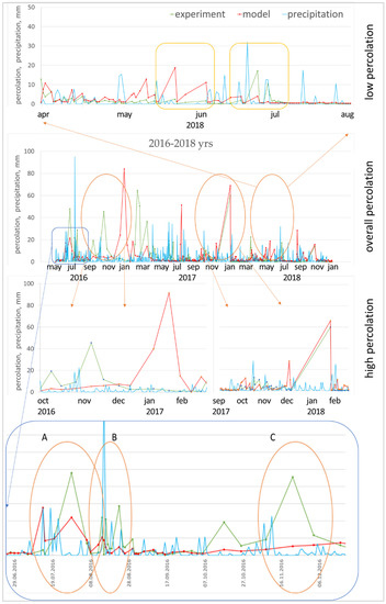
Figure 7.
Measured and predicted percolation in different periods of the study: (A) several excess peaks during heavy precipitation; (B) underestimation of percolation peaks during heavy but slow rains; (C) periods with several dry days after intense rainfall, which again end in precipitation.
The year 2018 (Figure 7) is especially indicative in terms of precipitation (low percolation period). In July, the model significantly overestimated the cumulative percolation against the background of dry days ending in intense precipitation; on the other hand, it underestimated the cumulative percolation in July, when heavy and frequent precipitation was observed.
In snowmelt, it has been established that the migration ability of various elements in the soil is determined not only by the sorption properties of soils and the amount of precipitation, but also by the form of water migration in the profile. It has been revealed that during heavy rainfall preceded by dry periods and during periods of intense melting water transfer, conditions are formed for the rapid release of gravitational water and the transit of substances with preferential flows.
This leads to the conclusion that in order to conduct the calibrating of the water migration models, long periods with different precipitation availability, different intensity of precipitation during the season are necessary, and even the daily dynamics of precipitation have a significant impact on calibrating. Taking into account that when solving applied problems, such as assessing the risk of pesticides leaching from the soil profile during their state registration, ten-year and longer time periods are used, then small differential cumulative percolation errors similar to those described can either be compensated or accumulated, enhancing the systematic component of the model forecast error. The use of long time intervals for calibrating, selected taking into account the variety of rainfall conditions, will lead to a more stable prediction result in the future.
However, if we take a long period for calibrating (2015–2017), then the calibrating does not lead to an equally successful result for all years (the same error in trend and value). In this case, it is necessary to consider the soil itself, with the soil hydraulic properties of which, when modelling, we are trying to reconstruct its pore space, to describe the water flow as accurately as possible during precipitation of different intensity.
In reality, when the soil experiences waterlogging, swelling processes are taking place. Its pore space has a different geometry (tortuosity and pore volume change) than dry soil, where cracks form and small pores open [41]. At this stage of the development of the mathematical modelling method, it is impossible to state with certainty that the model is able to successfully describe this difference in two soil conditions. It turns out that in order to correctly reflect the real pattern of water flows distribution in the soil profile two or more sets of soil parameters (primarily those responsible for the pore space) are required. Additionally, each set of soil parameters to calibrating should be used in “its ideal period”. This is what happened when the ideal set of soil properties was selected for 2016; however, “it did not work” for 2018, when the soil most likely became more cracked in the humus horizon, and the main water volume was stored in the middle part of the profile, and then appeared at the bottom in large portions. Therefore, when using one set of soil properties, it was necessary to find a balance using soil physical parameters between soil conditions in different rainfall conditions. This explains the fact that the parameters most influencing the predicted cumulative percolation during calibrating were soil porosity, macropore volume and filtration rate in soil matrix.
However, the question arises why the quality of the forecast during model verification was consistently lower than the result of the forecast during setting. This is not connected with short-term and practically reversible changes in the pore space, but it is connected with slow evolutionary processes occurring in the soil profile, which are also based on differences in the transit properties of the soil during periods of uneven precipitation. With a gradual frontal water migration, the mobility of a number of elements increases and processes of intense intrasoil weathering occur (in situ). Previous scientific works in the field of evolution of lysimetric soils showed a pronounced transformation of the solid phase of lysimeter soils and a change in soil structure towards a cloddy, and for the lower horizons, a blocky structure [37,47]. The soil density also gradually increases. First of all, the process of soil transformation in lysimeters is connected with the removal of silt fractions into the underlying horizons and their leaching. This explains, among other things, an increase in the content of organic matter in horizon B3.
Calibration the model according to the profile distribution of the pesticide and the concentrations of the pesticide in the water flow from the lower boundary demanded changing the half-life period from 49.9 to 60 days in the 0–40 cm layer and up to 120 days in the 40–150 cm layer. In all layers, the sorption coefficient was lowered by 1.3 times, and in the 60–80 cm layer, it was reduced by a factor of 2.3. Changes in the decomposition rate and sorption coefficient in the deep layers made it possible to conduct fine setting, by reducing the sorption coefficient, achieving a faster leaching of the pesticide, and by reducing the transformation rate in the lower layers, achieving a decrease in the predicted concentrations in the long term.
The research has established that the model is highly sensitive to the dispersivity and ASCALE parameters, the values of which can be a convenient tool when calibrating the model. The ASCALE parameter controls the exchange of water and solutions between micro- and macropores; it increases in soils that have a high percentage of clay, and it increases with depth in silty clays and clays. An increase in DV (dispersivity) leads to an increase in the leaching front in the soil matrix; thus, it leads to a reduction in the availability of the pesticide for the preferred migration flow in structured silty clayey soils, reducing the removal of the pesticide. Thus, by reducing sorption in the soil, we achieve rapid migration of the pesticide and an increase in its concentration in the percolate after 1 year and later. By increasing the ASCALE and DV parameters, we limit the fast transport in the long run. Thus, the simultaneous variation of Koc, DV and ASCALE allows conducting finer calibration of the movement of pesticides in the soil.
Despite the fact that the MACRO 5.2 model describes the transport of substances through macropores, and it was carefully parameterized and calibrated against water flow out of the bottom of the profile, it was nevertheless not possible to predict the early pesticide leaching on 8 days after application. The calibrating made it possible to predict the leaching on 1.5 months after application. However, the obvious result of the research is the fact that pesticide calibration did not significantly improve the accuracy of the prediction. Some improvement in the statistical parameters of correspondence and convergence of predicted and observed mean, median and 80% percentile pesticide concentrations in the percolate has been achieved.
5. Conclusions
In the course of applying careful parameterization of the MACRO 5.2 model based on experimental studies of input parameters and expert evaluation of difficult-to-determine parameters, the water flow prediction from the lower boundary of the Albic Glossic Retisol of lysimeters is unsatisfactory, and the model needs additional calibration of the input data. The calibration mainly concerns those parameters to which the model is most sensitive, namely, the parameters that determine the pore space structure. However, there are no specific guidelines on how to carry out calibration and validation model.
When choosing a calibration period, it is necessary to take into account the conditions at the upper boundary, choosing, if possible, large intervals for calibration and validation model. In this case, the source of systematic errors, along with the upper boundary condition, will be the transformation of the pore space structure of the soil in daily, seasonal and annual cycles, as well as a result of global evolutionary processes in soils.
Comparison of experimental and predicted concentrations in soil and percolate of the moderately mobile and moderately resistant insecticide cyantraniliprole showed that the ability of the model to predict its migration in silt loam soil was found to be poor. The accuracy of predicting to measures of goodness-of-fit criteria increased when the parameters of pesticide transformation, as well as parameters of soil dispersion and water flow and solutions between micro- and macropores, were calibrated. However, increasing the pesticide’s speed of movement in the early period resulted in the excess of projected concentrations in a year and later, and changing average concentration values over a lengthy period of time reduced the removal in the initial time after application.
In order to solve some applied problems (risk assessment of pesticide leaching from the soil during the state registration of new active substances of pesticides), model calibrating by setting parameters is a tool that makes it possible to adjust the volume of percolate. Along with this, due to the fact that the migration of pesticides in the soil occurs mainly with water flows, the qualitative calibration of the water part of the model is the key to the accurate prediction of the migration of substances in the soil profile. However, for the purposes of developing the method of mathematical modelling, the determination of experimental soil properties is a necessary step for understanding the direction and essence of those soil processes, which occur not only in the topsoil, but also in the underlying horizons (which have different properties as described using the genetic approach of the soil science founder V.V. Dokuchaev), which was clearly demonstrated by the calibration of the pesticide part of the model.
Author Contributions
Conceptualization, V.K. and A.K.; methodology, V.K. and A.K.; software, A.K. and A.B. (Alexandra Belik), validation, V.K., A.K. and A.B. (Alexandra Belik); formal analysis, A.G. and A.B. (Andrei Bolotov); investigation, A.K., V.K. and A.B. (Alexandra Belik); resources, V.K. and A.K.; data curation, V.K.; writing—original draft preparation, V.K., A.K. and A.B. (Alexandra Belik); writing—review and editing, V.K. and A.K.; visualization, V.K., A.K. and A.B. (Alexandra Belik); supervision, V.K.; project administration, V.K. and A.K.; funding acquisition, A.B. (Andrei Bolotov). All authors have read and agreed to the published version of the manuscript.
Funding
This research received no external funding.
Informed Consent Statement
Not applicable.
Data Availability Statement
Not applicable.
Acknowledgments
This study was supported by the State Project of Russian Scientific—Research Institute of Phytopathology No. 0598-2019-0005 (statement of the problem, conceptual generalization, pesticide analysis), by the Russian Federation for Basic Research, projects N 19-29-05252 (object), projects N 20-05-00773 (meteorological observations). Additionally, the research was carried out within the state assignment of Ministry of Science and Higher Education of the Russian Federation (theme No. 121040800146-3 “Physical bases of ecological functions of soils: technologies of monitoring, forecasting and management”) (soil analysis).
Conflicts of Interest
The authors declare no conflict of interest.
References
- Blanchoud, H.; Farrugia, F.; Mouchel, J.M. Pesticide Uses and Transfers in Urbanised Catchments. Chemosphere 2004, 55, 905–913. [Google Scholar] [CrossRef] [PubMed]
- Hildebrandt, A.; Guillamón, M.; Lacorte, S.; Tauler, R.; Barceló, D. Impact of Pesticides Used in Agriculture and Vineyards to Surface and Groundwater Quality (North Spain). Water Res. 2008, 42, 3315–3326. [Google Scholar] [CrossRef] [PubMed]
- Herrero-Hernández, E.; Andrades, M.; Alvarez-Martin, A.; Pose-Juan, E.; Rodríguez-Cruz, M.S.; Sánchez-Martín, M. Occurrence of Pesticides and Some of Their Degradation Products in Waters in a Spanish Wine Region. J. Hydrol. 2013, 486, 234–245. [Google Scholar] [CrossRef]
- Vega, A.; Frenich, A.; Vidal, J. Monitoring of Pesticides in Agricultural Water and Soil Samples from Andalusia by Liquid Chromatography Coupled to Mass Spectrometry. Anal. Chim. Acta 2005, 538, 117–127. [Google Scholar] [CrossRef]
- Carter, A.D. Herbicide Movement in Soils: Principles, Pathways and Processes. Weed Res. 2000, 40, 113–122. [Google Scholar] [CrossRef]
- FOCUS (FOrum for Co-Ordination of Pesticide Fate Models and Their Use). FOCUS Groundwater Scenarios in the EU Review of Active Substances: Report of the FOCUS Groundwater Scenarios Workgroup EC Document Reference Sanco/321/ 2000 Rev.2. 2000; 202p. Available online: https://esdac.jrc.ec.europa.eu/public_path/projects_data/focus/gw/docs/FOCUS_GW_Report_Main.pdf (accessed on 24 February 2022).
- Larsbo, M.; Jarvis, N. MACRO 5.0: A Model of Water Flow and Solute Transport in Macroporous Soil, Technical Description. Available online: https://www.yumpu.com/en/document/view/28675249/users-guide-to-macro50-a-model-of-water-flow-and-solute (accessed on 24 February 2022).
- Leistra, M.; van der Linden, A.M.A.; Boesten, J.; Tiktak, A.; van der Berg, F. PEARL Model for Pesticide Behaviour and Emissions in Soil-Plant Systems; Description of the Processes in FOCUS PEARL v 1.1.1; Wageningen Environmental Research: Wageningen, The Netherlands, 2001; p. 115. [Google Scholar]
- Klein, M. PELMO Pesticide Leaching Model, Version 2.01, User’s Manual; Fraunhofer-Institut fur Umweltchemie und Okotoxikolgie: Schmallenberg, Germany, 1995. [Google Scholar]
- Carsel, R.; Imhoff, J.; Hummel, P.; Cheplick, J.; Donigian, A.; Suarez, L. PRZM-3, a Model for Predicting Pesticide and Nitrogen Fate in the Crop Root and Unsaturated Soil Zones: User’s Manual for Release 3.12.2; US Environmental Protection Agency (EPA): Washington, DC, USA, 2005.
- Vanclooster, M.; Boesten, J.; Trevisan, M.; Brown, C.; Capri, E.; Eklo, O.; Gottesbüren, B.; Gouy, V.; Linden, A.M.A. A European Test of Pesticide-Leaching Models: Methodology and Major Recommendations. Agric. Water Manag. 2000, 44, 1–19. [Google Scholar] [CrossRef]
- Scorza, R., Jr.; Boesten, J. Simulation of Pesticide Leaching in a Cracking Clay Soil with the PEARL Model. Pest Manag. Sci. 2005, 61, 432–448. [Google Scholar] [CrossRef]
- Kolupaeva, V.; Gorbatov, V.; Kokoreva, A. Comparison of PEARL and MACRO_DB Simulations in the Unsaturated Zone Using Lysimeter Experiment Data. In Environmental Fate and Ecological Effects of Pesticides; Re, A.A.M.D., Capri, E., Fragoulis, G., Trevisan, M., Eds.; La Goliardica Pavese s.r.l.: Pavia, Italy, 2007; pp. 497–502. [Google Scholar]
- Shein, E.; Belik, A.; Kokoreva, A.; Kolupaeva, V. Quantitative Estimate of the Heterogeneity of Solute Fluxes Using the Dispersivity Length for Mathematical Models of Pesticide Migration in Soils. Eurasian Soil Sci. 2018, 51, 797–802. [Google Scholar] [CrossRef]
- Zappa, G.; Bersezio, R.; Felletti, F.; Giudici, M. Modeling Heterogeneity of Gravel-Sand, Braided Stream, Alluvial Aquifers at the Facies Scale. J. Hydrol. 2006, 325, 134–153. [Google Scholar] [CrossRef]
- Vassena, C.; Cattaneo, L.; Giudici, M. Assessment of the Role of Facies Heterogeneity at the Fine Scale by Numerical Transport Experiments and Connectivity Indicators. Appl. Hydrogeol. 2010, 18, 651–668. [Google Scholar] [CrossRef]
- Šimůnek, J.; Jarvis, N.; Genuchten, M.V.; Gärdenäs, A.I. Review and Comparison of Models for Describing Non-Equilibrium and Preferential Flow and Transport in the Vadose Zone. J. Hydrol. 2003, 272, 14–35. [Google Scholar] [CrossRef]
- Dubus, I.G.; Beulke, S.; Brown, C.D.; Gottesbüren, B.; Dieses, A. Inverse Modelling for Estimating Sorption and Degradation Parameters for Pesticides. Pest Manag. Sci. 2004, 60, 859–874. [Google Scholar] [CrossRef] [PubMed]
- Beulke, S.; Dubus, I.; Brown, C.; Gottesbüren, B. Simulation of Pesticide Persistence in the Field on the Basis of Laboratory Data—A Review. J. Environ. Qual. 2000, 29, 1371–1379. [Google Scholar] [CrossRef]
- Vereecken, H.; Vanderborght, J.; Kasteel, R.; Spiteller, M.; Schäffer, A.; Close, M. Do Lab-Derived Distribution Coefficient Values of Pesticides Match Distribution Coefficient Values Determined from Column and Field-Scale Experiments? A Critical Analysis of Relevant Literature. J. Environ. Qual. 2011, 40, 879–898. [Google Scholar] [CrossRef]
- Scorza, R.P., Jr.; Jarvis, N.J.; Boesten, J.J.; van der Zee, S.E.; Roulier, S. Testing MACRO (Version 5.1) for Pesticide Leaching in a Dutch Clay Soil. Pest Manag. Sci. 2007, 63, 1011–1025. [Google Scholar] [CrossRef] [Green Version]
- Nolan, B.T.; Dubus, I.G.; Surdyk, N. A Refined Lack-of-Fit Statistic to Calibrate Pesticide Fate Models for Responsive Systems. Pest Manag. Sci. 2009, 65, 1367–1377. [Google Scholar] [CrossRef]
- Marín-Benito, J.M.; Pot, V.; Alletto, L.; Mamy, L.; Bedos, C.; Barriuso, E.; Benoit, P. Comparison of Three Pesticide Fate Models with Respect to the Leaching of Two Herbicides under Field Conditions in an Irrigated Maize Cropping System. Sci. Total Environ. 2014, 499, 533–545. [Google Scholar] [CrossRef]
- Shein, E.; Kokoreva, A.; Gorbatov, V.; Umarova, A.; Kolupaeva, V.; Perevertin, K.A. Sensitivity Assessment, Adjustment, and Comparison of Mathematical Models Describing the Migration of Pesticides in Soil Using Lysimetric Data. Eurasian Soil Sci. 2009, 42, 769–777. [Google Scholar] [CrossRef]
- Marín-Benito, J.; Mamy, L.; Carpio, M.; Sánchez-Martín, M.; Rodriguez-Cruz, S. Modelling Herbicides Mobility in Amended Soils: Calibration and Test of PRZM and MACRO. Sci. Total Environ. 2020, 717, 137019. [Google Scholar] [CrossRef]
- Kolupaeva, V.N.; Gorbatov, V.S.; Shein, E.V.; Leonova, A.A. The Use of the PEARL Model for Assessing the Migration of Metribuzin in Soil. Eurasian Soil Sci. 2006, 39, 597–603. [Google Scholar] [CrossRef]
- Baratelli, F.; Giudici, M.; Vassena, C. Single and Dual-Domain Models to Evaluate the Effects of Preferential Flow Paths in Alluvial Sediments. Transp. Porous Media 2011, 87, 465–484. [Google Scholar] [CrossRef]
- Roulier, S.; Jarvis, N. Modeling Macropore Flow Effects on Pesticide Leaching: Inverse Parameter Estimation Using Microlysimeters. J. Environ. Qual. 2003, 32, 2341–2353. [Google Scholar] [CrossRef] [PubMed] [Green Version]
- Jarvis, N.J. MACRO (V5.2): Model Use, Calibration, and Validation. Trans. ASABE 2012, 55, 1413–1423. [Google Scholar] [CrossRef]
- Jarvis, N.; Larsbo, M.; Roulier, S.; Lindahl, A.; Persson, L. The Role of Soil Properties in Regulating Non-Equilibrium Macropore Flow and Solute Transport in Agricultural Topsoils. Eur. J. Soil Sci. 2007, 58, 282–292. [Google Scholar] [CrossRef]
- PPDB—Pesticide Properties Database. Available online: https://sitem.herts.ac.uk/aeru/ppdb/en/ (accessed on 28 February 2022).
- Kolupaeva, V.; Kokoreva, A.; Belik, A.; Pletenev, P. Study of the Behavior of the New Insecticide Cyantraniliprole in Large Lysimeters of the Moscow State University. Open Agric. 2019, 4, 599–607. [Google Scholar] [CrossRef]
- Kolupaeva, V.; Nyukhina, I.; Belik, A. Study of Cyantraniliprole Sorption in Soils of Russia. E3S Web Conf. 2020, 169, 01022. [Google Scholar] [CrossRef]
- Larsbo, M.; Jarvis, N. Simulating Solute Transport in a Structured Field Soil. J. Environ. Qual. 2005, 34, 621–634. [Google Scholar] [CrossRef] [Green Version]
- Vanclooster, M.; Pineros-Garcet, J.D.; Boesten, J.J.T.I.; Van den Berg, F.; Leistra, M.; Smelt, J.H.; Jarvis, N.; Burauel, P.; Vereecken, H.; Wolters, A.; et al. APECOP: Effective Approaches for Assessing the Predicted Environmental Concentrations of Pesticides—Final Report; Department of Environmental Sciences and Land Use Planning, Université Catholique de Louvain: Wallonia, Belgium, 2003; p. 158. [Google Scholar]
- Beulke, S.; Brown, C.D.; Jarvis, N.J. Macro: A Preferential Flow Model to Simulate Pesticide Leaching and Movement to Drains. In Modelling of Environmental Chemical Exposure and Risk; Linders, J.B.H.J., Ed.; Springer: Dordrecht, The Netherlands, 2001; pp. 117–132. [Google Scholar] [CrossRef]
- Umarova, A.B.; Arkhangelskaya, T.A.; Kokoreva, A.A.; Ezhelev, Z.S.; Shnyrev, N.A.; Kolupaeva, V.N.; Ivanova, T.V.; Shishkin, K.V. Long-term research on physical properties of soils in the large lysimeters of Moscow State University: Main results for the first 60 years (1961–2021). Mosc. Univ. Soil Sci. Bull. 2021, 76, 95–110. [Google Scholar] [CrossRef]
- Beulke, S.; Renaud, F.; Brown, C. Development of Guidance on Parameter Estimation for the Preferential Flow Model MACRO 4.2. Available online: https://www.semanticscholar.org/paper/Development-of-guidance-on-parameter-estimation-for-Beulke-Renaud/f6ce86c308ca6a038891b277e913cddb332533a4 (accessed on 24 February 2022).
- Shein, E.V. Granulometric Composition of Soils: Problems of Research Methods, Interpretation of Results and Classifications. Soil Sci. 2009, 3, 309–317. [Google Scholar]
- Umarova, A.B. Preferention Flows in Soils: Patterns of Formation and Significance in the Functioning of Soils; GEOS: Moscow, Russia, 2011; p. 266. ISBN 978-5-89118-562-3. [Google Scholar]
- Belik, A.A.; Kokoreva, A.A.; Bolotov, A.G.; Dembovetskii, A.V.; Kolupaeva, V.N.; Korost, D.V.; Khomyak, A.N. Characterizing Macropore Structure of Agrosoddy-Podzolic Soil Using Computed Tomography. Open Agric. 2020, 5, 888–897. [Google Scholar] [CrossRef]
- Ritter, A.; Muñoz-Carpena, R. Performance Evaluation of Hydrological Models: Statistical Significance for Reducing Subjectivity in Goodness-of-Fit Assessments. J. Hydrol. 2013, 408, 33–45. [Google Scholar] [CrossRef]
- Dubus, I.G.; Brown, C.D.; Beulke, S. Sensitivity Analyses for Four Pesticide Leaching Models. Pest Manag. Sci. 2003, 59, 962–982. [Google Scholar] [CrossRef] [PubMed]
- Evarte-Bundere, G.; Evarts-Bunders, P. Using of the Hydrothermal Coefficient (Htc) for Interpretation of Distribution of Non-Native Tree Species in Latvia on Example of Cultivated Species of Genus TILIA. Acta Biol. Univ. Daugavp. 2012, 12, 135–148. [Google Scholar]
- Beulke, S.; Brown, C.; Dubus, I.; Fryer, C.; Walker, A. Evaluation of Probabilistic Modelling Approaches against Data on Leaching of Isoproturon through Undisturbed Lysimeters. Ecol. Model. 2004, 179, 131–144. [Google Scholar] [CrossRef] [Green Version]
- Kolupaeva, V.N.; Gorbatov, V.S.; Nuhina, I.V. Determination of Transformation Parameters of Cyantraniliprole in Soddy-Podzolic Soil in Laboratory Conditions. Bull. NGAU Novosib. State Agrar. Univ. 2016, 2, 82–91. [Google Scholar]
- Umarova, A.; Ivanova, T. Dynamics of the Dispersity of Model Soddy-Podzolic Soils in a Long-Term Lysimetric Experiment. Eurasian Soil Sci. 2008, 41, 519–528. [Google Scholar] [CrossRef]


Publisher’s Note: MDPI stays neutral with regard to jurisdictional claims in published maps and institutional affiliations. |
© 2022 by the authors. Licensee MDPI, Basel, Switzerland. This article is an open access article distributed under the terms and conditions of the Creative Commons Attribution (CC BY) license (https://creativecommons.org/licenses/by/4.0/).