Article

Development of Data-Driven Models to Predict Biogas Production from Spent Mushroom Compost

1
Department of Civil and Environmental Engineering, Prince of Songkla University, Hat Yai 90110, Thailand
2
Department of Civil Engineering, University of Manitoba, Winnipeg, MB R3T 5V6, Canada
3
PSU Energy Systems Research Institute, Prince of Songkla University, Hat Yai 90110, Thailand
*
Author to whom correspondence should be addressed.
Agriculture 2022, 12(8), 1090; https://doi.org/10.3390/agriculture12081090
Submission received: 21 June 2022 / Revised: 18 July 2022 / Accepted: 20 July 2022 / Published: 24 July 2022
(This article belongs to the Special Issue Modeling the Adaptations of Agricultural Production to Climate Change)

Abstract

:
In this study, two types of data-driven models were proposed to predict biogas production from anaerobic digestion of spent mushroom compost supplemented with wheat straw as a nutrient source. First, a k-nearest neighbours (k-NN) model (k = 1–10) was constructed. The optimal k value was determined using the cross-validation (CV) method. Second, a support vector machine (SVM) model was developed. The linear, quadratic, cubic, and Gaussian models were examined as kernel functions. The kernel scale was set to 6.93, while the box constraint (C) was optimized using the CV method. Results demonstrated that R2 for the k-NN model (k = 2) was 0.9830 at 35 °C and 0.9957 at 55 °C. The Gaussian-based SVM model (C = 1200) provided an R2 of 0.9973 at 35 °C and 0.9989 at 55 °C, which are slightly better than those achieved by k-NN. The Gaussian-based SVM model produced RMSE of 0.598 at 35 °C and 0.4183 at 55 °C, which are 58.4% and 49.5% smaller, respectively, than those produced by the k-NN. These findings imply that SVM modeling can be considered a robust technique in predicting biogas production from AD processes as they can be implemented without requiring prior knowledge of biogas production kinetics.

Graphical Abstract

1. Introduction

The electrical and thermal energy production processes that use non-renewable resources (i.e., fossil fuels; oil, and coal) are becoming less attractive globally. Even though such resources are rich in energy and relatively inexpensive to process, they are limited in supply and will soon be depleted. In addition, the utilization of fossil fuels emits additional greenhouse gases into the atmosphere, which has instigated climate change [1]. Hence, a large number of research bodies have aligned to overcome such an increasing universal concern. One of the most promising and attractive alternative solutions is the use of biogas derived from wastes or renewable feedstock [2,3].
Biogas, a mixture consisting chiefly of methane (CH4) and carbon dioxide (CO2), is the end-product of anaerobic digestion of organic matters (e.g., agricultural residues, livestock manure, food waste, sewage sludge, etc.) [4,5,6,7,8]. Anaerobic digestion is a complex multi-step process that is carried out by a consortium of different microbial species known as anaerobes. Uniquely, they do not need molecular oxygen for their metabolism and growth [9]. The key steps of the anaerobic digestion process, together with the possible applications of biogas, and its adverse environmental impacts are outlined in Figure 1.
The increasing global interest in biogas power plant establishment via anaerobic digestion of various organic matters has resulted in attempts to develop numerous mathematical models to predict and suggest optimal operations. Hill [15] developed a model to describe the digestion of animal wastes, assuming that the main five bacterial groups involved in the overall digestion process (acidogenic bacteria, hydrogenotrophic bacteria, homoacetogenic bacteria, acetoclastic bacteria, and H2 utilizing methane bacteria) are inhibited by a high concentration of fatty acids (FAs). Mosey [16] proposed a model consisting of four reactions (one acidogenic reaction, one acetogenic reaction, and two methanogenic reactions), which also takes into account the role of H2. According to this model, in case of a sudden rise in the organic loading rate, an accumulation of volatile fatty acids (VFAs) is likely to occur; this results in a decrease in pH that inhibits H2 utilizing methanogenic bacteria. In other words, H2 partial pressure is increased, which leads to further accumulation of propionic/butyric acid (CH4 generation is stopped when pH drops below 5.5). Based on Mosey’s model, Pullammanappallil et al. [17] introduced a model taking into account the gas phase, and acetoclastic inhibition by undissociated FAs. Angelidaki et al. [18] presented a model considering hydrolysis, acidogenesis, acetogenesis, and methanogenesis, which is suitable to describe the behavior of anaerobic digesters fed with manures. This model was developed by incorporating some assumptions as follows: (i) methanogenesis is inhibited by free NH3, (ii) acetogenesis is inhibited by acetic acid, (iii) acidogenesis is inhibited by total VFAs, and (iv) the degree of NH3 ionization, the maximum specific growth rate of bacteria are pH and temperature dependent.
In all the above-mentioned models, organic material was taken into account as a whole; in other words, they are incapable of dealing with complex feed composition. In this regard, the International Water Association (IWA) task group for mathematical modeling of the anaerobic digestion process developed a model known as Anaerobic Digester Model No 1 (more often abbreviated as ADM1), that takes the complex organic substrates into account [19].
Although the kinetic-based mathematical models for describing the anaerobic digestion process can help engineers and asset managers to better plan the management of the biogas plants, it is often criticized that most of them are inherently too complex due to a large number of stoichiometric coefficients and parameters reflecting the kinetic properties of the enzymes and microorganisms that govern the physicochemical and biochemical reactions through anaerobic digestion processes [20]. In addition, these models typically involve physicochemical equilibrium expressions and differential mass balance equations for components in the liquid phase (substrates for acidogenic/acetogenic/methanogenic organisms and their corresponding microbial masses) and in the gas phase (e.g., CH4 and CO2). Hence, these models are often complicated to solve, and many simplifying assumptions must be made to reduce their complexity. However, incorporating simplifying assumptions into the models may not hold in practice. Fedailaine et al. [21] modeled the biokinetics of the anaerobic digestion process involving eight simplifying assumptions, which inevitably limited the application of this model to full-scale anaerobic digesters. In addition, applying assumptions to the models lowers the precision of the models; in other words, an under- or over-estimation of the response of the models will likely occur. For these reasons, developing a simple yet highly predictive model to estimate biogas production from the anaerobic digestion process is highly desired. As such, a different branch of models, called artificial intelligence (AI)-based models (more often known as easy-to-use black-box models) may be recruited. These models have advantages over complex mathematical models because they are constructed on a measured dataset (i.e., input–output data pairs for a given system) without requiring complicated kinetic relationships between the input variables and the corresponding outputs [22,23]. In addition, the AI modeling approach is proven as a robust tool with high generalization power. Holubar et al. [24] used an artificial neural network (ANN) to model an anaerobic digester fed with a mixture of primary (raw) sludge and surplus activated sludge originating from a local municipal wastewater treatment plant. The results showed that ANN is a suitable tool for modeling such a process. Cakmakci [25] applied an adaptive neuro-fuzzy inference system (ANFIS) to predict methane yield in an anaerobic digester fed with pre-thickened raw sludge. According to the findings, there was good agreement between the measured and predicted values. Kusiak and Wei [26] developed several predictive models through data mining algorithms to predict methane production from the anaerobic digesters in the Des Moines Wastewater Reclamation Facility. The results showed that the model built by the ANFIS algorithm offered excellent predictive accuracy with a coefficient of determination (R2) of 0.99, and a percentage error of 0.08. Nair et al. [27] used ANN to evaluate the effects of the types of substrates (such as food/vegetable waste and yard trimming), and organic loading rate on CH4 production. The training and validation R2 values were greater than 0.88, indicating that the model’s learning and generalization power were satisfactory. Dach et al. [28] reported that ANN can be considered an appropriate tool to estimate CH4 from anaerobic digestion of slurry from animal waste and agricultural residues. Tan et al. [29] compared the performance of ANFIS and the ADM1 to predict biogas production from the anaerobic digestion of palm oil mill effluent under thermophilic conditions. The authors reported that ANFIS yielded higher predictive accuracy compared with the results obtained using the ADM1. In another study conducted by Beltramo et al. [30], an ANN model was constructed to predict the biogas production rate from a mesophilic anaerobic digester fed with a mixture of maize, grass silages, and pig/cattle manure. The authors conclude that the ANN modeling approach can be considered a promising alternative to ADM1.
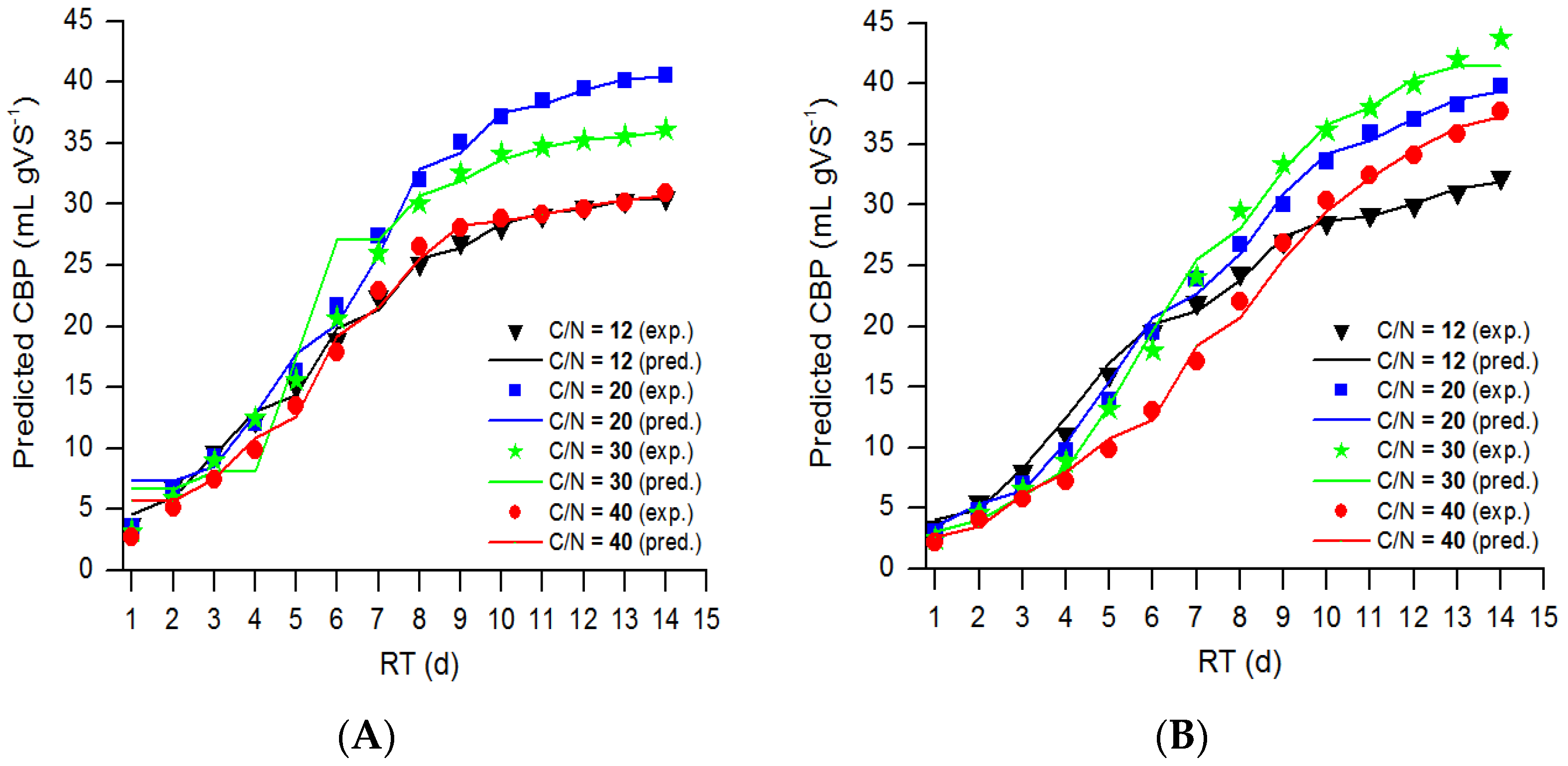
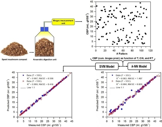
This study aimed to develop, validate, and test two different predictive models based on the AI modeling approach, including k-nearest neighbors and support vector machine (referred to hereafter as k-NN and SVM, respectively) to predict biogas production from anaerobic digestion of spent mushroom compost (SMC). The independent variables involved include temperature, carbon-to-nitrogen ratio (C/N), and retention time (RT). SMC is a bulky residue from mushroom farms, and the waste generated by the mushroom processing industry. It is an ideal source of general nutrients (e.g., nitrogen and phosphorus) and is rich in organic matter that can be used for producing biogas. It is worth mentioning that the nutritional value and the content of organic matter of SMC depend on the types of cultivated mushroom species.
The predictive performance of these models was separately investigated and eventually compared with each other and with the ANN, ANFIS, and logistic models developed by Najafi and Faizollahzadeh Ardabili [31] by means of two statistical indices, including R2, and root mean squared error (RMSE). To the best of the authors’ knowledge, the application of k-NN and SVM modeling approaches to predict biogas production from SMC has never been exploited.

2. Materials and Methods

A schematic portrait depicting the workflow of this study is shown in Figure 2; see text for further details.

2.1. Dataset

The experimental data were taken from the study of Najafi and Faizollahzadeh Ardabili [31]. Briefly, four 2.5 L batch mode anaerobic digesters, each with an effective volume of 1.5 L, were fed with a mixture of SMC and wheat straw (WS) to induce different C/N ratios of 12.2, 20, 30, and 40. The characteristics of SMC and WS are provided in Table 1.
The authors considered the initial TS content of the substrate in the anaerobic digesters as a constant value (8%), and referring to the values of nitrogen and organic carbon for the SMC and WS (Table 1), the contents of SMC and WS in terms of g TS and g VS as a function of C/N ratio were computed as shown in Table 2.
Each anaerobic digester was inoculated with a 10 g bovine rumen solution with a concentration of 1000 g bovine rumen per liter; the bovine rumen solution was kept at a temperature of 37 °C for five days to assist bacteria in growing more rapidly. The anaerobic digesters then were placed in hot water baths at mesophilic temperature (35 °C) and thermophilic temperature (55 °C). The biogas produced from the reactors was measured by a water displacement method for two weeks. All the tests were conducted with three replications. The produced biogas from the reactors was measured by a water displacement method for two weeks. Table 3 shows the experimental data used in this study.

Data Pre-Processing

The dataset shown in Table 3 was used to develop different predictive models compared with those presented by Najafi and Faizollahzadeh Ardabili [31]. As seen in Table 3, the dataset consists of a total number of 112 input–output data pairs (referred to hereafter as observations); the j-th observation contains a collection of 4 data points as { x 1 j , x 2 j , x 3 j , y j } for j = 1 to 112, where x1, x2, and x3 stand for temperature, C/N ratio, and RT, respectively, while y stands for the cumulative biogas production.
Prior to utilizing the dataset to develop a predictive model, it was randomized using Excel (version 2016, Microsoft Corp., Redmond, WA, USA), and then split into two disjoint subsets, including training and testing ones. Ninety observations corresponding to 80% of the dataset were assigned to the training subset, while the remaining 20% of the dataset (i.e., 22 observations) were used as the testing subset. The training subset allowed to adjust the model parameters in order to minimize the error between the experimental data and the model predictions. Meanwhile, the testing subset was employed to evaluate the accuracy of the trained (developed) model for predicting the output. The training and testing subsets were stored in the workspace of MATLAB® (trial version, R2020a) (MathWorks Inc., Natick, MA, USA) in the form of arrays.

2.2. Modeling Approaches

2.2.1. k-NN

The k-NN approach was initially proposed by Fix and Hodges [32] and was later expanded by Cover and Hart [33]. It is recognized as one of the top 10 influential data mining algorithms in machine learning research due to its simplicity in implementation and efficacy in terms of prediction performance [34]. The k-NN algorithm was initially developed with successful application in solving problems with pattern classification, and it was later utilized as a valuable tool for regression purposes. In other words, the k-NN algorithm can be used to predict either class labels or continuous variables. Over the past few decades, k-NN algorithm has attracted impressive attention and is applied in the fields of engineering, science, business, medicine, etc. When using the k-NN algorithm, the main challenges are associated with the determination of the number of neighbors (k), the distance function, and the weighting function [35]. A brief description of the determination of these hyperparameters is provided in the Supplementary Materials (Section A) [36,37,38].
In order to demonstrate how k-NN algorithm is used in developing regression models, let us suppose that Figure 3 shows a number of observations (input–output data pairs) indicated as black square points for a particular system (X stands for the number of observations, and Y stands for its corresponding output). Let the blue square be the query observation whose output is unknown, and suppose that the k-NN algorithm uses five nearest neighbors. The black/red solid lines connecting the query data point with other data points represent the distances, which can be computed based on a distance function specified by the user (e.g., Equation (S1)). The output of the query data point can be estimated by applying a weighting function (e.g., Equation (S4)) considering the distances between the query data point and the five nearest neighbors. The computational procedure of the k-NN algorithm is depicted in Figure 4. It consists of three steps as follows: Step 1 computes the distances between each observation in the testing subset (called query observations) and every observation in the training subset. Step 2 sorts the distances measured from the smallest to the largest, while in Step 3, an appropriate value is assigned to k. Once a weighting function is used, the target output is determined.
Figure 3. A basic illustration of how k-NN algorithm is used in developing regression models. Notes: The solid lines connecting the query data point with other data points represent the distances, which are computed using a distance function specified by the user. The distances from the five nearest neighbors (k assumed to be 5), shown as red solid lines, are considered herein to calculate the output of the query data point using a weighting function specified by the user (see Figure 4 for the detailed computational procedure).
Agriculture 12 01090 g003
Figure 4. A graphical representation of the computational steps of k-NN algorithm for solving regression problems. Notes: The inputs to the algorithm are Xtr, Ytr, Xts, Yts (a column vector with n* elements where all the elements are initially set to zero), and k; Yts is the target output. The reader is referred to Table 4 for the description of the symbols used in this figure.
Agriculture 12 01090 g004
Table 4. Description of the symbols used in Figure 4.
SymbolDescription
XInput matrix, in which each row represents an observation that consists of the values of the input variables
Xts*Repmat (Xts (i,:), n, 1) a
nSize (Xtr,1) b
n*Size (Xts,1) c
mSize (Xtr, 2) d
YA column vector whose i-th element is the output of the i-th observation
DDistance measure (see Equation (S1))
WWeight measure (see Equation (S3))
kNumber of the nearest neighbors (specified by the user)
i, j, r, s, p, and cLoop control variables
D1, lAccumulator variable
a A function found in MATLAB® (trial version, R2020a) (MathWorks Inc., Natick, MA, USA) that produces a matrix consisting of n rows, each is a copy of the i-th row of matrix Xts; b A function that returns the number of rows in matrix Xtr; c A function that returns the number of rows in matrix Xts; d A function that returns the number of columns in matrix Xtr; Subscripts “tr”, and “ts” stand for “training” and “testing”, respectively.
In this study, a k-NN model was developed based on the experimental data (shown in Table 3) using a script written in a MATLAB environment. The Euclidean distance function (Equation (S1)) was used to determine the distances between each query observation (output from the testing subset) and all observations in the training subset. Once all the distances were computed, the k neighbors (k varied from 1 to 10) with the minimum distances from the query observation were assigned a weight (Equations (S2) and (S3)). Thereafter, the output of the query observation was computed in accordance with Equation (S4).
A five-fold cross-validation (CV) approach was performed in order to obtain an optimal value for k. A brief description of an example of a q-fold CV is provided in the Supplementary Materials (Section B) [39].
After determining the optimal k value, the trained model was used to make predictions using the testing dataset, which was unseen throughout the training process.
The k-NN model performance was assessed by two commonly used statistical indices: R2 and RMSE. R2 represents the goodness-of-fit between the measured (actual) values and their corresponding predicted values, which is defined by Equation (1).
R 2 = 1 i = 1 n Y i Y p r e d . , i i = 1 n Y i Y a v g .
RMSE, a measure of the average magnitude of the error, is calculated in accordance with Equation (2):
R M S E = 1 n i = 1 n ( Y i Y p r e d . , i ) 2
where Yi is the actual value of the output, and Ypred.,I is the corresponding model prediction for the i-th observation; Yavg. is the average value of Yi (i = 1, 2, …, n); and n is the total number of observations (in the training or testing subset), on which the R2 and RMSE are estimated.
It is evident from Equations (1) and (2), that the values of R2 closer to one and RMSE closer to zero demonstrate a smaller value of (YiYpred.,I). In other words, the model perfectly fits the data when R2 = 1 and RMSE = 0.

2.2.2. SVM

SVM, a supervised learning technique within the field of computational intelligence, was originally developed at AT&T Bell Laboratories (Holmdel, NJ, USA) by Vapnik [40]. It can be used to solve data classification tasks, which is beyond the scope of this paper and can be extended to solve regression problems, which is the focus of this paper.
Suppose a certain problem is represented by a dataset { ( x i , y i ) } i = 1 n where x i R d is a vector of d input features, y i R is the corresponding scalar output value, and n is the total number of data patterns. The goal of SVM is to find a regression function f ( x ) that estimates the output value whose deviation from the target (actual) value y i , for all x i , is at most epsilon (ε). In other words, an error larger than ε is not tolerated. In addition, f ( x ) should be as flat as possible.
For simplicity, let us first consider the case of a linear SVM regression, which can be expressed in the following form:
f ( x ) = w , x + b
where w R d is the weight vector, b R is the so-called bias term, and w , x denotes the dot product between the weight vector w and vector x that is defined as:
w , x = j = 1 d w j x j
In order to ensure that f ( x ) is as flat as possible, the Euclidean norm of w , i.e., w , should be minimized. This can be represented as a convex optimization problem to minimize:
J ( w ) = 1 2 w 2
subject   to   { i   :   y i w , x i + b ε i   :   w , x i + b y i ε
However, it is necessary to point out that such a function f ( x ) that satisfies these constraints may not exist. Therefore, the slack variables ξ i and ξ i R are required to be introduced. Including the slack variables, Equation (5) can be written as follows (also called the primal objective function):
J ( w ) = 1 2 w 2 + C i = 1 n ( ξ i + ξ i )
subject   to   { i   :   y i w , x i b ε + ξ i i   :   w , x i + b y i ε + ξ i ξ i , ξ i 0 C > 0
where parameter C is a user-defined constant, known as box constraint, which determines the trade-off between the flatness of f ( x ) and the amount up to which deviations greater than ε are acceptable.
To solve Equation (3), it is possible to use the Lagrangian function and optimal constraints, to obtain a linear SVM regression [41] (see Section C in Supplementary Materials for the detailed computational procedure). In the case of a non-linear relationship between the input variables and the output, the SVM model can be simply constructed by mapping the inputs into a high-dimensional feature space, F:
φ   :   R d F
Thus, Equation (S12) can be formulated in the following form (so-called non-linear SVM regression):
f ( x ) = i = 1 n ( α i α i ) K ( x i ,   x ) + b
where the term K ( x i ,   x ) is defined as the kernel function:
K ( x i ,   x ) = φ ( x i ) , φ ( x )
where φ ( x i ) , φ ( x ) is the dot product of the input vectors in the high-dimensional feature space, φ ( x i ) and φ ( x ) .
In order to develop the SVM model, the Regression Learner App in the framework of MATLAB® (trial version, R2020a) (MathWorks Inc., Natick, MA, USA) was used. On the Apps tab, in the Machine Learning and Deep Learning group, the Regression Learner was selected. The training and testing datasets were loaded from the MATLAB workspace, and then a 5-fold CV was chosen as a validation scheme to protect against overfitting.
The key to the establishment of an SVM model is to specify an appropriate kernel function. In addition, the hyperparameters, i.e., kernel scale ( γ ), C, and ε greatly affect the performance of the model, which are typically determined by trial-and-error method. For the system under consideration in this study, four types of kernel functions, including linear, quadratic, cubic, and fine/medium/coarse Gaussian were tested (see Table 5 for the mathematical definition of these kernel functions).
The value of ε was set to 0.001 (the smallest acceptable value in MATLAB R2020a), while the value of parameter C was varied in the range of 0.1 to 10,000 (total number of data points = 23) in order to pick the best model with the least validation error (the smaller the validation error, the better the model generalization ability). Each SVM model was trained with the training subset using the SMO algorithm, considering that the model validation error was estimated by means of a 5-fold CV method (the default validation scheme in MATLAB R2020a). The SMO algorithm stopped iterating when the feasibility gap (see Equation (10)) was less than the pre-specified gap tolerance (the gap tolerance was set to 0.001).
Feasibility   gap   ( Δ ) = J ( w ) + L ( α , α ) J ( w ) + 1
where J ( w ) and L ( α , α ) denote the primal objective (Equation (6)) and the dual objective (Equation (S10)), respectively.
Once the algorithm met the convergence criterion, in other words, the model training process was complete, the trained model was fed as input to make a prediction using the testing dataset. The SVM model performance was assessed by means of the two aforementioned statistical indices (R2 and RMSE; see Equations (1) and (2)).

3. Results and Discussion

3.1. Evaluation of k-NN Model

The optimal k value of the k-NN model was obtained with the aid of a 5-fold CV approach. The optimal k value was defined as the value that allows the k-NN model to produce the smallest RMSE (and the highest R2) on the validation folds in runs 1–5. Figure 5 displays R2 and RMSE values of the validation fold, as a function of the k value varying from 1 to 10, for the k-NN models 1 and 2; k-NN model 1 uses Equation (S2) as the weighting function, whereas k-NN model 2 uses Equation (S3) as the weighting function. It can be seen from Figure 5 that the optimal k value for both k-NN models 1 and 2 was found to be 2; however, model 2 performed better with validation R2 and RMSE of 0.964 and 1.957, respectively, compared with the R2 value of 0.925 and RMSE value 2.969 obtained using model 1. Figure 6 shows the prediction accuracy of k-NN model 2 (k = 2) against the whole dataset under mesophilic condition (35 °C) and thermophilic condition (55 °C) as a scatter plot of the measured and the model-predicted values. As seen in Figure 6, the data points on the plot are well-dispersed around the 45° line (called 100% correlation line or line 1:1) with R2 and RMSE values equal to 0.983 and 1.487, respectively, in the case of mesophilic temperature, and 0.996 and 0.829 in the case of thermophilic temperature, respectively. This implies that only 0.4–1.7% of the total variability in the response cannot be explained by the developed k-NN model 2.

3.2. Evaluation of SVM Model

A 5-fold CV approach was applied to find an appropriate kernel function for the SVM model, and to optimize the parameters C and ε by means of SMO algorithm. Figure 7 illustrates the variation in validation RMSE as a function of the type of kernel function (linear, quadratic, cubic, fine Gaussian, medium Gaussian, and coarse Gaussian), and C value. Parameter C varied from 0.1 to 10,000, whereas ε was set to 0.001. The MATLAB default value was assigned to γ (1.0 for all the linear, quadratic, and cubic functions; 0.43 for the fine Gaussian, 1.73 for the medium Gaussian, and 6.93 for the coarse Gaussian function). As seen in Figure 7, among the different kernel functions that were fitted to the training subset, the coarse Gaussian kernel function yielded the least validation error (RMSE equals 0.932), which was obtained at a C value equal to 1200. The detailed specifications of the trained course Gaussian-based SVM model are tabulated in Table 6.
The prediction accuracy of the coarse Gaussian-based SVM model against the whole dataset under mesophilic condition (35 °C) and thermophilic condition (55 °C) is visualized in Figure 8. This figure indicates an excellent agreement between the measured and the model predicted values with R2 and RMSE values equal to 0.997 and 0.598 in the case of the mesophilic condition, respectively, and 0.999 and 0.418 in the case of the thermophilic condition, respectively. This indicates that only 0.1–0.3% of the total variability in the response cannot be explained by the developed coarse Gaussian-based SVM model.
De Clercq et al. [42] proposed k-NN-, SVM-, and random forest-based models to predict biogas production from “Hainan BioCNG”, an industrial-scale biogas facility located in the south of China, which is capable of treating daily 750 tons of a wide range of agricultural, municipal and industrial bio-wastes, with a daily maximum production of 30,000 m3 bio-methane vehicular fuel. Results indicated that the best performance was achieved by the k-NN model, offering a prediction accuracy of 0.86 and 0.85 on the training dataset and testing dataset, respectively. The SVM and random forest models had accuracy in the range of 0.95–0.97 on the training dataset; however, both of these models produced a testing accuracy far lower (about 0.50) than that of the training accuracy, which shows that the SVM and random forest models were noticeably overfitting the training dataset. The authors claimed that one of the possible reasons for the low testing accuracy of the SVM and random forest models was that the dataset used to tune the hyperparameters was too small. Dong and Chen [43] proposed a novel modeling method, which integrated orthogonal experimental design (OED) with SVM, to establish a relationship between the biogas produced from anaerobic digestion of corn stalk (CS) and the pretreatment process parameters, including mass of CS, ultrasonic duration time, alkali pretreatment time, and single-/dual-frequency ultrasound. The anaerobic digester, composed of a 1.0 L bottle with an effective volume of 0.8 L, operated at pH 7–8, a constant temperature of 35 °C, and at an initial TS and C/N ratio of 15 g/L and 20:1, respectively. The results of the validation experiment demonstrated that OED-SVM was an efficient method for optimizing the pretreatment process parameters and predicting biogas production from anaerobic digestion of CS. In the study performed by Yang et al. [44], two different models, including SVM and ANFIS were developed to estimate biogas production for anaerobic digestion of fruits, vegetables, and food wastes as a function of temperature, pH, VS, biomass type, reactor volume, HRT, organic loading rate, and reactor/feeding type. Findings showed that the proposed SVM model demonstrated a superior capability of predicting biogas with RMSE and R2 of 0.0111 and 0.998 against 0.0683 and 0.946 for ANFIS model. Gao et al. [45] performed a multiple linear regression (MLR) analysis to estimate methane production from anaerobic co-digestion of yellow back fungus spent mushroom and different types of livestock manures (e.g., chicken, dairy, and pig manures) at a constant temperature of 35 °C. The feedstock ratio (spent mushroom-to-manure: 10–90 w/w and TS content (5–15%w)) were considered as the independent variables. From the results, a quadratic polynomial model was found to be a suitable regression model fitting the experimental data, with R2 value greater than 0.95. The author also showed that the Modified Gompertz model could fit the cumulative methane production data with high accuracy (R2 > 0.98). In another study carried out by Kumar et al. [46], two different computational tools, including a feed-forward-backpropagation neural network (FFBPNN) with logistic function, and response surface methodology (RSM) were used to optimize the performance of an electrochemical-assisted anaerobic digester of 1 L capacity fed with the spent mushroom substrate (i.e., wheat straw-based mushroom left over after cultivation of Agaricus bisporus mushroom). Sugar mill wastewater (SMWW), and cow dung were utilized as a supplementary nutrient source and as an inoculum, respectively. The digester temperature (30, 35, and 40 °C), direct electrical current (0, 1.5, and 3 V), and SMWW loading (0, 50, and 100% conc.) were taken as the models’ input variables, whereas the biogas production was the output of the models. The modeling results demonstrated that the FFBPNN models showed an excellent ability to estimate biogas production with a prediction accuracy of 99.91%, which was slightly better than that obtained by the quadratic model of RSM (99.79%). However, from the perspective of error generated, the FFBPNN model produced a smaller RMSE (97.3) compared with that produced by the RSM (117.6).

3.3. Comparison of the Models

Figure 9 illustrates the measured and predicted values for the cumulative biogas production as a function of RT (1 to 14 days) while different levels of temperature (35 °C and 55 °C) and C/N ratios (12, 20, 30, and 40) were investigated. It is evident from Figure 9 that the predicted lines (generated using the developed k-NN and SVM models) follow the trend of experimental data points most closely.
Performance comparison of the k-NN and SVM models is tabulated in Table 7. The results of ANN, ANFIS, and logistic models developed by Najafi and Faizollahzadeh Ardabili [31] are also included in Table 7; two statistical indices (R2 and RMSE between the measured and predicted values) were used in order to make the comparison. It can be observed from Table 7 that the total values of R2 for the developed k-NN model under mesophilic digestion (35 °C) and thermophilic digestion (55 °C) were 0.9830 and 0.9957, respectively. These findings indicate that the k-NN model performs well in predicting biogas production. In addition to its high predictive performance, the k-NN model was straightforward to implement for the problem under consideration because the dataset (composed of 112 observations) and the number of features (i.e., three features) were small. However, it should be noted that in the case of problems that involve several features and a huge dataset, k-NN modeling is not a feasible technique because it is computationally expensive in terms of runtime and memory requirement. Furthermore, the k-NN algorithm calculates and stores the distance of each observation in the testing dataset from all the observations in the training dataset. The total values of R2 for the SVM model under mesophilic digestion (35 °C) and thermophilic digestion (55 °C) were 0.9973 and 0.9989, respectively, which are slightly better than those obtained using the k-NN model (Table 7).
Comparing the performance of the k-NN and SVM models in terms of error produced, the total values of RMSE under mesophilic digestion for the SVM model was 0.5980, which is 58.4% smaller than that obtained using the k-NN model under the same conditions. In the case of thermophilic digestion, the total value of RMSE for the SVM model was 0.4183, which is 49.5% smaller than that obtained using the k-NN model under the same conditions. These results imply that the SVM model is a better choice for predicting biogas production. It is worth mentioning that the SVM modeling technique is less computationally demanding than the k-NN technique and can effectively handle any complex problems involving many features and a massive dataset with high generalization power. However, SVM is very sensitive to the input hyperparameters, and hence, caution must be taken to properly tune the hyperparameters for any given problem. Parameters that may yield an excellent prediction accuracy for problem A may yield a poor prediction accuracy for problem B.
The total values of R2 and RMSE at both mesophilic and thermophilic conditions for the SVM model developed in this study were in the range of 0.9973–0.9989 and 0.4183–0.5980, respectively, which are in agreement with the results of Najafi and Faizollahzadeh Ardabili [31] who developed ANN, ANFIS, and logistic models (R2 = 0.9962–0.9996, RMSE = 0.1940–0.7800). Overall, it can be concluded that the SVM can be a useful alternative tool with the capability of accurately predicting biogas production under both mesophilic and thermophilic conditions.

4. Conclusions

In this study, two data-driven modeling techniques, including k-nearest neighbor (k-NN) and support vector machine (SVM), were successfully trained, validated, and tested to estimate biogas production from anaerobic digestion of spent mushroom compost. It is evident from the results that both the developed k-NN and SVM models can estimate biogas production-under mesophilic and thermophilic conditions-with high prediction accuracy (R2 = 98.3–99.9%). However, the SVM model generated a smaller error (RMSE = 0.418–0.598) than that of the k-NN model (0.829–1.437). These findings imply that the SVM model is a versatile yet more effective tool for predicting biogas production during anaerobic digestion.

Supplementary Materials

The following supporting information can be downloaded at: https://www.mdpi.com/article/10.3390/agriculture12081090/s1, Section A: a brief description of the determination of k-NN hyperparameters; Section B: an example of a q-fold cross-validation (CV) method; Section C: To derive a linear SVM regression with the use of Lagrangian function and optimal constraints; Section D: A solved example of how to use the developed SVM model in this study; Table S1: α values for the support vectors; Figure S1: Schematic illustration of q-fold CV approach; Equations (S1)–(S12).

Author Contributions

Conceptualization, methodology, software, formal analysis, and writing-original draft preparation, R.S.; review and editing, Q.Y. and S.C. All authors have read and agreed to the published version of the manuscript.

Funding

This research was funded by Prince of Songkla University and the Ministry of Higher Education, Science, Research and Innovation, Thailand, under the Reinventing University Project, grant number REV64061 and the APC was funded by the same grant number REV64061.

Institutional Review Board Statement

Not applicable.

Data Availability Statement

Not applicable.

Acknowledgments

The authors thank the support from the Department of Civil and Environmental Engineering, and Research and Development Office, Prince of Songkla University, Thailand. We also thank the support from Biogas and Biorefinery Laboratory at the Faculty of Engineering, and PSU Energy Systems Research Institute, Prince of Songkla University, Thailand.

Conflicts of Interest

The authors declare no conflict of interest.

References

  1. Franta, B. Early oil industry disinformation on global warming. Environ. Polit. 2021, 30, 663–668. [Google Scholar] [CrossRef]
  2. Kaparaju, P.; Rintala, J. Generation of heat and power from biogas for stationary applications: Boilers, gas engines and turbines, combined heat and power (CHP) plants and fuel cells. In The Biogas Handbook: Science, Production and Applications; Wellinger, A., Murphy, J., Baxter, D., Eds.; Woodhead Publishing: Cambridgeshire, UK, 2013; pp. 404–427. [Google Scholar]
  3. Hakawati, R.; Smyth, B.M.; McCullough, G.; De Rosa, F.; Rooney, D. What is the most energy efficient route for biogas utilization: Heat, electricity or transport? Appl. Energy 2017, 206, 1076–1087. [Google Scholar] [CrossRef] [Green Version]
  4. Nasir, I.M.; Mohd Ghazi, T.I.; Omar, R. Production of biogas from solid organic wastes through anaerobic digestion: A review. Appl. Microbiol. Biotechnol. 2012, 95, 321–329. [Google Scholar] [CrossRef] [PubMed]
  5. Caruso, M.C.; Braghieri, A.; Capece, A.; Napolitano, F.; Romano, P.; Galgano, F.; Altieri, G.; Genovese, F. Recent updates on the use of agro-food waste for biogas production. Appl. Sci. 2019, 9, 1217. [Google Scholar] [CrossRef] [Green Version]
  6. Mirmohamadsadeghi, S.; Karimi, K.; Tabatabaei, M.; Aghbashlo, M. Biogas production from food wastes: A review on recent developments and future perspectives. Bioresour. Technol. Rep. 2019, 7, 100202. [Google Scholar] [CrossRef]
  7. Zhang, L.; Loha, K.C.; Zhang, J. Enhanced biogas production from anaerobic digestion of solid organic wastes: Current status and prospects. Bioresour. Technol. Rep. 2019, 5, 280–296. [Google Scholar] [CrossRef]
  8. Uddin, M.M.; Wright, M.M. Anaerobic digestion fundamentals, challenges, and technological advances. Phys. Sci. Rev. 2022. [Google Scholar] [CrossRef]
  9. Tchobanoglous, G.; Burton, F.L.; Stensel, H.D. Wastewater Engineering Treatment and Reuses; McGraw-Hill: New York, NY, USA, 2003. [Google Scholar]
  10. Adekunle, K.F.; Okolie, J.A. A review of biochemical process of anaerobic digestion. Adv. Biosci. Biotechnol. 2015, 6, 205–212. [Google Scholar] [CrossRef] [Green Version]
  11. Sikora, A.; Detman, A.; Chojnacka, A.; Błaszczyk, M.K. Anaerobic digestion: I. A common process ensuring energy flow and the circulation of matter in ecosystems. II. A tool for the production of gaseous biofuels. In Fermentation Processes; Jozala, A.F., Ed.; Intech: Rijeka, Croatia, 2017; pp. 271–301. [Google Scholar] [CrossRef] [Green Version]
  12. Paolini, V.; Petracchini, F.; Segreto, M.; Tomassetti, L.; Naja, N.; Cecinato, A. Environmental impact of biogas: A short review of current knowledge. J. Environ. Sci. Health A 2018, 53, 899–906. [Google Scholar] [CrossRef] [Green Version]
  13. Verbeeck, K.; De Vrieze, J.; Pikaar, I.; Verstraete, W.; Rabaey, K. Assessing the potential for up-cycling recovered resources from anaerobic digestion through microbial protein production. Microb. Biotechnol. 2021, 14, 897–910. [Google Scholar] [CrossRef]
  14. Salehi, R.; Chaiprapat, S. Conversion of biogas from anaerobic digestion to single cell protein and bio-methanol: Mechanism, microorganisms and key factors—A review. Environ. Eng. Res. 2022, 27, 210109. [Google Scholar] [CrossRef]
  15. Hill, D.T. A comprehensive dynamic model for animal waste methanogenesis. Trans. ASAF 1982, 25, 2129–2143. [Google Scholar] [CrossRef]
  16. Mosey, F.E. Mathematical modeling of the anaerobic digestion process: Regulatory mechanisms for the formation of short-chain volatile acids from glucose. Water Sci. Technol. 1983, 15, 209–232. [Google Scholar] [CrossRef]
  17. Pullammanappallil, P.; Owens, J.M.; Svoronos, S.A.; Lyberatos, G.; Chynoweth, D.P. Dynamic model for conventionally mixed anaerobic digestion reactors. AIChE Annu. Meet. 1991, 277C, 43–53. [Google Scholar]
  18. Angelidaki, I.; Ellegaard, L.; Ahring, B.K. A mathematical model for dynamic simulation of anaerobic digestion of complex substrates: Focusing on ammonia inhibition. Biotechnol. Bioeng. 1993, 42, 159–166. [Google Scholar] [CrossRef]
  19. Batstone, D.J.; Keller, J.; Angelidaki, I.; Kalyuzhnyi, S.V.; Pavlostathis, S.G.; Rozzi, A.; Sanders, W.T.M.; Siegrist, H.; Vavilin, V.A. Anaerobic Digestion Model No.1; IWA Publishing: London, UK, 2002. [Google Scholar]
  20. Siegrist, H.; Vogt, D.; Garcia-Heras, J.L.; Gujer, W. Mathematical model for meso- and thermophilic anaerobic sewage sludge digestion. Environ. Sci. Technol. 2002, 36, 1113–1123. [Google Scholar] [CrossRef]
  21. Fedailaine, M.; Moussi, K.; Khitous, M.; Abada, S.; Saber, M.; Tirichine, N. Modeling of the anaerobic digestion of organic waste for biogas production. Procedia Comput. Sci. 2015, 52, 730–737. [Google Scholar] [CrossRef] [Green Version]
  22. Enitan, A.M.; Adeyemo, J.; Swalaha, F.M.; Kumari, S.; Bux, F. Optimization of biogas generation using anaerobic digestion models and computational intelligence approaches. Rev. Chem. Eng. 2017, 33, 309–335. [Google Scholar] [CrossRef]
  23. Cinar, S.; Cinar, S.O.; Wieczorek, N.; Sohoo, I.; Kuchta, K. Integration of artificial intelligence into biogas plant operation. Processes 2021, 9, 85. [Google Scholar] [CrossRef]
  24. Holubar, P.; Zani, L.; Hagar, M.; Froschl, W.; Radak, Z.; Braun, R. Modeling of anaerobic digestion using self-organizing maps and artificial neural nets. Water Sci. Technol. 2000, 41, 149–156. [Google Scholar] [CrossRef]
  25. Cakmakci, M. Adaptive neuro-fuzzy modelling of anaerobic digestion of primary sedimentation sludge. Bioprocess Biosyst. Eng. 2007, 30, 349–357. [Google Scholar] [CrossRef] [PubMed]
  26. Kusiak, A.; Wei, X. Prediction of methane production in wastewater treatment facility: A data-mining approach. Ann. Oper. Res. 2014, 216, 71–81. [Google Scholar] [CrossRef]
  27. Nair, V.V.; Dhar, H.; Kumar, S.; Thalla, A.K.; Mukherjee, S.; Wong, J.W.C. Artificial neural network based modeling to evaluate methane yield from biogas in a laboratory-scale anaerobic bioreactor. Bioresour. Technol. 2016, 217, 90–99. [Google Scholar] [CrossRef] [PubMed]
  28. Dach, J.; Koszela, K.; Boniecki, P.; Zaborowicz, M.; Lewicki, A.; Czekała, W.; Skwarcz, J.; Qiao, W.; Piekarska-Boniecka, H.; Białobrzewskid, I. The use of neural modelling to estimate the methane production from slurry fermentation processes. Renew. Sustain. Energy Rev. 2016, 56, 603–610. [Google Scholar] [CrossRef]
  29. Tan, H.M.; Gouwanda, D.; Poh, P.E. Adaptive neural-fuzzy inference system vs. anaerobic digestion model No.1 for performance prediction of thermophilic anaerobic digestion of palm oil mill effluent. Process Saf. Environ. Prot. 2018, 117, 92–99. [Google Scholar] [CrossRef]
  30. Beltramo, T.; Klocke, M.; Hitzmann, B. Prediction of the biogas production using GA and ACO input features selection method for ANN model. Inf. Process Agric. 2019, 6, 349–356. [Google Scholar] [CrossRef]
  31. Najafi, B.; Faizollahzadeh Ardabili, S. Application of ANFIS, ANN, and logistic methods in estimating biogas production from spent mushroom compost (SMC). Resour. Conserv. Recycl. 2018, 133, 169–178. [Google Scholar] [CrossRef]
  32. Fix, E.; Hodges, J. Discriminatory Analysis—Nonparametric Discrimination: Consistency Properties; USAF School of Aviation: Randolph Field Historic District (near San Antonio), TX, USA, 1951. [Google Scholar]
  33. Cover, T.; Hart, P. Nearest neighbor pattern classification. IEEE Trans. Inf. Theory 1967, 13, 21–27. [Google Scholar] [CrossRef] [Green Version]
  34. Wu, X.; Kumar, V.; Quinlan, J.R.; Ghosh, J.; Yang, Q.; Motoda, H.; McLachlan, G.J.J.; Ng, A.; Liu, B.; Yu, P.S.; et al. Top 10 algorithms in data mining. Knowl. Inf. Syst. 2008, 14, 1–37. [Google Scholar] [CrossRef] [Green Version]
  35. Kang, S. k-nearest neighbor learning with graph neural networks. Mathematics 2021, 9, 830. [Google Scholar] [CrossRef]
  36. Abu Alfeilat, H.A.; Hassanat, A.B.A.; Lasassmeh, O.; Tarawneh, A.S.; Alhasanat, M.B.; Eyal Salman, H.S.; Surya Prasath, V.B.S. Effects of distance measure choice on k-nearest neighbor classifier performance: A review. Big Data 2019, 7, 221–248. [Google Scholar] [CrossRef] [PubMed] [Green Version]
  37. Ehsani, R.; Drabløs, F. Robust distance measures for kNN classification of cancer data. Cancer Inf. 2020, 19, 1176935120965542. [Google Scholar] [CrossRef] [PubMed]
  38. Imandoust, S.B.; Bolandraftar, M. Application of K-nearest neighbor (KNN) approach for predicting economic events: Theoretical background. J. Eng. Res. Appl. 2013, 3, 605–610. [Google Scholar]
  39. Salehi, R.; Lestari, R.A.S. Predicting the performance of a desulfurizing bio-filter using an artificial neural network (ANN) model. Environ. Eng. Res. 2021, 26, 200462. [Google Scholar] [CrossRef]
  40. Vapnik, V.N. The Nature of Statistical Learning Theory; Springer: New York, NY, USA, 1995. [Google Scholar] [CrossRef]
  41. Platt, J.C. Sequential Minimal Optimization: A Fast Algorithm for Training Support Vector Machines; Microsoft Research: Washington, DC, USA, 1998. [Google Scholar]
  42. De Clercq, D.; Jalota, D.; Shang, R.; Ni, K.; Zhang, Z.; Khan, A.; Wen, Z.; Caicedo, L.; Yuan, K. Machine learning powered software for accurate prediction of biogas production: A case study on industrial-scale Chinese production data. J. Clean. Prod. 2019, 218, 390–399. [Google Scholar] [CrossRef]
  43. Dong, C.; Chen, J. Optimization of process parameters for anaerobic fermentation of corn stalk based on least squares support vector machine. Bioresour. Technol. 2019, 271, 174–181. [Google Scholar] [CrossRef]
  44. Yang, Y.; Zheng, S.; Ai, Z.; Molla Jafari, M.M. On the prediction of biogas production from vegetables, fruits, and food wastes by ANFIS- and LSSVM-based models. BioMed Res. Int. 2021, 2021, 9202127. [Google Scholar] [CrossRef]
  45. Gao, X.; Tang, X.; Zhao, K.; Balan, V.; Zhu, Q. Biogas production from anaerobic co-digestion of spent mushroom substrate with different livestock manure. Energies 2021, 14, 570. [Google Scholar] [CrossRef]
  46. Kumar, P.; Kumar, V.; Singh, J.; Kumar, P. Electrokinetic assisted anaerobic digestion of spent mushroom substrate supplemented with sugar mill wastewater for enhanced biogas production. Renew. Energy 2021, 179, 418–426. [Google Scholar] [CrossRef]
Figure 1. A schematic flowchart showing the simple representation of biogas generation during anaerobic digestion process, along with its applications and environmental impacts [10,11,12,13,14]. Notes: a A non-biological process in which the cell walls are physically or chemically broken down to release intracellular substrate. b Biogas release to the atmosphere should be avoided because CO2 and CH4, the main constituents of biogas, are contributors to global warming. c Biogas combustion should be avoided because it is associated with the release of pollutants (e.g., CO, SO2, and NOX) to the atmosphere; SO2, and NOX can react with moisture in the atmosphere to form sulfuric/nitric acid resulting in acid rain. d Solar energy and shale gas, due to being plentiful and cheap, can drive out the biogas application in electricity generation in the near future. e bio-methane can be used as a vehicular fuel or can be injected into the natural gas network. f bio-methanol, and syngas (a mixture of CO and H2) that can be generated via reforming technology. g Biogas can be converted to SCP by the action of methanotrophic bacteria alone, or in combination with autotrophic hydrogen oxidizing bacteria or algae; SCP has excellent potential as an animal feed supplement. Abbreviations: AAs: amino acids; Ac: acetate; Bu: butyrate; LCFAs: long chain fatty acids; MSW: municipal solid waste; Pr: propionate; SCP: single-cell protein; Va: valerate.
Agriculture 12 01090 g001
Figure 2. A schematic illustration of the workflow of this study (a the one that provides the least validation error); see text for further details.
Agriculture 12 01090 g002
Figure 5. Validation curves for (A) k-NN model 1, and (B) k-NN model 2. k-NN models 1 and 2 use Equations (S2) and (S3), respectively, as a weighting function (R2: coefficient of determination; RMSE: root mean squared error).
Agriculture 12 01090 g005
Figure 6. The measured and predicted CBP using k-NN model 2 at 35 °C and 55 °C. R2: coefficient of determination; RMSE: root mean squared error; VS: volatile solids; CBP: cumulative biogas production; k = 2; weighting function: Equation (S3).
Agriculture 12 01090 g006
Figure 7. Validation curve for the SVM model as a function of C and type of kernel function. C: box constraint; R2: coefficient of determination; RMSE: root mean squared error; ε was set to 0.001, which is the smallest acceptable value in MATLAB R2020a.
Agriculture 12 01090 g007
Figure 8. The measured and predicted CBP using the coarse Gaussian-based SVM model. ε = 0.001, C = 1200, and γ = 6.93 under mesophilic condition (35 °C) and thermophilic condition (55 °C); R2: coefficient of determination; RMSE: root mean squared error; VS: volatile solids; CBP: cumulative biogas production.
Agriculture 12 01090 g008
Figure 9. Comparison of measured-predicted CBP using k-NN model 2 at (A) 35 °C and (B) 55 °C and using the best-trained SVM model at (C) 35 °C and (D) 55 °C. CBP: cumulative biogas production.
Agriculture 12 01090 g009aAgriculture 12 01090 g009b
Table 1. Characteristics of SMC and WS [31].
VariableSMCWSUnit
TS19.186.7% g TS/g SMC (or g WS)
VS/TS64.281.7% g VS/g TS
Nitrogen2.40.78% g N/g SMC (or g WS)
Organic carbon2963% g C/g SMC (or g WS)
SMC: spent mushroom compost; WS: wheat straw; TS: total solids; VS: volatile solids.
Table 2. The content of substrate (SMC and WS) fed to the anaerobic digesters as a function of the C/N ratio examined.
C/NSMCWS
Total Mass of SMC (g)TS (g)VS (g)Total Mass of WS (g)TS (g)VS (g)
12.2613.11117.1075.183.212.782.27
20222.9042.5727.3389.3577.4763.29
30105.9520.2412.99115.0599.7581.50
4059.4511.357.29125.26108.6088.73
SMC: spent mushroom compost; WS: wheat straw; TS: total solids; VS: volatile solids; C/N: carbon-to-nitrogen.
Table 3. Biogas production in the experimental-anaerobic digester runs [31].
T = 35 °CT = 55 °C
Exp. CodeC/NRTCBPExp. CodeC/NRT CBPExp. CodeC/NRT CBPExp. CodeC/NRT CBP
E11213.77E33013.20E51213.42E73012.50
26.87 25.87 25.51 24.58
39.69 38.98 37.99 36.56
412.27 412.45 411.10 48.83
515.11 515.59 516.08 513.18
618.92 620.66 619.52 618.02
722.36 725.96 721.95 724.08
825.11 830.07 824.42 829.52
926.88 932.53 927.03 933.37
1028.15 1034.16 1028.56 1036.19
1129.13 1134.74 1129.20 1138.04
1229.78 1235.24 1229.97 1239.99
1330.27 1335.60 1331.04 1342.00
1430.52 1436.11 1432.26 1443.75
E22013.60E44012.75E62013E84012.14
26.64 25.15 24.82 24.06
39.30 37.44 36.98 35.74
412.02 49.88 49.70 47.23
516.35 513.52 513.90 59.87
621.66 617.86 619.54 613.07
727.45 722.91 723.89 717.06
832.06 826.49 826.72 822.07
935.07 928.05 930.01 926.84
1037.15 1028.84 1033.60 1030.41
1138.51 1129.18 1135.99 1132.49
1239.53 1229.58 1237.10 1234.10
1340.15 1330.20 1338.31 1335.90
1440.62 1430.92 1439.83 1437.77
C/N: carbon-to-nitrogen ratio; RT: retention time (d); CBP: cumulative biogas production (mL g VS−1); VS: volatile solids; anaerobic digester’s volume = 2.5 L; operation mode: batch; feedstock: a mixture of spent mushroom and wheat straw.
Table 5. Mathematical definition of the SVM kernel functions and their kernel scales used in this study.
Type of SVM RegressionKernel FunctionKernel Scale (γ)
Linear k ( x , x i ) = γ × x , x i 1
Quadratic k ( x , x i ) = ( γ × x , x i + 1 ) 2 1
Cubic k ( x , x i ) = ( γ × x , x i + 1 ) 3 1
Fine Gaussian k ( x , x i ) = exp ( x x i 2 / ( γ ) 2 ) 0.25 N 0.5
Medium Gaussian N 0.5
Coarse Gaussian 4 N 0.5
x , x i denotes the dot product between the vectors x and xi; x x i denotes the Euclidean distance between the two feature vectors x and xi; the values assigned to γ are the MATLAB default values; N is the number of predictor variables (N = 3 for the system under consideration).
Table 6. Detailed specifications of the best trained SVM model a.
Number of data patterns90
Training algorithmSMO
Convergence criterionFeasibility gap b
Gap calculated9.8398 × 10−4
Gap tolerance1 × 10−3
Number of iterations 27,537
b20.4169
w0.01111
C1200
ε1 × 10⁻³
γ 6.93
nsv90 c
αSee Supplementary Materials (Table S1)
Training runtime d1.175 s
Symbols: b: bias; w: weight; C: box constraint; ε: deviation from the target output value; γ : kernel scale; nsv: number of support vectors, α = α i α i where α i ,   and   α i are the Lagrange multipliers associated with the vector xi whose elements are x1 (temperature), x2 (C/N), and x3 (RT). Abbreviations: SVM: support vector machine; SMO: sequential minimal optimization; C/N: carbon-to-nitrogen; RT: retention time. Notes: a The SVM model constructed based on coarse Gaussian as a kernel function (for a solved example, refer to Section D in the Supplementary Materials). b See Equation (10); the SMO algorithm is converged at an iteration at which the feasibility gap is smaller than the gap tolerance (MATLAB R2020a). c All 90 data patterns are considered as support vectors ( α 0 ); see Supplementary Materials (Table S1) for α values corresponding to the support vectors. d The model was implemented in MATLAB R2020a on a Dell laptop with Intel® Core™ i3-2330M CPU @ 2.20 GHz, and 4.00 GB RAM.
Table 7. Comparison of models developed in this study and those developed by Najafi and Faizollahzadeh Ardabili [31].
T (°C)C/N Models Developed in This StudyModels Developed by Najafi and Faizollahzadeh Ardabili [31]
k-NNSVMANNANFISLogistic
R2RMSER2RMSER2RMSER2RMSER2RMSE
35120.99580.58990.99950.198610.03640.99940.23460.99860.4094
200.99031.30760.99670.75840.99421.30640.99980.22020.9990.5
300.95922.37860.99810.51660.99660.77560.99980.14750.99840.5327
400.98881.06480.99460.74080.99920.36060.99980.15930.99740.5865
Total0.9831.43740.99730.5980.99620.780.99960.1940.99840.5111
55120.99610.60680.99810.4220.99840.55840.99920.2860.99720.5691
200.99610.80850.99780.60230.99980.20040.9990.42330.99840.5501
300.99511.01850.99940.35540.99980.27330.99980.25120.99860.5771
400.99560.83040.99980.18110.99980.20930.99980.20980.99860.5035
Total0.99570.8290.99890.41830.99840.3430.99940.30330.99820.5506
k-NN: k-nearest neighbors; SVM: support vector machine; ANN: artificial neural network; ANFIS: adaptive neuro-fuzzy inference system; R2: coefficient of determination; RMSE: root mean squared error; C/N: carbon-to-nitrogen.
Publisher’s Note: MDPI stays neutral with regard to jurisdictional claims in published maps and institutional affiliations.

