Simulating Spring Barley Yield under Moderate Input Management System in Poland

Abstract

In recent years, forecasting has become particularly important as all areas of economic life are subject to very dynamic changes. In the case of agriculture, forecasting is an essential element of effective and efficient farm management. Factors affecting crop yields, such as soil, weather, and farm management, are complex and investigations into the relation between these variables are crucial for agricultural studies and decision-making related to crop monitoring, with special emphasis for climate change. Because of this, the aim of this study was to create a spring barley yield prediction model, as a part of the Advisory Support platform in the form of application for Polish agriculture under a moderate input management system. As a representative sample, 20 barley varieties, evaluated under 13 environments representative for Polish conditions, were used. To create yield potential model data for the genotype (G), environment (E), and management (M) were collected over 3 years. The model developed using Multiple Linear Regression (MLR) simulated barley yields with high goodness of fit to the measured data across three years of evaluation. On average, the precision of the cultivar yielding forecast (expressed as a percentage), based on the independent traits, was 78.60% (Model F-statistic: 102.55***) and the range, depending of the variety, was 89.10% (Model F-statistic: 19.26***)–74.60% (Model F-statistic: 6.88***). The model developed using Multiple Linear Regression (MLR) simulated barley yields with high goodness of fit to the measured data across three years of evaluation. It was possible to observe a large differentiation for the response to agroclimatic or soil factors. Under Polish conditions, ten traits have a similar effect (in the prediction model, they have the same sign: + or -) on the yield of almost all varieties (from 17 to 20). Traits that negatively affected final yield were: lodging tendency for 18 varieties (18-), sum of rainfall in January for 19 varieties (19-), and April for 17 varieties (17-). However, the sum of rainfall in February positively affected the final yield for 20 varieties (20+). Average monthly ground temperature in March positively affected final yield for 17 varieties (17+). The average air temperature in March negatively affected final yield for 18 varieties (18-) and for 17 varieties in June (17-). In total, the level of N + P + K fertilization negatively affected the final yield for 15 varieties (15-), but N sum fertilization significantly positively affected final yield for 15 varieties (15+). Soil complex positively influenced the final yield of this crop. In the group of diseases, resistance to powdery mildew and rhynchosporium significantly decreased the final yield. For Polish conditions, it is a complex model for prediction of variety in the yield, including its genetic potential.

1. Introduction

Barley (Hordeum vulgare L.) is grown in almost all parts of the world for human consumption, industry, and animal feed. It ranks fourth in the world, after wheat, maize, and rice, in terms of growing area. Almost half of the world’s barley growing area is located in Europe, where it ranks second after wheat in terms of growing area. Barley can grow in unfavorable agroclimatic conditions because of its ability to tolerate late sowing and moderate levels of drought stress, which are very important in a changing climate [1,2,3]. Comparative studies on wheat and barley [4,5] suggest that the higher yielding ability of barley in drier environments is largely due to earlier commencement of flowering and maturity and a faster rate of leaf canopy development and root growth early in the season, when vapor pressure deficit is low. Their study explained that barley and wheat characteristics result in reduced evaporative loss of water from the soil surface and increase water use efficiency (WUE) for above-ground biomass production, which makes barley a good candidate to replace wheat under severe climate change conditions.

Efforts to identify suitable barley varieties, as well as other crops, with yield-enhancing characteristics in various climatic conditions, considering climate change, remain essential to developing sustainable agriculture and food security [6,7,8,9,10]. Yield is complex and governed by several genes that interact with the environment. Consequently, the selection of genotypes based on performance in a single environment is ineffective [11]. Thanks to the forecasts applied by the use of appropriate test methods, in marginal environments, the risk of error can be greatly reduced.

In recent years, forecasting in agricultural production has become particularly important, as all areas of agriculture are subject to very dynamic changes. Forecasting based on proper models is an essential element of effective and efficient farm management [12,13]. An accurate and timely forecast of yields during the vegetation season is the basis for estimating production volumes during the harvest. Moreover, early information on the future allows farmers to plan and organize their purchases, storage, and processing of agricultural crops [8,9,11,13,14,15,16,17,18,19,20,21,22,23,24,25,26,27,28].

Many factors influence the quantity and quality of yields. Because of this, different author have used other parameters to predict them during the growing season, which may be proper where they carried their studies. One of the most important factors affecting plant development is weather, which it is why the constructed models should take into account meteorological data (e.g., air temperature, rainfall, insolation) [8,15,24,29,30,31,32]. Moreover, the second group of traits influencing plant development is connected with the soil and they should be taken into account in the models under construction: pH, structure, organic material content, and nutrient levels [11,23,25,33,34,35,36]. Proper management, including fertilization, harvesting technology, and tillage technologies, of crop rotation has a positive effect on soil structure and the availability of water for plants. The soil– water system remains the crucial element of the ecological framework, on which food production and water resource management depend directly, which is so important in terms of a changing climate.

The average global temperature is rising due to the increasing release of greenhouse gases (GHGs) into the atmosphere. This change in climate can reduce agricultural yields, resulting in food insecurity. However, agricultural activities are one of the major contributors of GHGs and lower yields can trigger increased activity to meet the demand for food, resulting in higher quantities of GHGs released into the atmosphere [8,20,37,38]. Global warming can reduce the net carbon gain by increasing plant respiration rates, which decrease the production yield of crops and could even result in the invasion of weeds, pathogens, and pests.

Pest challenges vary over seasons and it is difficult to predict how this variation will shift in the face of climate change and may render resistant plants to susceptible ones [39,40,41,42,43,44]. This is why the constructed models for forecast of yields and its quality during the vegetation season should take these changes into account [9,39,40,43,45]. This capability is essential to create new varieties resistant to changed pest pressure. Plant–pest interactions, such as changes in plant resistance and plant phenology, have an impact on co-occurrence, with more generations of pests per year, more virulent new pathotypes in the population, and differences in plant primary and secondary metabolism under elevated carbon dioxide levels. Disease management programs or climatic extremes keep pathogen population size small, limit gene diversity, and help to control the disease. The widespread prevalence of barley cultivation in Europe, the use of both spring and winter forms, and local climatic conditions promote the persistence of the pathogen and the development of the disease of this crop [46,47]. For barley, depending on the environment, the most important foliar fungal pathogens may be powdery mildew, net blotch, scald, spot blotch, barley stripe, and leaf rust [48,49,50,51,52]. They can cause a 10–40% yield loss depending on barley growing areas. Powdery mildew is caused by Blumeria graminis f. sp. hordei and may have the greatest negative impact on yield [53,54,55,56,57,58]. Net blotch in barley is caused by Pyrenophora teres f. teres (anamorph: Drechslera teres) and this pathogen has two forms: P. teres f. maculata causes the spot form and P. teres f. teres causes the net form of the disease. These diseases reduce the green leaf area and grain size and have a big impact on the malt quality [44,59]. Rhynchosporium commune causes scald disease in barley. This disease is more common in cooler and semi-humid regions [44,60,61,62,63]. Cochliobolus sativus (anamorph: Bipolaris sorokiniana) is the causal agent of spot blotch disease. Barley stripe disease is caused by the fungal pathogen Pyrenophora graminea (anamorph: Drechslera graminea). It is present in many regions of the world, including Europe, China, Russia, India, North Africa, Turkey, and North America [59,60,61,62,63,64]. This disease manifests itself as chlorotic and necrotic areas in the leaves and heads and also significantly affects the yield. Over the last few years, the most important is barley leaf rust pathogen Puccinia hordei, which forms spherical light-orange-brown pustules on leaves. In many regions around the world, in susceptible varieties during an epidemic, this is lowering the yield by up to 62% [65,66,67,68,69]. In Central Europe, leaf rust ranks second after powdery mildew among the most common diseases in barley [70,71].

A large number of approaches, such as crop models, algorithms, and statistical tools, have been proposed and used for yield prediction in precision agriculture. These methods are used to minimize the problem caused by interacting variables to facilitate the interpretation of complex relationships to reduce the dimensionality in the data set or select a subset of appropriate variables from a large data set [72,73,74]. Subsequent attempts have been made by applying artificial intelligence principles and soft computing techniques in precision agriculture for spatial analysis and crop management [13,37,38,75].

As described by [73], nonlinear models, such as APSIM [76], DSSAT [77], RZWQM, and SWAP/WOFOST [78], combine many traits, such as physiological and phenotypic variation at different phases of the growth cycle measurement data. Because this calibration of model coefficients can be labor intensive and time consuming [26,27,28,29,79,80], computation speed could be low and prediction accuracy may not be as high as some machine learning algorithms. Model ANNs (artificial neural networks), as no-linear statistical techniques, have been applied to investigate yield response to soil variables [16,75,81]. Specifically, ANN analysis as applied in precision agriculture for spatial analysis and crop management [16,33,82] The observed data set for the selected variables is fitted to describe the problem by adjusting the weights of linkages connecting input and output variables and can be regarded as multivariate non-linear analytical tools. Further, as described by the authors, its limitation is the need for a large amount of data for training.

In agriculture, principal component analysis (PCA) and factor analysis (FA), with multiple regressions, are the methods that were applied for the construction models to predict yield and identify important factors influencing yield [16,73,83,84,85]. In the case of MLR analysis, the description of linear relationships between crop parameters and site variables is limited and the results may be misleading when these relationships are not linear. Thanks to this, it is possible not only to create a prediction and simulation model, but also to make a weight evaluation of all independent variables included in the model [16,17,24,33,73,84,85,86,87,88,89].

Because of this, the aim of this study was to create a barley yield prediction model as a part of the Advisory Support platform in the form of application for Polish agriculture under a moderate input management system. Multiple Linear Regression (MLR), based on the environmental (E), genetic (such as variety in disease resistance and yield potential) (G), and management (M) traits in multi-environmental conditions, was used.

2. Materials and Methods

2.1. Plant Material

As a plant material 20 varieties were used (Soldo, Radek, RGT Planet, KWS Olof, Basic, Ella, KES Astrika, Oberek, KWS Irina, Salome, Rubaszek, Podarek, Alianz, KWS Cantton, KWS Harris, KWS Vermont, Paustian, Polonia Staropolska, Ringo).

2.2. Experimental Design, Management System, and Growing Conditions

The data used in this study to build forecast models comprise 13 experimental sites of the Research Centre of Cultivar Testing (COBORU) in Poland observed in the Post Registration Variety Testing System (PVTS) where the yield and other related traits of newly released varieties were evaluated in multi-environmental trials during the three cropping seasons 2016, 2017, and 2018 (

Table 1. List of locations of post-registration multi-environment variety system testing trials (PRVTS) conducted in moderate input management system, their symbol code, part of Poland symbol codes, and information about geographic localization.

Part of Poland	Part of Poland Code	Location	Location Code	Latitude (φ)	Longitude (λ)	Altitude (m)
North-West	NW	Białogard	L1	54°00′	15°59′	32.0
North	N	Radostowo	L2	53°98′	18°75′	40.0
North-East	NE	Ruska Wies	L3	53°47′	22°12′	15.8
North-East	NE	Krzyzewo	L4	53°01′	22°46′	135.0
Central	NE	Nowa Wies Ujska	L5	53°03′	16°75′	105.0
Central	C	Glebokie	L6	52°65′	18°43′	85.0
Central	C	Sulejow	L7	51°21′	19°52′	188.0
Central	C	Kaweczyn	L8	52°10′	20°21′	90.0
South	S	Glubczyce	L9	50°18′	17°83′	280.0
South	S	Pawlowice	L10	49°57′
Central-Weast	C	Slupia	L11	50°63′	19°96′	290.0
East	E	Cibór Duży	L12	52°08′	23°11′	114.0
South-East	SE	Przecław	L13	49°53′	22°44′	230.0

).

Locations were scattered across different agroclimatic regions of Poland, because this country represents transitional zone between sea and continental climate transition: S—south; N—north; W—west; SE—southeast; and NE—northeast. Geographical locations of the experimental fields were as follows: latitude ranging from 50.1928° N to 52.9818° N, longitude from 15.0776° E to 21.445° E, and altitude from 77 to196 m above sea level (Table 1).

Each trial was established as a randomized block design with three blocks and plots of 10 m² (10 seed rows 8 m long and 1.3 m wide). The trials were planted depending on the year and part of Poland between 15.03 and 5.04. They were conducted as moderate input intensity experiments with mineral fertilization including nitrogen, phosphorus, and potassium adapted to the conditions in each location (

Table 2. Management of the trials across the thirteen environments and three years: mineral fertilization including nitrogen, phosphorus, and potassium adapted to the conditions in each location (soil types).

Management of the Trials Across the Thirteen Environments and Three Years
No.	Location	Soil Complexity	2016					2017					2018
			N	Sum of N	P2O5	K2O	Sum of NPK	N	Sum of N	P2O5	K2O	Sum of NPK	N	Sum of N	P2O5	K2O	Sum of NPK
1	Białogard	4	300	120	60	120	300	300	110	60	120	290	300	120	60	120	300
2	Radostowo	1	300	94	42	112	248	300	80	60	102	242	300	88	70	105	263
3	Ruska Wieś	2	300	70	60	70	200	300	70	40	90	200	300	70	60	90	220
4	Krzyżewo	4	300	50	60	90	200	300	60	60	90	210	300	88	36	102	226
5	Nowa Wieś Ujska	4	300	90	70	105	265	300	90	48	80	218	300	108	24	24	156
6	Głębokie	2	300	70	30	80	180	300	72	24	70	166	300	72	24	68	164
7	Sulejów	2	300	91	25	70	186	300	96	30	70	196	300	120	40	70	230
8	Kawęczyn	4	300	62	45	90	197	300	95	45	90	230	300	80	45	90	215
9	Cicibór	4	300	63	40	60	163	300	92	40	60	192	300	89	40	60	189
10	Głubczyce	1	300	40	60	90	190	350	36	0	0	36	300	81	47	40.7	169
11	Pawłowice	3	300	128	84	84	296	300	90	36	75	201	300	90	72	72	234
12	Słupia	2	300	113	50	70	233	300	117	59	70	246	300	107	50	70	227
13	Przecław	2	300	60	40	60	160	300	80	60	90	230	300	103	70	105	278

). The lowest N applied was 40 kg N × ha⁻¹ and the highest was 120 kg N × ha⁻¹ in 2016. In 2017 the range for N sum was 36–117 kg N × ha⁻¹ and in 2018: 72–120 kg N × ha⁻¹. P₂O₅, K2) and NPK (Supplementary 1).

The harvest area of each plot was 10 m². Spring barley was planted at end of March and beginning of April. It was harvested at the end of July.

2.3. Collected Data Set

Multiple regression was preceded by examination of the determination coefficient R2 for the examined variables. It was carried out based on the impact of environmental data (weather: precipitation, daily air temperature, and soil temperature), the degree of resistance to biotic stresses (fungus), as well as on the average yield from the last 3 years, the amount of fertilization applied, and the soil complex.

• List of quantitative and qualitative data:

  ―

  Constant—the constant obtained during the analysis (called regression constant),

  ―

  Yield as the amount of seeds as tons of seed dry matter per hectare (dt ha⁻¹) across 3 years (2016–2018) and across all locations (as a genetic potential of the genotype),

  ―

  NPK sum—NPK fertilization, sum,

  ―

  N sum—nitrogen mineral fertilization N -sum,

  ―

  Compl—soil complex valuation classes according to the soil quality evaluation system in Poland compatible with regulations of the Council of Ministers; class reflects the agricultural value of soils and a lower class means more fertile soils; (converted into a synthetic indicator according IUNG-PIB Pulawy),

  ―

  LT-lodgbfhar—lodging tendency before harvesting,

  ―

  Disease resistance: PM (powdery mildew), NB—net blotch, BBR (barley brown rust), SB (rhynchosporium); disease resistance was scored on 1–9 scale (9—no symptoms of the disease).

• Weather environmental variables

  ―

  The sum of rainfall: o1—in January, o2—in February, o3—in March, o4—in April, o5—in May, o6—in June, and o7—in July,

  ―

  Average monthly ground temperature: tg1—in January, tg2—in February, tg3—in March, tg4—in April, tg5—in May, tg6—in June, and tg7—in July,

  ―

  Average daily air temperature: tp1—in January, tp2—in February, tp3—in March, tp4—in April, tp5—in May, tp6—in June, tp7—in July.

2.4. Calculation Methodology

Statistical modelling of the causal relationship between yield and agrotechnical and weather factors was carried out using a multiple regression model [90,91,92]. The variables for the model were selected using the backward selection method. The model with the best fit (highest adjusted determination factor) to the observed data was wanted. Model parameter values, standardized parameter values, and determination coefficients were estimated. Analyses were carried out separately for each variety and then for the whole group of the evaluated barley varieties (the model with the highest adjusted coefficient of determination). Calculations were made in GenStat 21 (VSN International, England, UK, 2020) and Statistica 13.3 (TIBCO Software Inc., Palo Alto, CA, USA, 2017) software [93,94].

3. Results

3.1. Identification of Weather Environmental Variables Used in Multivariate Regression Analysis

Significant differences between locations and years for precipitation and temperatures were observed (

Table 3. Monthly average daily air temperature, ground temperature, and sum of rainfall across the thirteen environments where experiments with barley were conducted (2016–2018).

Supplementary Monthly Average Daily Air Temperature, Ground Temperature and Sum of Rainfall
Average Daily Air Temperature												Average Monthly Ground Temperature												the Sum of Rainfall
2016				2017				2018				2016				2017				2018				2016				2017				2018
Month	Average	Min.	Max.	Month	Average	Min.	Max.	Month	Average	Min.	Max.	Month	Average	Min.	Max.	Month	Average	Min.	Max.	Month	Average	Min.	Max.	Month	Average	Min.	Max.	Month	Average	Min.	Max.	Month	Average	Min.	Max.
I	−3.2	−5.7	−1.9	I	−4.2	−6.2	−1.0	I	0.7	−1.4	2.7	I	−1.5	−3.1	0.6	I	−1.2	−2.3	0.8	I	0.4	−0.4	1.4	I	28.3	11.3	45.1	I	18.3	10.7	42.1	I	32.6	18.3	65.6
II	3.2	1.5	4.0	II	−0.7	−2.3	0.6	II	−3.3	−5.1	−2.2	II	1.9	1.0	2.8	II	−0.8	−2.1	0.4	II	−1.3	−2.1	−0.1	II	60.9	23.5	91.9	II	33.5	17.7	55.5	II	11.8	4.9	24.7
III	3.8	2.7	4.7	III	5.7	4.3	6.3	III	0.1	−1.5	1.3	III	2.6	1.9	4.4	III	3.3	2.7	5.7	III	−0.5	−1.3	1.1	III	31.3	13.9	69.7	III	44.4	19.5	70.8	III	28.0	18.0	53.1
IV	8.5	7.9	9.8	IV	7.1	6.0	7.7	IV	12.5	11.0	13.4	IV	7.0	5.6	10.4	IV	5.8	5.0	8.7	IV	9.0	7.3	13.1	IV	32.5	12.8	57.0	IV	74.4	34.8	145.3	IV	29.4	9.4	61.4
V	14.4	13.3	15.6	V	13.3	12.4	14.1	V	16.2	14.5	17.4	V	13.7	12.0	18.0	V	12.6	10.7	16.8	V	15.3	13.1	17.6	V	45.2	12.2	108.3	V	51.9	19.6	111.9	V	41.9	9.4	68.8
VI	17.9	17.0	18.6	VI	17.3	16.4	18.7	VI	18.0	16.8	18.7	VI	18.2	16.0	22.2	VI	17.4	15.1	21.1	VI	18.6	16.5	20.4	VI	71.0	23.8	168.9	VI	76.8	26.3	174.4	VI	46.2	22.5	93.3
VII	19.1	18.0	19.9	VII	18.1	16.7	19.2	VII	20.0	18.1	21.0	VII	18.7	16.6	21.6	VII	18.0	16.0	21.0	VII	19.2	17.7	20.5	VII	154.5	86.0	408.2	VII	91.0	44.4	166.1	VII	106.4	80.7	131.2

). The 2017 growing season was the coldest year, with high rainfall, and 2018 was hot and dry. Average air temperatures in 2018 in April were higher in all locations by more than 3.0 °C compared to averages in 2016 and 2017, while, on average, by 1.0 in the remaining months.

Depending on the location, the maximum air temperatures in 2018 were higher compared to 2017 for the entire growing period (from 3.6 to 7.8 °C in April, from 2.1 to 3.9 in May, from 0.1 to 4.3 in June and from 1.4 to 6.3 °C in July). In 2017, maximum temperatures in April reached 17.8 °C, May 23.8 °C, in June 27.0 °C, and in July 26.2 °C. In 2016, the maximum temperature in May was 26.0 °C. During the 2018 growing season, the maximum temperature in April was 23.6 °C, in May 26.1 °C, in June 27.6 °C, and in July 30.2 °C.

In January 2016 and 2017, average air temperatures were in a range from −6.2 °C to −1.0 °C and in 2018, in a range from −1.4 °C to 2.7 °C. In February, the highest temperatures were in 2016 (average +3.2 °C, range −1.5 °C–4.0 °C), they were, on average, in 2017, −0.7°C (range from −2.3°C to 2.5°C), and in 2018, on average, were −3.3°C (range from −5.1 °C to −2.2 °C). In March, average air temperatures in 2017 were in a range from 4.3 °C to 6.3 °C (average 5.7 °C) and in 2018, in a range −1.5 °C–1.3 °C (on average −0.1 °C). In April and May 2018, the average air temperatures were, on average, 4.0 °C higher than in 2017 and 2016.

In January and February, similar to the average temperatures, ground temperatures were lowest in 2018. In March 2018, they were also below zero (in a range −1.7–1.8), which is about 3–4 degrees higher than in 2017–2018. On average, the temperatures for all years were similar, and only in 2016, in June, the maximum temperatures were higher than in other years. On average, throughout the growing season, the amount of rainfall was lower compared to 2016 and 2017.

Drought occurred in many locations. The differences were approx. 10 mm compared to 2016 and approx. 20 mm compared to 2017. The differences between the locations were large over the years.

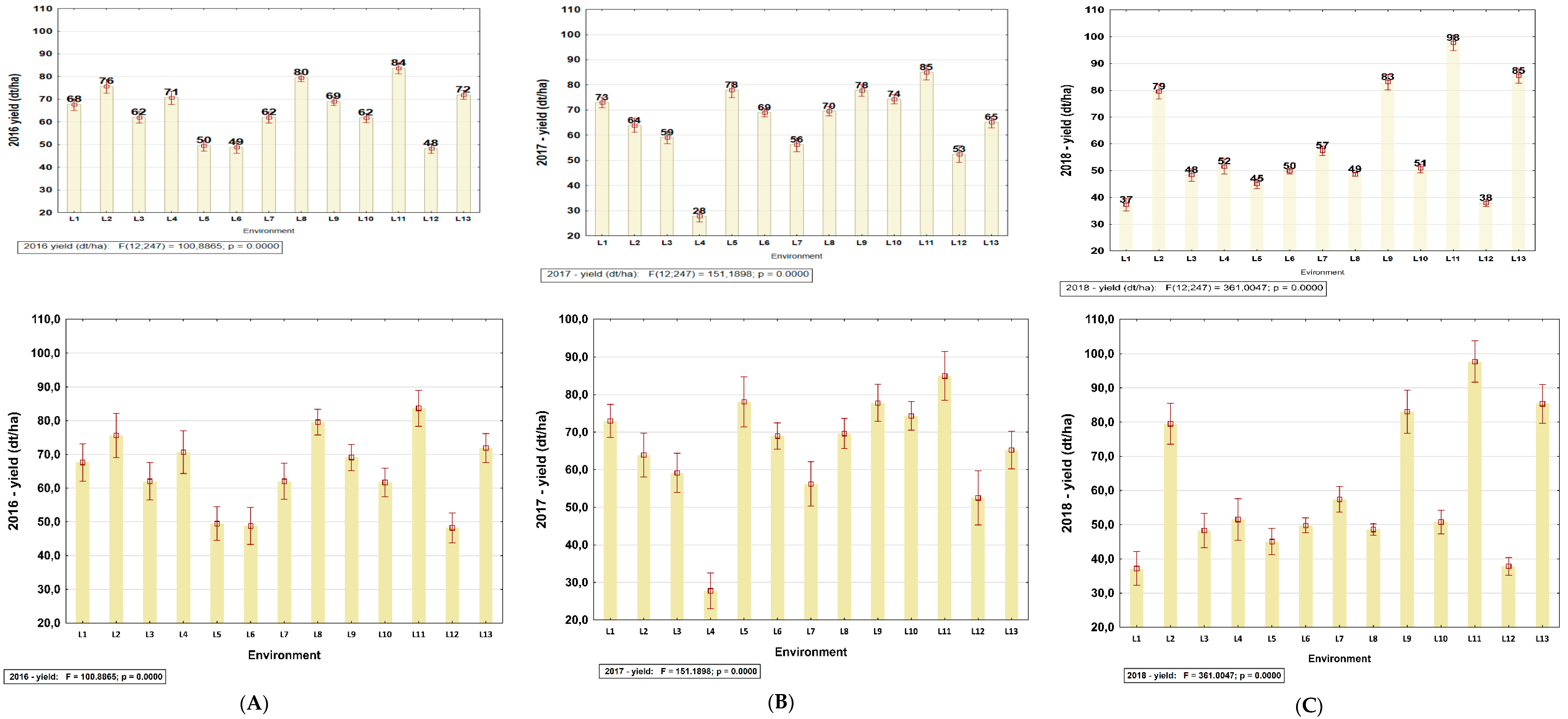
3.2. Identification of Yield Information for Site–Years Used in this Study

The variation in spring barley grain yield in the analyzed period (2016–2018) was relatively high and differences between years and locations were significant (Figure 1 and Figure 2, Supplementary 1). On average, in 2016 and 2017, the yield was similar, and in 2018, it was very low. Across all years, the highest yields were in L11 (Slupia).

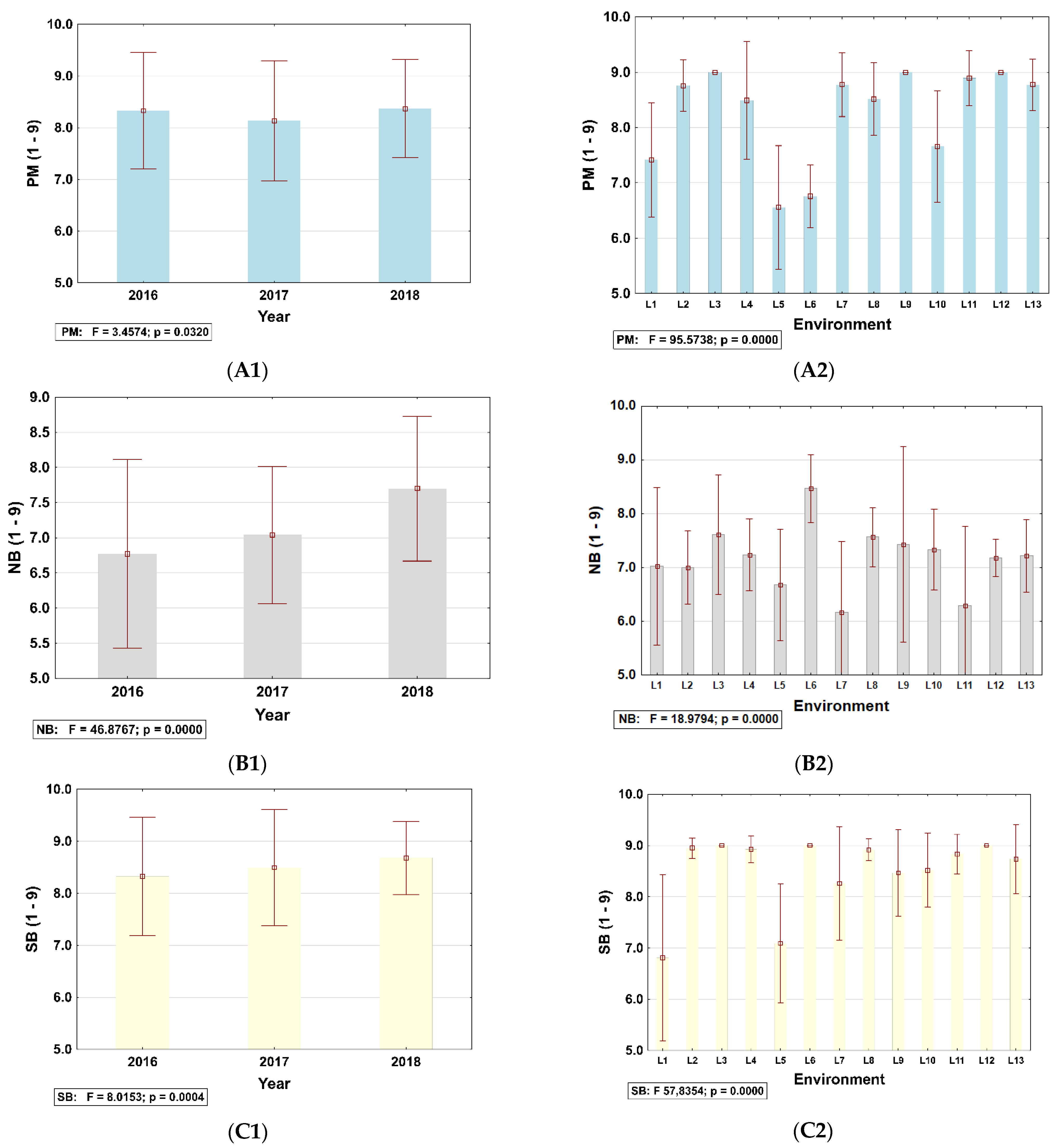
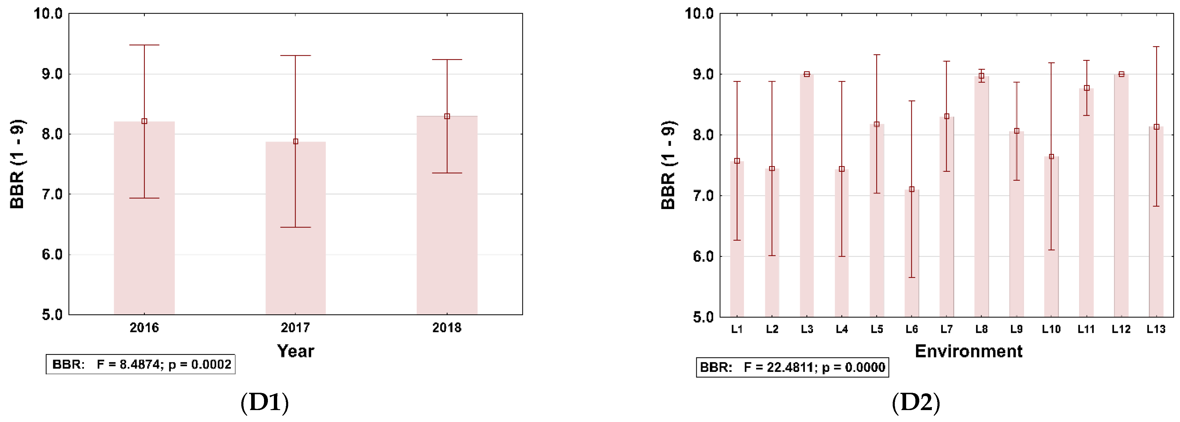
3.3. Identification of Disease Information for Site–Years Used in This Study

The variation in spring barley resistance for the most economically important diseases, such as powdery mildew (PM), net blotch (NB), and barley brown rust (BBR) in the analyzed period (2016–2018) was relatively high and differences between years and locations were significant (p < 0.05, Figure 3A1–D1, Supplementary 1).

Differences for PM severity across years were not significant (8.1–8.4 in 1–9 scale, where 1 means no symptoms of the disease); however, they were significant between the locations, in a range from 6.6 (L5) to 9.0 (L3, L12) (p < 0.05, Figure 3A2). On average, significant differences between years were observed for NB disease (in a range from 6.8 in 2016 to 7.7 in 2018, p < 0.05) (Figure 3B1). In locations L5 and L7, NB severity was high and scored 6.7 and 6.2, respectively (Figure 3B2). Differences for BBR (BBR) were significant between years (p < 0.05, Figure 3D1) and between localities (p < 0.05, Figure 3D2).

3.4. Impact of Diseases on Yield Potential

Phenotypic data for PM, SR, and BBR severity at MW stages in 2016, 2017, and 2018 are presented in the Supplementary File 1. Summary statistics are presented on the Figure 3A1,A2 for PM, Figure 3B1,B2 for NB, Figure 3C1, C2 for SB, Figure 3D1, D2 for BBR. Frequency distribution models for the spring barley varieties based on PM, NB, NS, and BBR and with the regression analysis models to estimate the relationship between resistance scores and frequency index are presented in Figure 4.

3.5. Regression Models

The final yield AGRO-SBY prediction model of 20 varieties, grown in the 13 locations, was conditioned by its genetic potential, including disease resistance, which was modified by environmental conditions. In the location where data were collected, there was a large intra-species differentiation for the response to agroclimatic or soil factors (soil structure, availability of micro and macro elements) and this is presented in Table 1 and Table 2. It was possible to observe significant differentiation between the evaluated varieties for yield potential, disease resistance, and lodging tendency, and this is presented in Supplementary 1.

Comparison between yield harvested and predicted based on AGRO-SBY model of 20 varieties in thirteen environments (L1–L13) in 2016, 2017, and 2018 is presented in Supplementary 3. Comparison between yield predicted and harvested in 2016, 2017, and 2018 based on the average in thirteen environments is presented in Figure 5.

Estimated model parameter values, standardized parameter values, and determination coefficients were estimated for each of the 20 varieties (

Table 4. R-squared AGRO-SBY yield prediction models developed using MLR method for twenty varieties based on the data collected in thirteen locations including genetic potential, environment, and management traits under moderate input management system.

No.	Variety	Model F-Statistic	R sq. adj.	No.	Variety	Model F-Statistic	R sq. adj.
1	Soldo	6.88 ***	0.746	11	Salome	6.93 ***	0.766
2	Radek	10.34 ***	0.831	12	Rubaszek	8.73 ***	0.785
3	RGT Planet	12.82 ***	0.848	13	Podarek	10.33 ***	0.797
4	KWS Olof	11.52 ***	0.816	14	Allianz	8.62 ***	0.822
5	Basic	8.53 ***	0.79	15	KWS Cantton	12.22 ***	0.842
6	Ella	7.72 ***	0.75	16	KWS Harris	9.19 ***	0.812
7	KWS Atrika	8.05 ***	0.796	17	KWS Vermont	19.26 ***	0.891
8	Oberek	9.47 ***	0.791	18	Paustian	10.28 ***	0.843
9	KWS Iri	8.22 ***	0.774	19	Polonia Staropolska	7.93 ***	0.745
10	KWS Dante	6.12 ***	0.719	20	Ringo	7.26 ***	0.776

***—significant at α = 0.01.

, Supplementary 2). The R-squared, which measures the strength of the relationship between the AGRO-SPY model and the dependent variable for each variety, was relatively very height (range: 74.6% for Soldo–89.1% for KWS Vermont).

Based on the models for 20 varieties, it was possible to observe that among the independent (explanatory) traits included in the analysis, the following types can be distinguished as two groups (Supplementary 2):

(1)

Ten traits have a similar effect (in the prediction model they have the same sign) on the yield of almost all varieties (i.e., u from 17 to 20). This is, e.g., a lodging tendency (LT) that occurred in the prediction model for 18 cultivars with a plus sign, and we write: (18-). Other traits are: o1 (19-), o2 (20+), tg3 (17+), tg4 (17-), tp3 (18-) and tp6 (17).

(2)

Twenty traits have a similar effect on the yield of more than half of the studied cultivars: o4 (16-), o7 (16-), tp2 (15+), tp4 (13+), tp7 (14+).

In total, the level of N + P + K fertilization negatively influenced the final yield (15-). However, Nsum fertilization was significantly positive (15+). In the group of diseases, resistance to powdery mildew and rhynchosporium significantly decreased the final yield, while the other diseases did not. Other traits influenced the yield of less than half of the studied cultivars (in the same or differently).

The model for the whole group of the 20 evaluated barley varieties (the model with the highest adjusted coefficient of determination) is presented in

Table 5. Regression model for spring barley yield prediction (AGRO_SBY) for whole group of the twenty barley varieties based on the data collected in thirteen locations including genetic potential, environment, and management traits under moderate input management system.

Trait		Model (20 Cultivars)
		Estimation	t-Statistic	Standarized Estimation
Constant	Constant	−113.13	−4.27 ***	-
sum of NPK	NPK	−0.083	−6.59 ***	−0.2629
sum of N	N	0.276	8.45 ***	0.3946
soil cmplxexity	soilcmplx	4.641	8.85 ***	0.3131
powdery mildew	PM	−1.011	−2.86 ***	−0.0708
net blotch	NB
barley rust	BR
rynchosporium	RN	−2.686	−5.67 ***	−0.1778
lodging before harvest-lodging tendency	LT	0.526	2.23 **	0.0619
mean yield accross 3 years before	YC	1.304	22.06 ***	0.9323
the sum of rainfall January	r1	−0.357	−5.87 ***	−0.2625
the sum of rainfall Febuary	r2	0.129	4.05 ***	0.1976
the sum of rainfall March	r3	0.452	9.14 ***	0.38
the sum of rainfall April	r4	0.181	5.74 ***	0.3585
the sum of rainfall May	r5	0.038	1.91 *	0.0549
the sum of rainfall June	r6
the sum of rainfall July	r7	0.018	2.00 **	0.0671
average monthly ground temperature January	tg1
verage monthly ground temperature Febuary	tg2	−6.782	−6.70 ***	−0.6498
verage monthly ground temperature March	tg3	21.47	12.08 ***	2.2865
verage monthly ground temperatureApril	tg4	−15.139	−10.09 ***	−1.3334
verage monthly ground temperature May	tg5	18.46	10.80 ***	1.9042
verage monthly ground temperature June	tg6	−1.63	−1.48 *	−0.1375
verage monthly ground temperature July	tg7	−5.274	−3.60 ***	−0.3704
average daily air temperature January	ts1	2.678	4.56 ***	0.4161
average daily air temperature Febuary	ta2	5.455	8.38 ***	0.9547
average daily air temperature March	ta3	−6.838	−5.62 ***	−1.031
average daily air temperature April	ta4	12.15	9.94 ***	1.8219
average daily air temperature May	ta5	−7.366	−4.15 ***	−0.6056
average daily air temperature June	ta6	−7.49	−4.83 ***	−0.3099
average daily air temperature Julay	ta7	9.509	10.18 ***	0.635
	Model F-statistic	102.55 ***
	R sq. adj.	0.786

*—significant at α = 0.1; **—significant at α = 0.05; ***—significant at α = 0.01.

.

4. Discussion

The aim of the presented work was to develop a model for the prediction of spring barley yields (AGROBANK-SBY: AGROBANK spring barley yield prediction), focusing on environmental (E), plant genetic potential (G), including disease resistance and yield potential, and management (M) variables. It was developed as a part of the platform for Crop Management Advisory Support for farmers to select the species and varieties to grow on the field indicated by the farmer for precision agriculture under a moderate input management system in Poland. The system was developed in the frame of the AGROBANK project “Creation of bioinformatic management system about national genetic resources of useful plants and development of social and economic resources of Poland throughout the protection and use of them in the process of providing agricultural consulting services”. The model incorporates all traits in a system available for farmers to choose species and varieties appropriate to the specific environment (G × M × E). In the form of an application, the user will be able to divide the uniform field and then the system will help plan proper crop rotation, fertilization, plant protection, and predict potential yield. In addition, farmers can predict yield potential during the whole growing season. To create the Management Advisory Support platform, it was decided that in the group of cereals model, first for barley and next for wheat, model crops will be developed.

Barley (Hordeum vulgare L.) is one of the most important cereals in Poland. It was decided that for Polish conditions, the Advisory Support application will be used for the yield prediction using models developed based on the satellite images, as well as through an algorithm developed based on the function for the data collected from field experiments conducted in many environments. Collection data using satellite images are recommended for farms 10 ha or larger, but not for small farms using conventional management systems. The reason is that the satellite maps do not always have resolutions suitable for small farms. Moreover, small farms have fields often not uniform concerning the soil complex. Polish agriculture is characterized by great fragmentation of farms. Still, more than half of agricultural farms (51%) operate on no more than 5 ha of utilized agricultural land, with farms of this size comprising 12.7% of total utilized agricultural areas in Poland. The farms utilizing less than 10 ha of arable land make up 75% of all farms and their total area comprises 27.7% of the utilized agricultural area in Poland (https://www.gov.pl/web/arimr/srednia-powierzchnia-gospodarstw-w-2021-roku, accessed on 2 April 2022). Referring to this farm structure, it should be noted that farms up to 10 ha are characterized by traditional agricultural production, with relatively low use of both mineral fertilizers and agricultural chemicals.

To create a Management Advisory Support platform for Polish conditions, data were collected in the thirteen environments across different agroclimatic regions of Poland, including marginal environment for weather conditions, where rainfall during the vegetation season was relatively low. The genetic potential of 20 newly released varieties was evaluated. Prediction models based on only one environment are ineffective if they are to be used in many other environmental conditions [11].

A group of management trait fertilization data, such as sum of the NPK and N, were collected. Soil was described as soil complex valuation classes according to the soil quality evaluation system in Poland compatible with regulations of the Council of Ministers. The soil class reflects the agricultural value of soils; the lower the class, the more fertile the soils. In the group of the weather traits sum of rainfall, average daily air temperature and average monthly ground temperature were used. In the group of traits describing genotype (variety) yield across 3 years before the year when the model will be used: their resistance to powdery mildew, net blotch, barley brown rust, rhynchosporium, and lodging tendency.

Based on calibration results, it was possible to conclude that for most of the 20 varieties tested, the yield calculated using the MLR method closely corresponds to the harvested yield. These results confirm that MLR method may be used to predict yield in non-precise agriculture [16,17,24,33,87,88,89]. However, none of them included the cultivar genetic potential in the group of independent variables. Genetic potential is the most important trait that influences the interaction of a genotype with its environment. As described, MLR models are recommended for non-precise agriculture [73] because they do not require the collection of data that would be difficult to calibrate, such as non-linear models APSIM [76], DSSAT [77], RZWQM, and SWAP/WOFOST [78]. In this study, in the group of environmental conditions, we measured sum of rainfall, air temperature, and ground temperature and they were analyzed as average for each month and soil complex. The group of the management traits sum of N and sum of NPK were analyzed. As a genetic potential logging tendency, disease resistance and average yield for the previous 3 years to the year in which the crop was harvested were used.

It was possible to conclude that for the AGRO-SBY model for Polish conditions, under moderate input management, the level of N + P + K fertilization negatively influenced the final yield, but N fertilization significantly positively affected the yield. This element is important because the fertilization, as a part of the crop management, can be properly planned and farmers can prevent the negative impact of over-fertilization by N and N + P + K on the soil, which is as important part of the environment [11,23,33,34,36].

The average air temperature, ground temperature, and total rainfall in all months from February to June, except for January, had a positive effect on the final yield. This is a first MLR model, which takes into account ground temperature, and as it was described, it was important for spring barley plant development and final yield. Ground temperature in March positively affected the final yield of 17 varieties from 20 evaluated. In contrast, ground temperature in April had a negative influence for the final yield of the 17 varieties. The sowing time of spring barley at II and III decade of March depends on the region of Poland. Based on the presented model created by the MLR method, it was taken into account the fact that during sowing time, ground temperature can not to be too low.

The next important part of the presented model is the fact that it confirms that under Polish conditions, in the group of diseases, lack of resistance to powdery mildew and rhynchosporium significantly decreased the final yield, while the other diseases did not. However, in Poland, changes in temperatures throughout the year are observed, and in summer, they are much higher than at the end of the 20th century, both of which have a negative effect on the final yield in cooler and semi-humid regions. The reduction in tillering was affecting powdery mildew development in early spring, when the temperatures and humidity are favorable for Blumeria graminis f. sp. hordei. Similarly, over-fertilization contributes to disease development [53] and this corresponds to the level of N and N + P + K effect for final yield. Rhynchosporium is the disease that occurs in all areas where barley is grown. However, this disease is more common in cooler and semi-humid regions. It can cause a 35–40% yield loss in barley growing areas [44,60,61,62,63] and it corresponds to the effect of the level of rainfall and temperatures. In the presented model, during 2016–2018, barley leaf rust did not significantly affect the yield of barley varieties.

5. Conclusions

The selected AGRO-SBY model was designed using algorithms to identify the most important traits describing genotypes x management x environment interaction, such as: yield potential of the variety, its disease resistance, lodging tendency, management system, soil complex description, and weather conditions. It was created in the frame of the AGROBANK project “Creation of bioinformatic management system about national genetic resources of useful plants and development of social and economic resources of Poland throughout the protection and use of them in the process of providing agricultural consulting services” (https://agrobank.cdr.gov.pl/index.php accessed on 9 May 2022). For Polish conditions, it is as a first model for prediction cultivar yield, including its genetic potential. The AGRO-SBY model is used as a part of the platform for Management Advisory Support. The platform allows farmers to choose the right crop rotation, field management before setting up a plantation, and monitor it during the growing season under a moderate input management system. Because, in Poland, farms are both large in area, carried out in an intensive system, but also small, with an area of less than 10 ha, yield forecasting and monitoring of plantations during vegetation can be carried out using satellite images, as well as using the AGRO-SBY model recommended for small farms conducted in the moderate input system.

References

1. Sakellariou, M.; Mylona, P.V. New Uses for Traditional Crops: The Case of Barley Biofortification. Agronomy 2020, 10, 1964. [Google Scholar] [CrossRef]
2. Saed-Moucheshi, A.; Pessarakli, M.; Mozafari, A.A.; Sohrabi, F.; Moradi, M.; Marvasti, F.B. Screening barley varieties tolerant to drought stress based on tolerant indices. J. Plant Nutr. 2021, 45, 739–750. [Google Scholar] [CrossRef]
3. Wade, R.N.; Donaldson, S.M.; Karley, A.J.; Johnson, S.N.; Hartley, S.E. Uptake of silicon in barley under contrasting drought regimes. Plant Soil 2022. [Google Scholar] [CrossRef]
4. López-Castañeda, C.; Richards, R. Variation in temperate cereals in rainfed environments I. Grain yield, biomass and agronomic characteristics. Field Crop. Res. 1994, 37, 51–62. [Google Scholar] [CrossRef]
5. Manschadi, A.M.; Christopher, J.; Devoil, P.; Hammer, G. The role of root architectural traits in adaptation of wheat to water-limited environments. Funct. Plant Biol. 2006, 33, 823–837. [Google Scholar] [CrossRef] [Green Version]
6. Ingvordsen, C.H. Climate Change Effects on Plant Ecosystems—Genetic Resources for Future Barley Breeding. Ph.D. Thesis, Technical University of Denmark, Lyngby, Denmark, 2014. [Google Scholar]
7. Rodrigues, P.C. An overview of statistical methods to detect and understand genotype-by-environment interaction and QTL-by-environment interaction. Biom. Lett. 2018, 55, 123–138. [Google Scholar] [CrossRef] [Green Version]
8. Wang, J.; Vanga, S.K.; Saxena, R.; Orsat, V.; Raghavan, V. Effect of climate change on the yield of cereal crops: A review. Climate 2018, 6, 41. [Google Scholar] [CrossRef] [Green Version]
9. Bailey-Serres, J.; Parker, J.E.; Ainsworth, E.A.; Oldroyd, G.E.D.; Schroeder, J.I. Genetic strategies for improving crop yields. Nature 2019, 575, 109–118. [Google Scholar] [CrossRef] [Green Version]
10. Hickey, L.T.; Hafeez, A.N.; Robinson, H.; Jackson, S.A.; Leal-Bertioli, S.C.M.; Tester, M.; Gao, C.; Godwin, I.D.; Hayes, B.J.; Wulff, B.B.H. Breeding crops to feed 10 billion. Nat. Biotechnol. 2019, 37, 744–754. [Google Scholar] [CrossRef] [Green Version]
11. Salem, M. Genotype by Environment Interactions for Yield-Related Traits in Tunisian Barley (Hordeum vulgare L.) Accessions under a Semiarid Climate. Acta Agrobot. 2021, 73, 1–10. [Google Scholar] [CrossRef]
12. Nkurunziza, L.; Watson, C.A.; Öborn, I.; Smith, H.G.; Bergkvist, G.; Bengtsson, J. Socio-ecological factors determine crop performance in agricultural systems. Sci. Rep. 2020, 10, 4232. [Google Scholar] [CrossRef] [PubMed]
13. Wang, Z.; Huang, L.; Yin, L.; Wang, Z.; Zheng, D. Evaluation of Sustainable and Analysis of Influencing Factors for Agriculture Sector: Evidence From Jiangsu Province, China. Front. Environ. Sci. 2022, 10, 836002. [Google Scholar] [CrossRef]
14. De Temmerman, L.; Fangmeier, A.; Craigon, J. European Journal of Agronomy: Preface. Eur. J. Agron. 2002, 17, 231–232. [Google Scholar] [CrossRef]
15. Nurminiemi, M.; Madsen, S.; Rognli, O.A.; Bjørnstad, Ã.; Ortiz, R. Analysis of the genotype-by-environment interaction of spring barley tested in the Nordic Region of Europe: Relationships among stability statistics for grain yield. Euphytica 2002, 127, 123–132. [Google Scholar] [CrossRef]
16. Irmak, J.W.; Jones, W.D.; Batchelor, S.; Irmak, K.J.; Boote, J.O. Paz Artificial Neural Network Model as a Data Analysis Tool in Precision Farming. Trans. ASABE 2006, 49, 2027–2037. [Google Scholar] [CrossRef]
17. Sroka, W.; Sulewski, P. Ocena przydatności wybranych metod prognozowania plonów rośln. Rocz. Nauk Roln. Ser. G Ekon. Roln 2008, 9, 68–82. [Google Scholar]
18. Hochman, Z.; Van Rees, H.; Carberry, P.S.; Hunt, J.R.; McCown, R.L.; Gartmann, A.; Holzworth, D.; Van Rees, S.; Dalgliesh, N.P.; Long, W.; et al. Re-inventing model-based decision support with Australian dryland farmers. 4. Yield Prophet® helps farmers monitor and manage crops in a variable climate. Crop Pasture Sci. 2009, 60, 1057–1070. [Google Scholar] [CrossRef] [Green Version]
19. Derejko, A.; Madry, W.; Gozdowski, D.; Rozbicki, J.; Golba, J.; Piechocinski, M.; Studnicki, M. Wpływ odmian, miejscowości i intensywności uprawy oraz ich interakcji na plony pszenicy ozimej w doświadczeniach PDO. Biul. Inst. Hod. Aklim. Roślin 2011, 259, 131–146. [Google Scholar]
20. Nuttall, J.G.; O’Leary, G.J.; Panozzo, J.F.; Walker, C.K.; Barlow, K.M.; Fitzgerald, G.J. Models of grain quality in wheat—A review. Field Crop. Res. 2017, 202, 136–145. [Google Scholar] [CrossRef] [Green Version]
21. Mądry, W.; Derejko, A.; Studnicki, M.; Paderewski, J.; Gacek, E. Response of winter wheat cultivars to crop management and environment in post-registration trials. Czech J. Genet. Plant Breed. 2017, 53, 76–82. [Google Scholar] [CrossRef]
22. Wysokiej, W.W.; Oraz, T.; Suszy, S. Grażyna Podolska. ZESZYT 2018, 57, 9–21. [Google Scholar] [CrossRef]
23. Cammarano, D.; Holland, J.; Ronga, D. Spatial and temporal variability of spring barley yield and quality quantified by crop simulation model. Agronomy 2020, 10, 393. [Google Scholar] [CrossRef] [Green Version]
24. Iwanska, M.; Paderewski, J.; Stepien, M.; Rodrigues, P.C. Adaptation of winter wheat cultivars to different environments: A case study in Poland. Agronomy 2020, 10, 632. [Google Scholar] [CrossRef]
25. Araya, A.; Prasad, P.V.V.; Gowda, P.H.; Djanaguiramana, M. Climate Risk Management Modeling the effects of crop management on food barley production under a midcentury changing climate in northern Ethiopia. Clim. Risk Manag. 2021, 32, 100308. [Google Scholar] [CrossRef]
26. Wajid, A.; Hussain, K.; Ilyas, A.; Habib-Ur-Rahman, M.; Shakil, Q.; Hoogenboom, G. Crop Models: Important Tools in Decision Support System to Manage Wheat Production under Vulnerable Environments. Agriculture 2021, 11, 1166. [Google Scholar] [CrossRef]
27. Wójcik-Gront, E.; Studnicki, M. Long-term yield variability of triticale (×triticosecale wittmack) tested using a cart model. Agric. 2021, 11, 92. [Google Scholar] [CrossRef]
28. Gardi, M.W.; Memic, E.; Zewdu, E.; Graeff-Hönninger, S. Simulating the effect of climate change on barley yield in Ethiopia with the DSSAT-CERES-Barley model. Agron. J. 2022, 114, 1128–1145. [Google Scholar] [CrossRef]
29. Wheeler, T.R.; Craufurd, P.Q.; Ellis, R.H.; Porter, J.R.; Vara Prasad, P.V. Temperature variability and the yield of annual crops. Agric. Ecosyst. Environ. 2000, 82, 159–167. [Google Scholar] [CrossRef]
30. Palosuo, T.; Kersebaum, K.C.; Angulo, C.; Hlavinka, P.; Moriondo, M.; Olesen, J.E.; Patil, R.H.; Ruget, F.; Rumbaur, C.; Takáč, J.; et al. Simulation of winter wheat yield and its variability in different climates of Europe: A comparison of eight crop growth models. Eur. J. Agron. 2011, 35, 103–114. [Google Scholar] [CrossRef] [Green Version]
31. Babushkina, E.A.; Belokopytova, L.V.; Zhirnova, D.F.; Shah, S.K.; Kostyakova, T.V. Climatically driven yield variability of major crops in Khakassia (South Siberia). Int. J. Biometeorol. 2018, 62, 939–948. [Google Scholar] [CrossRef] [Green Version]
32. Zhu, X.; Troy, T.J.; Devineni, N. Stochastically modeling the projected impacts of climate change on rainfed and irrigated US crop yields. Environ. Res. Lett. 2019, 14, 74021. [Google Scholar] [CrossRef] [Green Version]
33. Kitchen, N.R.; Drummond, S.T.; Lund, E.D.; Sudduth, K.A.; Buchleiter, G.W. Soil Electrical Conductivity and Topography Related to Yield for Three Contrasting Soil–Crop Systems. Agron. J. 2003, 95, 483. [Google Scholar] [CrossRef]
34. Mueller, L.; Schindler, U.; Mirschel, W.; Graham Shepherd, T.; Ball, B.C.; Helming, K.; Rogasik, J.; Eulenstein, F.; Wiggering, H. Assessing the productivity function of soils. A review. Agron. Sustain. Dev. 2010, 30, 601–614. [Google Scholar] [CrossRef]
35. Hussain, K.; Wongleecharoen, C.; Hilger, T.; Ahmad, A.; Kongkaew, T.; Cadisch, G. Modelling resource competition and its mitigation at the crop-soil-hedge interface using WaNuLCAS. Agrofor. Syst. 2016, 90, 1025–1044. [Google Scholar] [CrossRef]
36. Szewrański, S.; Kazak, J.; Żmuda, R.; Wawer, R. Indicator-based assessment for soil resource management in the Wrocław larger urban zone of Poland. Polish J. Environ. Stud. 2017, 26, 2239–2248. [Google Scholar] [CrossRef] [Green Version]
37. Papageorgiou, E.I. Learning algorithms for fuzzy cognitive maps—A review study. IEEE Trans. Syst. Man Cybern. Part C Appl. Rev. 2012, 42, 150–163. [Google Scholar] [CrossRef]
38. Akhtar, H.; Lupascu, M.; Sukri, R.S.; Smith, T.E.L.; Cobb, A.R.; Swarup, S. Significant sedge-mediated methane emissions from degraded tropical peatlands. Environ. Res. Lett. 2021, 16, 014002. [Google Scholar] [CrossRef]
39. DeLucia, E.H.; Nabity, P.D.; Zavala, J.A.; Berenbaum, M.R. Climate change: Resetting plant-insect interactions. Plant Physiol. 2012, 160, 1677–1685. [Google Scholar] [CrossRef] [Green Version]
40. Bebber, D.P.; Ramotowski, M.A.T.; Gurr, S.J. Crop pests and pathogens move polewards in a warming world. Nat. Clim. Chang. 2013, 3, 985–988. [Google Scholar] [CrossRef]
41. Juroszek, P.; Von Tiedemann, A. Plant pathogens, insect pests and weeds in a changing global climate: A review of approaches, challenges, research gaps, key studies and concepts. J. Agric. Sci. 2013, 151, 163–188. [Google Scholar] [CrossRef]
42. Lamichhane, J.R.; Akbas, B.; Andreasen, C.B.; Arendse, W.; Bluemel, S.; Dachbrodt-Saaydeh, S.; Fuchs, A.; Jansen, J.P.; Kiss, J.; Kudsk, P.; et al. A call for stakeholders to boost integrated pest management in Europe: A vision based on the three-year European research area network project. Int. J. Pest Manag. 2018, 64, 352–358. [Google Scholar] [CrossRef]
43. Morris, C.E.; Moury, B. Revisiting the Concept of Host Range of Plant Pathogens. Annu. Rev. Phytopathol. 2019, 57, 63–90. [Google Scholar] [CrossRef]
44. Çelik Oğuz, A.; Karakaya, A. Genetic Diversity of Barley Foliar Fungal Pathogens. Agronomy 2021, 11, 434. [Google Scholar] [CrossRef]
45. Brzozowski, L.; Mazourek, M. A sustainable agricultural future relies on the transition to organic agroecological pest management. Sustainability 2018, 10, 2023. [Google Scholar] [CrossRef] [Green Version]
46. Murray, G.M.; Brennan, J.P. Estimating disease losses to the Australian barley industry. Australas. Plant Pathol. 2010, 39, 85–96. [Google Scholar] [CrossRef]
47. Agostinetto, L.; Casa, R.T.; Bogo, A.; Sachs, C.; Reis, E.M.; Kuhnem, P.R. Critical yield-point model to estimate damage caused by brown spot and powdery mildew in barley. Ciênc. Rural 2014, 44, 957–963. [Google Scholar] [CrossRef]
48. Pinnschmidt, H.O.; Hovmøller, M.S.; Oøstergård, H. Approaches for field assessment of resistance to leaf pathogens in spring barley varieties. Plant Breed. 2006, 125, 105–113. [Google Scholar] [CrossRef]
49. Østergård, H.; Kristensen, K.; Pinnschmidt, H.O.; Hansen, P.K.; Hovmøller, M.S. Predicting spring barley yield from variety-specific yield potential, disease resistance and straw length, and from environment-specific disease loads and weed pressure. Euphytica 2008, 163, 391–408. [Google Scholar] [CrossRef] [Green Version]
50. Kiær, L.P.; Skovgaard, I.M.; Østergård, H. Effects of inter-varietal diversity, biotic stresses and environmental productivity on grain yield of spring barley variety mixtures. Euphytica 2012, 185, 123–138. [Google Scholar] [CrossRef] [Green Version]
51. Singh, B.; Mehta, S.; Aggarwal, S.K.; Tiwari, M. Barley, Disease Resistance, and Molecular Breeding Approaches; Springer: Cham, Switzerland, 2019; Chapter 11; ISBN 9783030207281. [Google Scholar]
52. Czembor, J.H.; Czembor, E.; Suchecki, R.; Watson-Haigh, N.S. Genome-Wide Association Study for Powdery Mildew and Rusts Adult Plant Resistance in European Spring Barley from Polish Gene Bank. Agronomy 2022, 12, 7. [Google Scholar] [CrossRef]
53. Wolfe, M.S.; Brändle, U.; Koller, B.; Limpert, E.; McDermott, J.M.; Müller, K.; Schaffner, D. Barley mildew in Europe: Population biology and host resistance. Euphytica 1992, 63, 125–139. [Google Scholar] [CrossRef]
54. Dreiseitl, A. Differences in powdery mildew epidemics in spring and winter barley based on 30-year variety trials. Ann. Appl. Biol. 2011, 159, 49–57. [Google Scholar] [CrossRef]
55. Tucker, M.A.; Jayasena, K.; Ellwood, S.R.; Oliver, R.P. Pathotype variation of barley powdery mildew in Western Australia. Australas. Plant Pathol. 2013, 42, 617–623. [Google Scholar] [CrossRef] [Green Version]
56. Dreiseitl, A. Specific resistance of barley to powdery mildew, its use and beyond. A concise critical review. Genes 2020, 11, 971. [Google Scholar] [CrossRef] [PubMed]
57. Cynthia Ge, C.; Wentzel, E.; D’Souza, N.; Chen, K.; Oliver, R.P.; Ellwoo, S.R. Adult resistance genes to barley powdery mildew confer basal penetration resistance associated with broad-spectrum resistance. Plant Genome 2021, 14, e20129. [Google Scholar] [CrossRef]
58. Tucker, M.A. Adaptation of Barley Powdery Mildew (Blumeria graminis f. sp. hordei) in Western Australia to Contemporary Agricultural Practices. Ph.D. Thesis, Curtin University, Bentley, Australia, 2015. [Google Scholar]
59. Arabi, M.I.E.; Jawhar, M.; Al-Safadi, B.; Mirali, N. Yield responses of barley to leaf stripe (Pyrenophora graminea) under experimental conditions in southern Syria. J. Phytopathol. 2004, 152, 519–523. [Google Scholar] [CrossRef]
60. Avrova, A.; Knogge, W. Rhynchosporium commune: A persistent threat to barley cultivation. Mol. Plant Pathol. 2012, 13, 986–997. [Google Scholar] [CrossRef]
61. McDonald, B.A.; Zhan, J.; Burdon, J.J. Genetic structure of Rhynchosporium secalis in Australia. Phytopathology 1999, 89, 639–645. [Google Scholar] [CrossRef] [Green Version]
62. Stefansson, T.S.; Willi, Y.; Croll, D.; McDonald, B.A. An assay for quantitative virulence in Rhynchosporium commune reveals an association between effector genotype and virulence. Plant Pathol. 2014, 63, 405–414. [Google Scholar] [CrossRef]
63. Brown, J.S. Pathogenic variation among isolates of Rhynchosporium secalis from cultivated barley growing in Victoria, Australia. Euphytica 1985, 34, 129–133. [Google Scholar] [CrossRef]
64. Arabi, M.I.E.; MirAli, N.; Jawhar, M.; Al-Safadi, B. The effects of barley seed infected with Pyrenophora graminea on storage protein (Hordeins) patterns. Plant Var. Seeds 2001, 14, 113–117. [Google Scholar]
65. Corteill, P.J.; Rees, R.G.; Platz, G.J.; Doill-Macky, R. Effect of leaf-rust on selected Australian barleys. Australian. J. Exp. Agric. 1992, 32, 747–751. Available online: https://www.publish.csiro.au/an/EA9920747 (accessed on 2 April 2022).
66. Arnast, B.; Martens, J.; Wright, G.; Burnett, P.; Sanderson, F. Incidence, importance and virulence of Puccinia hordei on barley in New Zealand. Ann. Appl. Biol. 2008, 92, 185–190. [Google Scholar] [CrossRef]
67. Griffey, C.A.; Das, M.K.; Baldwin, R.E.; Waldenmaier, C.M. Yield losses in winter barley resulting from a new race of Puccinia hordei in North America. Plant Dis. 1994, 78, 256–260. [Google Scholar] [CrossRef]
68. Whelan, H.G.; Gaunt, R.E.; Scott, W.R. The effect of leaf rust (Puccinia hordei) on yield response in barley (Hordeum vulgare L.) crops with different yield potentials. Plant Pathol. 1997, 46, 397–406. [Google Scholar] [CrossRef]
69. Niks, R.E.; Walther, U.; Jaiser, H.; Martinez, F.; Rubiales, D.; Andersen, O.; Flath, K.; Gymer, P.; Heinrichs, F.; Jonsson, R.; et al. Resistance against barley leaf rust (Puccinia hordei) in West-European spring barley germplasm. Agronomie 2000, 20, 769–782. [Google Scholar] [CrossRef] [Green Version]
70. Czembor, J.H.; Czembor, H.J.; Attene, G.; Papa, R. Leaf rust resistance in selections from barley landraces collected in Sardinia. Plant Breed. Seed Sci. 2007, 56, 13–20. [Google Scholar]
71. Czembor, H.J.; Czembor, J.H. Leaf rust resistance in spring barley cultivars and breeding lines. Plant Breed. Seed Sci. 2007, 55, 5–20. [Google Scholar]
72. Torkashvand, A.M.; Ahmadi, A.; Nikravesh, N.L. Prediction of kiwifruit firmness using fruit mineral nutrient concentration by artificial neural network (ANN) and multiple linear regressions (MLR). J. Integr. Agric. 2017, 16, 1634–1644. [Google Scholar] [CrossRef] [Green Version]
73. Ansarifar, J.; Wang, L.; Archontoulis, S.V. An interaction regression model for crop yield prediction. Sci. Rep. 2021, 11, 17754. [Google Scholar] [CrossRef]
74. Brinkmeyer, L.; Drumond, R.; Johannes, B.; Schmidt-Thieme, L. Few Shot Forecasting of Time-Series with Heterogeneous Channels. Learning Complex Time Series Forecasting Models Usually Requires a Large Amount of Data, as Each Model Is Trained from Scratch for Each Task/Data Set. 2022. Meta-Learning for Time-Series with Heterogeneous Channels. Available online: https://arxiv.org/pdf/2204.03456.pdf (accessed on 2 April 2022).
75. Jutras, P.; Quillan, R.S.; LeForte, M.J. Evidence from Middle Ordovician paleosols for the predominance of alkaline groundwater at the dawn of land plant radiation. Geology 2009, 37, 91–94. [Google Scholar] [CrossRef] [Green Version]
76. Keating, B.A. An overview of APSIM, a model designed for farming systems simulation. Eur. J. Agron. 2003, 18, 267–288. [Google Scholar] [CrossRef] [Green Version]
77. Basso, B.; Liu, L.; Ritchie, J.T. A Comprehensive Review of the Models’ Performances; Elsevier Inc.: Amsterdam, The Netherlands, 2016; Volume 136. [Google Scholar]
78. Eitzinger, J.; Trnka, M.; Hösch, J.; Žalud, Z.; Dubrovský, M. Comparison of CERES, WOFOST and SWAP models in simulating soil water content during growing season under different soil conditions. Ecol. Model. 2004, 171, 223–246. [Google Scholar] [CrossRef]
79. Lamsal, A.; Welch, S.; Jones, J.W.; Crain, J. Efficient crop model parameter estimation and site characterization using large breeding trial data sets. Agric. Syst. 2017, 157, 170–184. [Google Scholar] [CrossRef]
80. Akhavizadegan, F.; Ansarifar, J.; Wang, L.; Huber, I.; Archontoulis, S. V OPEN A time—Dependent parameter estimation framework for crop modeling. Sci. Rep. 2021, 11, 11437. [Google Scholar] [CrossRef] [PubMed]
81. Effendi, Z.; Ramli, R.; Ghani, J.A. A back propagation neural networks for grading Jatropha curcas fruits maturity. Am. J. Appl. Sci. 2010, 7, 390–394. [Google Scholar] [CrossRef] [Green Version]
82. Kelvin, L.; Benavides-mendoza, A.; Gonz, S. Artificial Neural Network Modeling of Greenhouse Tomato Yield and Aerial Dry Matter. Agriculture 2020, 10, 97. [Google Scholar]
83. Draper, N.R.; Smith, H. Applied Regression Analysis; John Wiley and Sons: Hoboken, NJ, USA, 1998. [Google Scholar]
84. Kosaki, T.; Wasano, K.; Juo, A.S.R. Multivariate statistical analysis of yield-determining factors. Soil Sci. Plant Nutr. 1989, 35, 597–607. [Google Scholar] [CrossRef] [Green Version]
85. Speed, T.P.; Yu, B. Model selection and prediction: Normal regression. Sel. Work. Terry Speed 2012, 45, 308–327. [Google Scholar] [CrossRef]
86. Rynkiewicz, J. General bound of overfitting for MLP regression models. Neurocomputing 2012, 90, 106–110. [Google Scholar] [CrossRef] [Green Version]
87. Niedbała, G. Application of multiple linear regression for multi-criteria yield prediction of winter wheat. J. Res. Appl. Agric. Eng. 2018, 63, 125. [Google Scholar]
88. Id, L.S.; Kaczmarek, Z.; Popławska, W.; Liersch, A.; Matuszczak, M.; Bili, Z.R.; Sosnowska, K. Estimation of seed yield in oilseed rape to identify the potential of semi-resynthesized parents for the development of new hybrid cultivars. PLoS ONE 2019, 14, e0215661. [Google Scholar]
89. Henric, J.F.; Legros, J.P.; Slawinskai, C.; Walczak, R.T. Yield prediction for winter wheat in eastern Poland (Grabów) using the ACCESS-II model. Int. Agrophysics 1996, 10, 239–247. [Google Scholar]
90. Mańkowski, D.; Pankratz, A. Forecasting with Dynamic Regression Models; John Wiley & Sons, Inc.: Hoboken, NJ, USA, 1991. [Google Scholar]
91. Mańkowski, D.; Rawlings, J.O.; Pantula, S.G.; Dickey, D.A. Applied Regression Analysis—A Research Tool, 2nd ed.; Springer: New York, NY, USA, 2001. [Google Scholar]
92. Mańkowski, D.; Harrel, F.E., Jr. Regression Modeling Strategies; Springer International Publishing: Cham, Switzerland, 2015. [Google Scholar]
93. Mańkowski, S.; TIBCO Software Inc. Statistica (Data Analysis Software System), Version 13. 2017. Available online: http://statistica.io (accessed on 15 May 2021).
94. Mańkowski, D.; VSN International. Genstat for Windows, 21st ed.; VSN International: Hemel Hempstead, UK, 2020; Available online: Genstat.co.uk (accessed on 15 May 2021).
Figure 1. Average barley grain yields in dt/ha harvested from 20 varieties growing at randomized experiments at thirteen environments (L1–L13) in 2016, 2017, and 2018. (A) presents average yields harvested from 20 varieties in 2016, 2017, and 2018 (A). (B) presents average yields harvested from 20 varieties in 13 environments (L1–L13) in 2016–2018 (B). Analysis of variance (ANOVA test; α ≤ 0.05) values, which are presented under the figures, confirm the significant differences for grain yield harvested from 20 varieties between years (A) and differences for grain yield harvested from 20 varieties in 13 environments (B). The bars represent mean value and standard deviation (SD) for each year and environment.
Agriculture 12 01091 g001
Figure 2. Average barley grain yields in dt/ha harvested from 20 varieties growing at randomized experiments at thirteen environments (L1–L13) in 2016, 2017, and 2018 years. (A) represents average grain yields harvested from 20 varieties in thirteen environments (L1–L13) in 2016 year. (B) represents average grain yields in dt/ha harvested from 20 varieties in thirteen environments (L1–L13) in 2017 year. (C) represents average grain yields in dt/ha harvested from 20 varieties in thirteen environments (L1–L13) in 2018 year. Analysis of variance (ANOVA test; α ≤ 0.05) values, which are presented under the figures, confirm the significant differences for grain yield harvested from 20 varieties between environments in 2016 (A), 2017 (B), and 2018 (C). The bars represent mean value and standard deviation (SD) for each environment.
Agriculture 12 01091 g002
Figure 3. Averages for powdery mildew (PM), net blotch (NB), rhynchosporium (SB), and barley brown rust (BBR) levels of resistance of 20 varieties growing in thirteen environments (L1–L13) in 2016, 2017, and 2018. PM resistance: (A1) presents averages in 2016, 2017, and 2018 based on the data collected for 20 varieties in thirteen environments and (A2) present averages in thirteen environments based on the data collected for 20 varieties in 2016, 2017, and 2018. NB resistance: (B1) presents averages of resistance in 2016, 2017, and 2018 based on the data collected for 20 varieties in thirteen environments and (B2) presents averages of resistance in thirteen environments based on the data collected for 20 varieties in 2016, 2017, and 2018. SB resistance:(C1) presents averages in 2016, 2017, and 2018 based on the data collected for 20 varieties in thirteen environments and (C2) presents averages in thirteen environments based on the data collected for 20 varieties in 2016, 2017, and 2018. BBR resistance: (D1) presents averages in 2016, 2017, and 2018 based on the data collected for 20 varieties in thirteen environments and (D2) presents averages in thirteen environments based on the data collected for 20 varieties in 2016, 2017, and 2018. Analysis of variance (ANOVA test; α ≤ 0.05) values, which are presented under the figures, confirm the significant differences for average powdery mildew resistance between years and between environments (A1,A2), significant differences for average net blotch resistance (B1,B2), significant differences for average rhynchosporium resistance (C1,C2), and significant differences for average barley brown rust resistance (D1,D2). Disease severity scored on 1–9 scale (9—no symptoms of the disease).
Agriculture 12 01091 g003aAgriculture 12 01091 g003b
Figure 4. Impact of powdery mildew (PM), net blotch (NB), rhynchosporium (SB), and barley brown rust (BBR) resistance of 20 varieties growing in thirteen environments (L1–L13) scored in 2016, 2017, and 2018 on their yield potential (dt/ha). Figures present regression analysis models, which estimate relationship between PM resistance (A), NB resistance (B), SB resistance (C), and BBR resistance (D) and yield potential frequency index.
Agriculture 12 01091 g004
Figure 5. Comparison between forecasted yield (dt/ha) of 20 varieties using AGRO-SBY model with harvested yield (dt/ha) in 2016, 2017, and 2018 based on the average in thirteen environments.
Agriculture 12 01091 g005