Abstract
Due to their rich nutritional value, kidney beans are considered one of the major products of international agricultural trade. The conventional method used for the manual detection of seeds is inefficient and may damage the test object. To locate and classify different kidney bean seeds rapidly and accurately, the Yolov3 network has been improved to realize seed detection in the current paper. Firstly, a dataset of 10 varieties of kidney bean seeds was produced and 1292 images were collected. Then, the dataset was divided into the training, validation, and test sets with the assigned ratio of 8:1:1. The kidney bean seeds dataset was trained using the Yolov3 model. Additionally, the implemented speed needed to be guaranteed while satisfying the detection accuracy. To meet such detection requirements, the Yolov3 model was pruned using the scaling factors of the batch normalization layer as a measure of channel importance, and finally fine-tuned with the aid of knowledge distillation. Then, the Yolov3, Yolov3-tiny, Yolov4, and the improved Yolov3 were used to detect the images in the test set. Subsequently, the performances of these four networks were compared. The results show that the model pruning method can compress the model to a great extent, and the number of model parameters is reduced by 98%. The detection time is shortened by 59%, and the average accuracy reaches 98.33%. Considering the speed and mAP, the improved Yolov3 detected the best results. The experimental results demonstrate that the method can accomplish the rapid and accurate detection of kidney bean seeds. It can provide a solid foundation for the marketing and planting of kidney bean seeds.
1. Introduction
The development of agriculture affects the world’s economy and social progress. Among them, the identification of seed varieties has great significance in the promotion of agricultural development. In recent years, the automatic detection of various seeds has been widely performed for crop seed variety classification with the development of deep learning technology.
The kidney bean, also known as the string bean, is native to certain countries, such as America and Mexico. It is rich in nutrients, including protein, vitamins, and many minerals. Due to the development of technology, the breeding technology of kidney beans has improved. To date, there are increasingly more varieties of kidney bean seeds that exist. Many varieties have similar colors and sizes. This situation may lead to mixing in the production work of seeds [1]. It directly affects the sowing, harvesting, transportation, and storage of seeds. In these situations, there is a need to identify the varieties of seeds. In the study of seeds, there are fewer studies concerning the identification of kidney bean seeds, which can be referred to the classification studies of other crops.
Traditional detection methods, such as the molecular identification of DNA markers, can be used to achieve seed classification. However, molecular identification methods with DNA markers may damage the test object [2]. This method is not suitable for seeds to complete online inspection on a conveyor belt. A large amount of information can be obtained from an image, without touching the object, by computer vision techniques. This method can accomplish nondestructive detection [3,4,5]. Traditional computer vision techniques can detect seeds by manually extracting features from images [6,7]. To date, deep learning methods in the field of computer vision are used to detect seeds. Deep learning can bypass the manual extraction step and complete the detection of seeds by automatically extracting the features in the image using a computer [7,8].
Deep learning is a process that mimics the learning of the human brain, and it originates from artificial neural networks [9]. Deep learning can extract the features of an image through multiple convolutional layers to classify the image. Currently, deep learning is widely used in agriculture to classify crops. In [10,11,12], various popular and improved classification networks for deep learning are applied to the task of classifying maize seeds, wheat seeds, and other seeds. Although all of these methods can achieve high accuracy rates, most of the research on seed classification uses image classification networks via deep learning. The image classification network classifies the entire image as a single label. The output information of the network also involves only the class information of the seeds. This method can complete the classification when there is only one class of seeds in one image. To adapt dynamic inspection on the conveyor and improve efficiency, multiple classes of seeds can be classified simultaneously in one image [13,14]. In comparison to classification networks, detection networks in deep learning practices separate the selected targets from the background. The target-detection network assigns class and location information to the selected targets. In this way, each seed can be selected, and each seed can present class and location information. By the target-detection method, multiple classes of objects in an image can be successfully classified [15,16,17,18]. Among the target-detection algorithms, Yolov3 belongs to the single-stage target detection algorithm [15]. Considering the requirement for speed and accuracy, the present study used the Yolov3 algorithm for the detection of kidney bean seeds.
Target-detection networks have many parameters. When the model needs to meet the speed requirement, the accuracy of detection may be degraded. In turn, the false and missed detection of seeds can occur when the model does not meet the speed requirements. To solve this problem, the compression of the model is an effective method [19,20,21,22]. The core idea of this solution is the reduction in the model’s parameters and the computational complexity [23,24,25]. Model compression can be divided into the categories of shallow and deep compression. Shallow compression includes pruning algorithms [26] and knowledge distillation [27]. Deep compression includes the quantization of the model [28] and the design of the lightweight network structure [29]. By comparison, pruning algorithms can increase the speed with a smaller reduction in accuracy; therefore, it is used in the present study [30]. Inspired by [31], the accuracy of the pruned neural network is improved further by the distillation of knowledge into fine-tuning methods. Therefore, in the present study, the pruned Yolov3 is fine-tuned by knowledge distillation.
Fast and accurate networks are more suitable to accomplish the detection of seeds in practice. In the present study, the Yolov3 network is trained and improved to meet the requirement of rapid detection. The improved Yolov3 network is compared to other networks. The contributions of this study are the following: (1) a dataset of kidney bean seeds is obtained by using a self-built image acquisition-system. The Yolov3 model is implemented for the accurate detection of kidney bean seeds. (2) The Yolov3 network is compressed and the unimportant components of the network are pruned. The detection speed of the network is improved. (3) During compression, the knowledge distillation algorithm is used to fine-tune the assistance. The pruned network is made to recover the mAP further.
2. Materials and Methods
2.1. Production of the Dataset
For the present study, the seeds were purchased from Heilongjiang Junyi Liability Co., Ltd. The producers of the seeds are Heilongjiang Quanfu Seedling Co. and Heilongjiang Junyan Agricultural Development Co. The images in the dataset included ‘bayuelv’, ‘dazihua’, ‘juguan’, ‘taikongdou’, ‘cuiguan’, ‘hongguan’, ‘yuguan’, ‘qingguan’, ‘fengguan’ and ‘jinguan’. The classes of seeds mentioned above are all regular species and present different colors and sizes. One bag of seeds was selected for each category, and the net content of each bag was 200 g. To meet the requirements for conducting the experiments, the seeds were all over 95% variety purity, with no obvious defects or breakage. These features were extracted in the deep learning network.
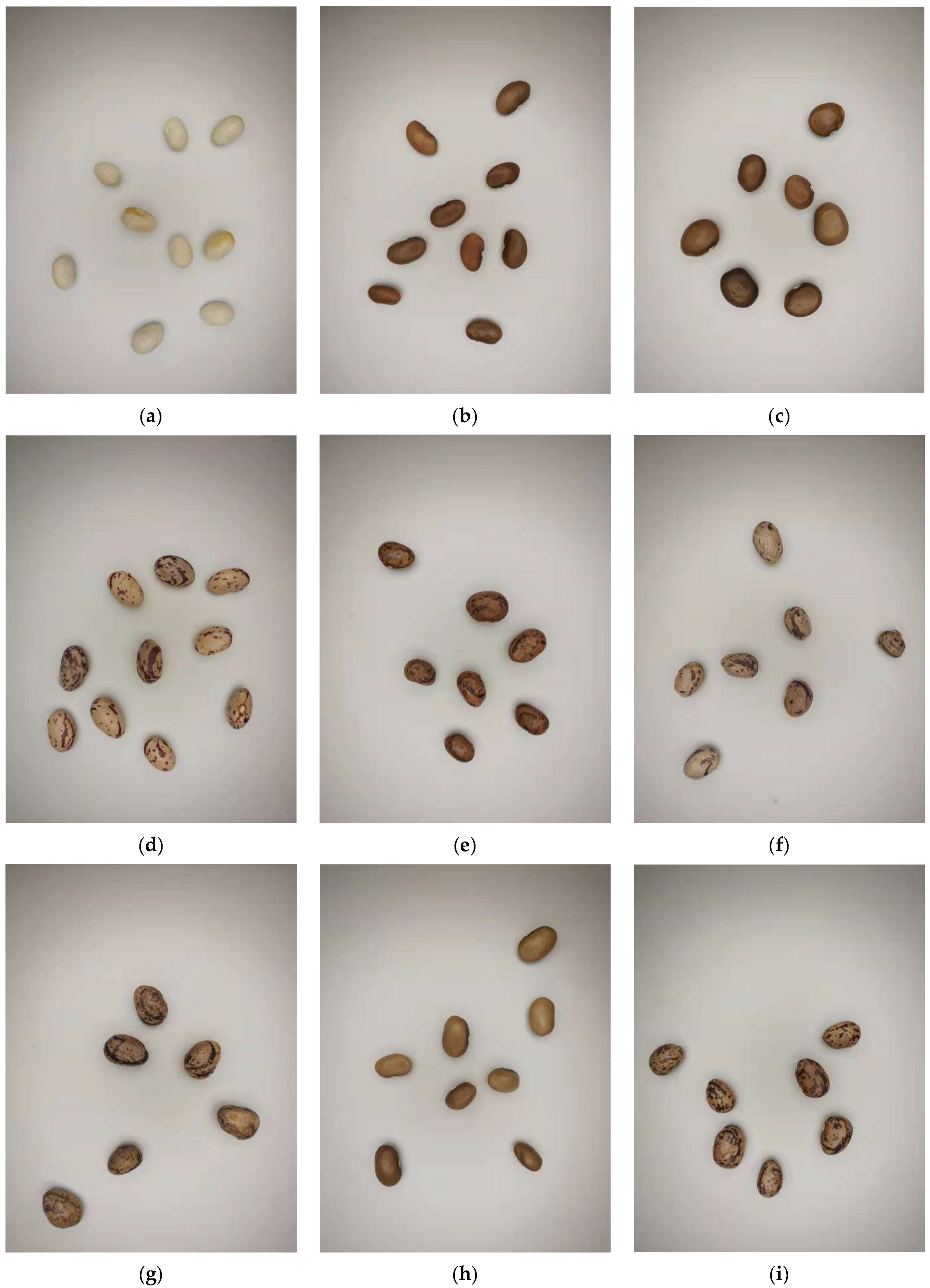
The image acquisition system is presented in Figure 1, which includes a mobile phone, a ring-light source with an adjustable light intensity, and seeds. The phone used was a Xiaomi MIX2. To mimic the light conditions on the assembly line, an LED ring-light source was placed at the center of the set-up. This way, the seeds could be imaged clearly. Additionally, it was ensured that the light intensity was constant via the use of a light-source controller. A cardboard box was placed around the equipment to prevent the interference of natural light. The whiteboard placed underneath the seeds was used to mimic the quality of the conveyor-belt device presenting a monotonous color. The phone was placed at a distance of about 10.5 cm from the whiteboard. Subsequently, 1292 images were captured, and the ratio of the training set to validation and test sets was 8:1:1. The environment was kept consistent while shooting was performed. The photographed seeds were not in contact with each other, as can be observed in Figure 2. In the dataset, each seed was captured once or twice. The dataset included images of one type of seed as shown in Figure 2a–j as well as the combinations of multiple types of seeds as shown in Figure 2k–m. The dataset had a resolution of 600 × 800 pixels and was saved in a “JPG” format. When the dataset was fed into the network, all the images were scaled to 416 × 416 pixels, which reduced the training time and memory usage. After the long side was scaled to 416 pixels, the short side was also scaled to the same multiple. The purpose of this was to prevent the distortion of the image and to accomplish equal scaling.
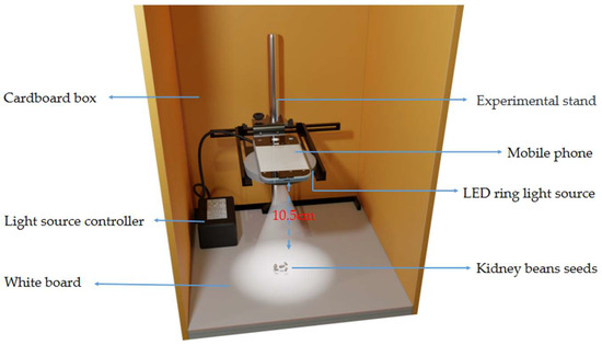
Figure 1.
The diagram of the image acquisition system.
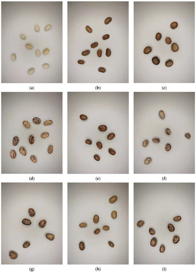
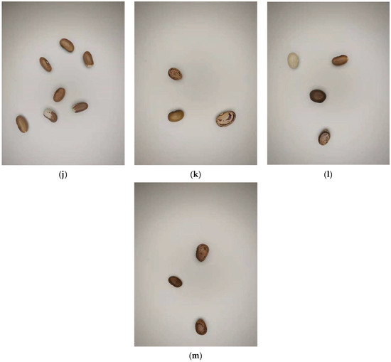
Figure 2.
The dataset of single-class and multi-class seeds: (a) bayuelv; (b) cuiguan; (c) dazihua; (d) fengguan; (e) hongguan; (f) jinguan; (g) juguan; (h) qingguan; (i) taikongdou; (j) yuguan; (k) combination of juguan, cuiguan, and hongguan seeds; (l) combination of taikongdou, qingguan, and fengguan; and (m) combination of bayuelv, yuguan, dazihua, and jinguan.
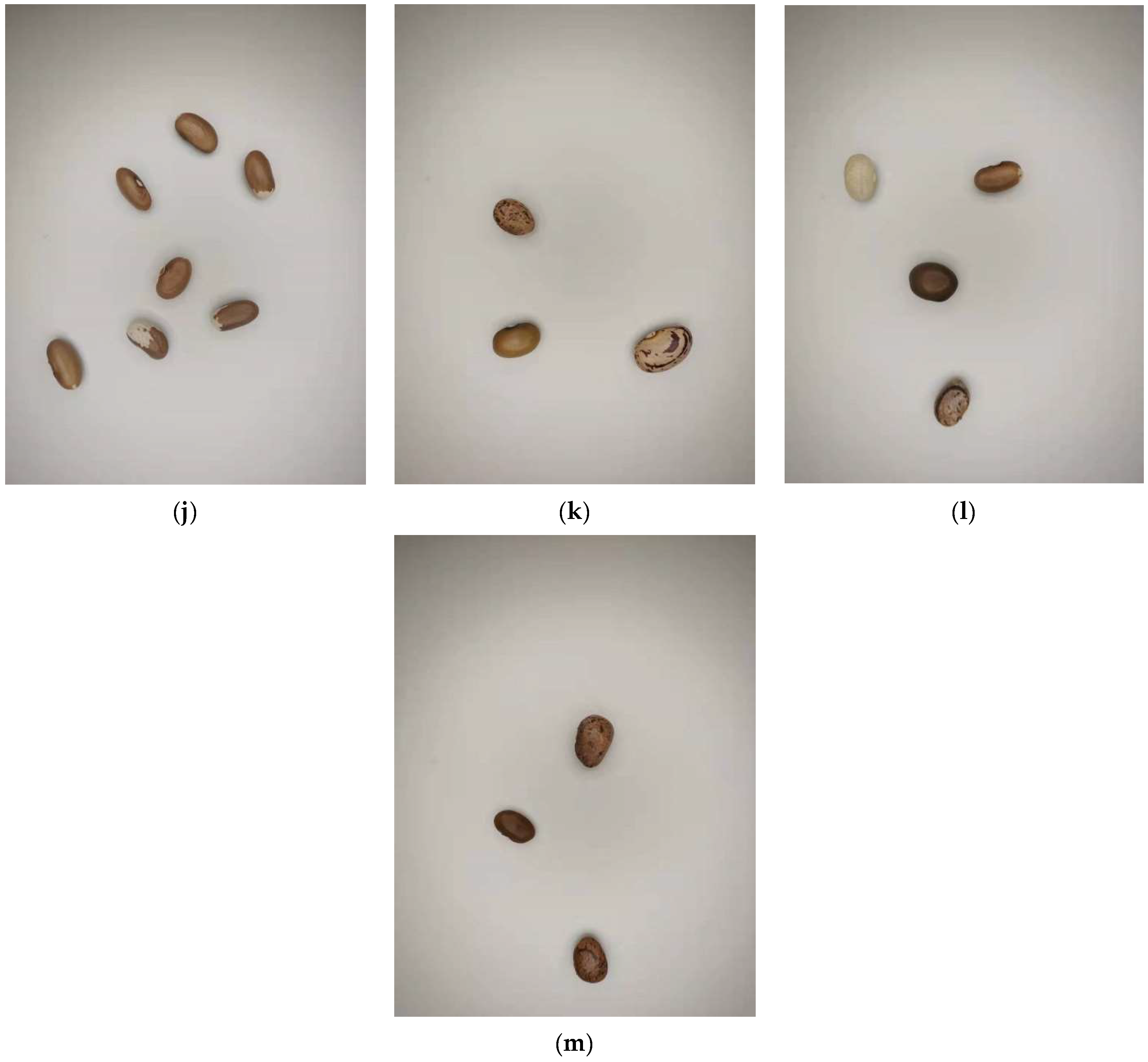
Different kinds of kidney bean seeds were labeled using the labeling tool LabelImg; the weights were obtained by training and testing according to the test set. The images of this dataset were processed into a JPG format, and the seeds of each species were labeled with the image processing tool LabelImg. Then, TXT files were generated by the LabelImg software to output the seed ID and coordinate location information, as presented in Figure 3. In Figure 3d, each row represents a seed that was labeled, and the labeled box was generated. From 0 to 3, the four categories of seeds were represented. The other four data in each row represent the center coordinates of the labeled box relative to the image, and the width and height of the labeled box relative to the image.
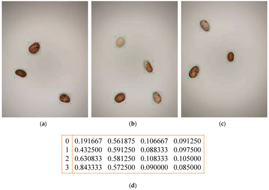
Figure 3.
Labeling diagram of seeds: (a–c) The results of ten types of seed labeling; (d) The ID and coordinate location information of kidney bean seeds in (b).
2.2. Yolov3 Network Structure
In the present study, a deep learning target detection algorithm was used to improve the efficiency of detection. It can detect multiple types of seeds simultaneously.
Yolo (You Only Look Once) is an end-to-end neural network, meaning that the image needs to be observed only once to obtain information about the target. Thus, it has been commonly used for target-detection practices [32]. The algorithm treats target detection as a regression problem in relation to target area and category predictions. The information about the position, size, and category of the target object in the image can be obtained. The Yolov3 model incorporates the advantages and disadvantages of other target-detection algorithms, such as SSD and Faster R-CNN. It is the same as the SSD algorithm in terms of detection accuracy, in comparison to other target-detection algorithms. However, the speed of detection is more advantageous than SSD and Faster R-CNN [33].
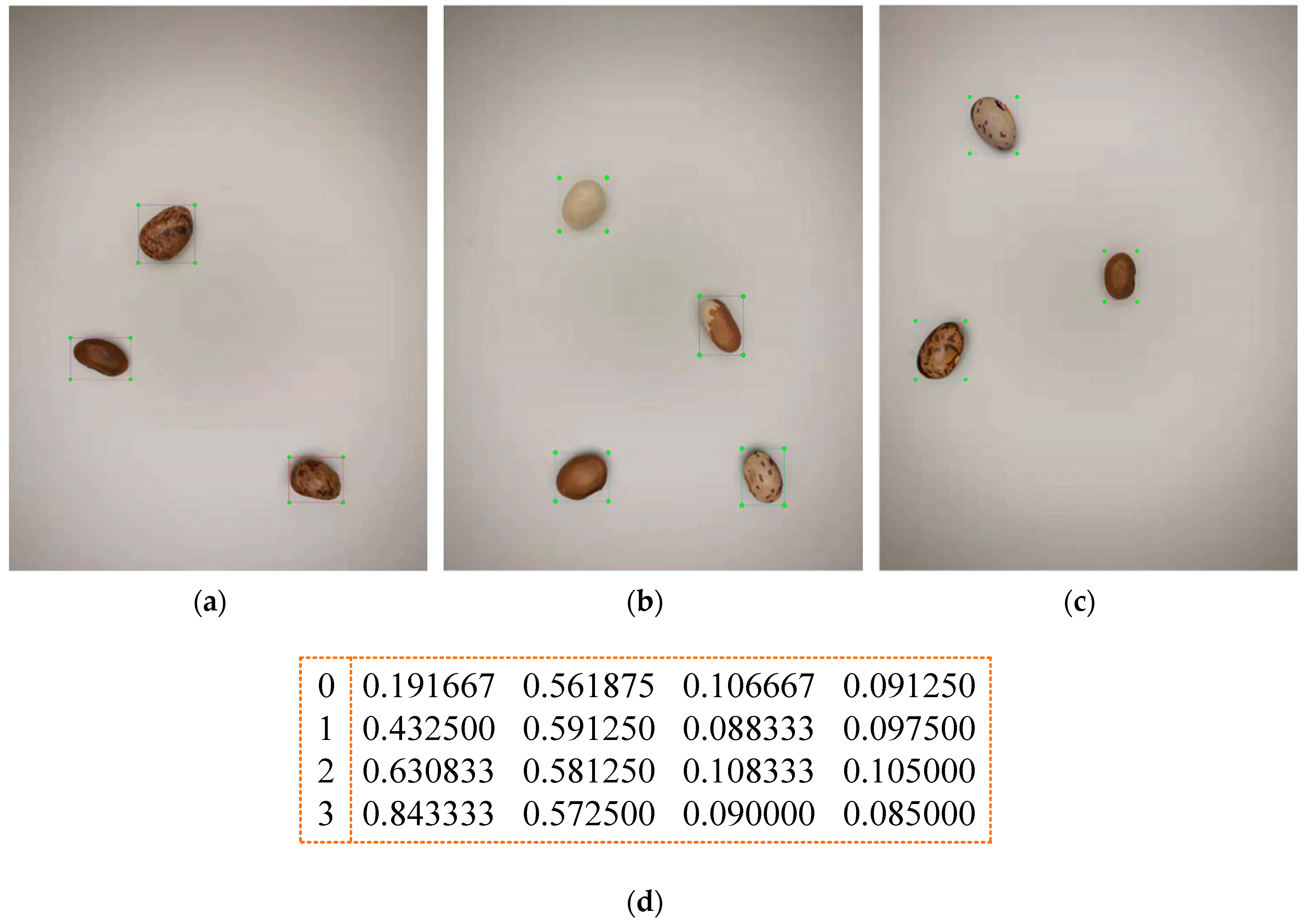
The network structure of Yolov3 is presented in Figure 4. The Yolov3 model is an improvement of the Yolov2 model, which mainly includes the optimization of the network structure. The Darknet19 network is improved in the Darknet53 network as the backbone network of the feature extractor, and multi-scale features are used for object detection [33]. The 52 convolutional layers were used to extract the features of the images in the network framework. To prevent the degradation of the model during the training of the deep network, Yolov3 created a link between the layers, which is borrowed from ResNet. The last layer is fully connected. Yolov3 could achieve localization and classification of targets in the images. The Darknet-53 network downsamples the image five times and also works with a residual net. This method allows the network to continue to rapidly converge in the deeper layers. Then, the features are extracted from the input image through a Yolo layer to obtain a feature map with a resolution of 13 × 13. The output feature map is upsampled by DBL operation on the 13 × 13 feature map, to obtain a 26 × 26 feature map. This is the same resolution as the feature map obtained by the five-times-downsampling strategy, and the results are summarized. Finally, the 26 × 26 feature map is upsampled and added to the feature map of the penultimate downsampling phase to obtain a 52 × 52 feature map [34]. In this way, the multi-scale prediction is achieved. The targets with different sizes can be predicted based on the different resolution feature maps. As presented in Figure 4, the Yolov3 network structure consists of three basic components: the CBL, Res unit, and ResX.

Figure 4.
The structure of the Yolov3 network.
CBL: This component consists of the Convolutional layer, BN layer, and Leaky Relu function.
Res unit: This component borrowed the residual structure from the Resnet network. This residual structure allows the network structure to converge even at very deep levels, and it allows the model to continue training.
ResX: This component consists of CBL and X residual components, which are the large components in Yolov3. The CBL component is used as a downsampling stage before each Res module. Each ResX contains 1 + 2 × X convolutional layers, so the entire backbone network contains a total of 52 convolutional layers.
As a lite version of the Yolov3 model, the Yolov3-tiny model has also been widely used with a quicker run speed. However, it may decrease the accuracy of detection. The backbone network consists of seven 3 × 3 convolutional layers and six pooling layers. The first 5 are pooling layers with a step size of 2. The last one is a pooling layer with a step size of 1. It also uses multiscale projections with resolutions of 26 × 26 and 13 × 13. For the same image, the detection result of Yolov3-tiny is weaker than Yolov3 in terms of position and confidence [35].
2.3. Yolov3 Model Compression
The actual online crop detection work often faces some hardware limitations [36]. Only simple and efficient algorithms can be more widely used in practical detection environments. Although the Yolov3 network can accurately detect kidney bean seeds, the Yolo network has a high number of parameters. Thus, it is necessary to compress the model. This is beneficial in a real-world-detection environment. Model pruning is a commonly used model compression method. It introduces sparsity to the dense links of deep neural networks. The number of non-zero weights was reduced by directly assigning zero values to the ‘unimportant’ weights.
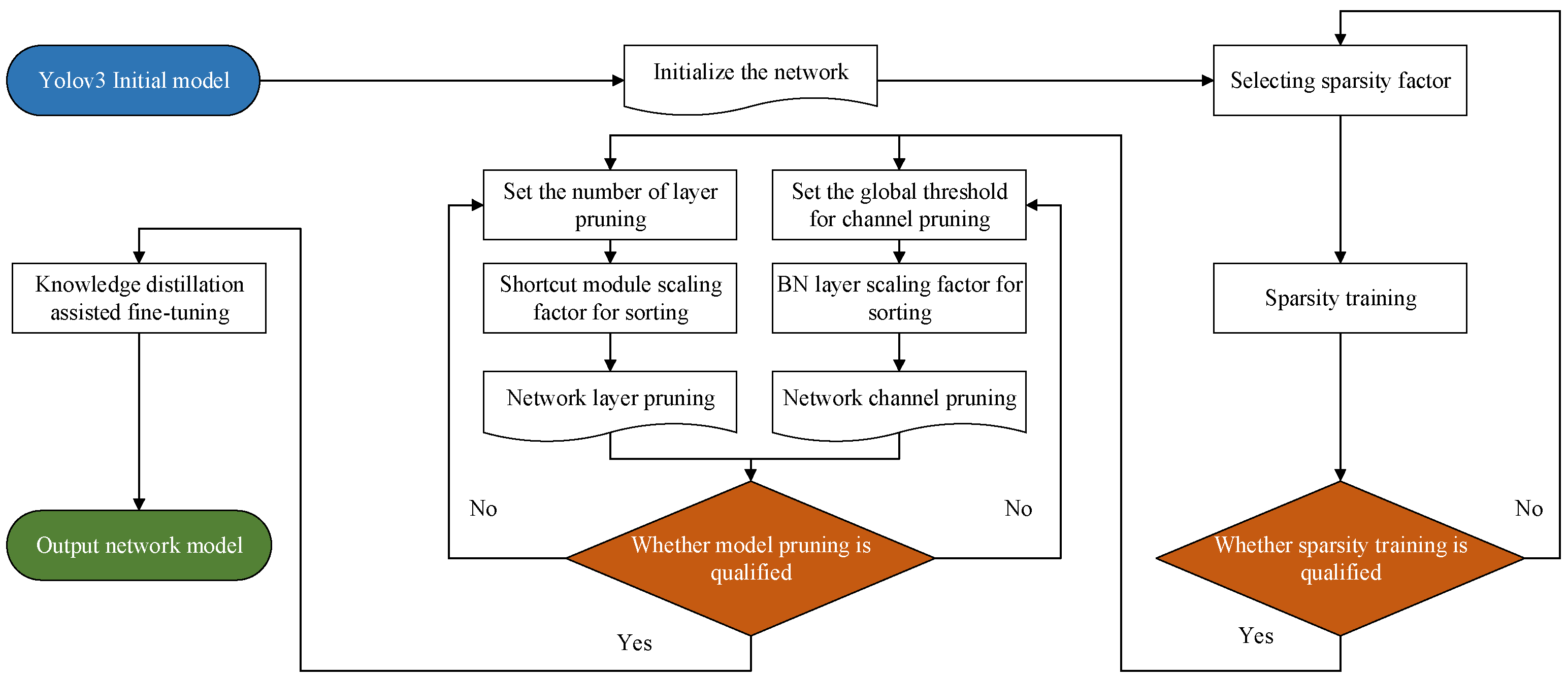
The model pruning method can be divided into four steps [37]: (1) analyzing the importance of each neuron in the trained model; (2) removing neurons with a low activation in the model for model inference; (3) fine-tuning the model to improve the accuracy of the pruned model; and (4) testing the fine-tuned model to determine whether the pruned model meets the requirements. The flow chart is presented in Figure 5.

Figure 5.
The flow chart for model compression.
2.3.1. Sparsity Training
Prior to pruning the Yolov3 model, it is necessary to detect the parts that are of least importance for the model. Therefore, sparsity training is required. Each convolutional layer in the Yolov3 network comes with a batch normalization layer, which enhances the convergence and generalization of the network. To obtain the importance scores, the scale factor in the batch-normalization layer is used as a measure of the importance of channels and layers. It simplifies the task of classifying neural networks [38].
The principle of the batch normalization layer is as follows: firstly, the mean and standard deviation of the output data in the previous layer is solved.
In Equations (1) and (2), m is the number of samples of images in one training process, i.e., the batch value. Following the normalization process, xi can be obtained. The batch normalization principle can adjust the training efficiency to prevent gradient explosion, etc.
In Equations (3) and (4), ε is an extremely small value added to prevent the denominator from being 0. γ is the scaling factor and β is the translation factor. In the current paper, γ is used as an important measure of the channel. The L1 parametric number is calculated by the γ of the channel, as shown in Equation (5):
The sparsity training loss function adds the regularization term to the Yolov3 loss function with the following Equation (6):
In summary, Lossyolo denotes the Yolov3 loss function, and s denotes the sparsity factor.
2.3.2. Model Pruning
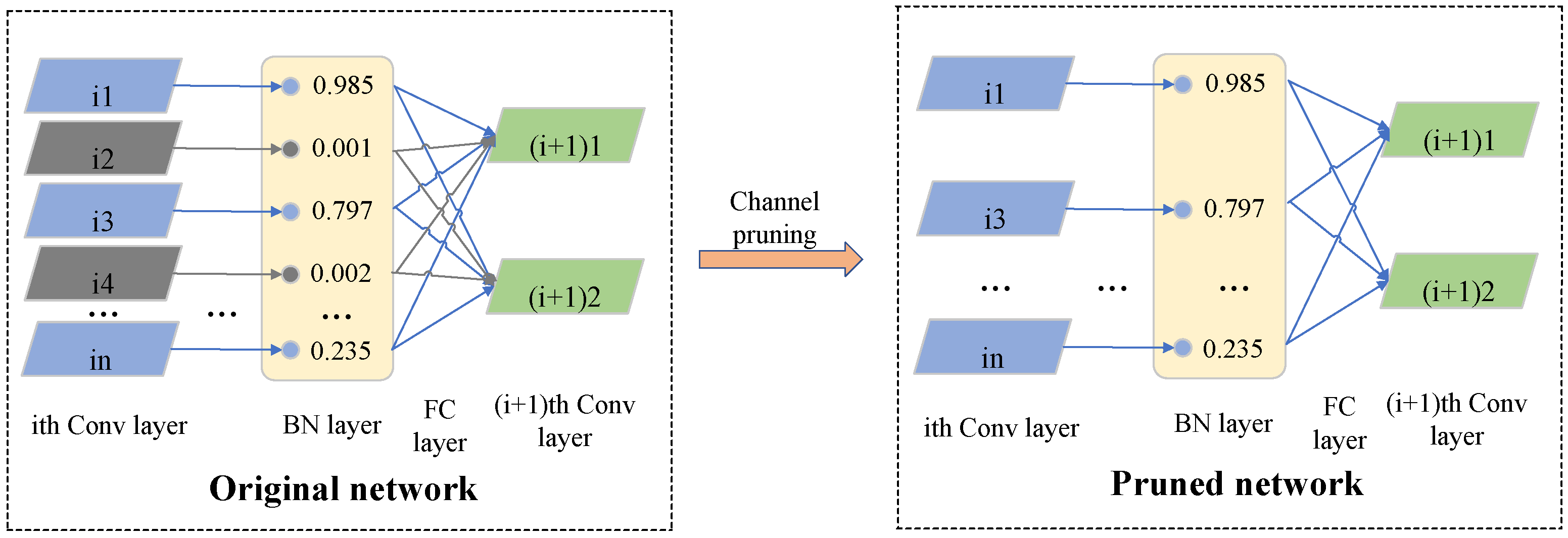
After the sparsity training, many scaling factors of the model were close to zero. Then, the sparsity scaling factor γ is ranked from smallest to largest. The closer the scaling factor is to zero, the less important the channel. Pruning the unimportant channels could simplify the model and reduce the model volume. The channel pruning process is presented in Figure 6. Therefore, the channels with scale factors close to zero, and the corresponding weights are pruned [39]. After sorting the scaling factors, ranging from small to large, the pruning rate needs to be set. The higher the pruning rate, the smaller the model size.

Figure 6.
The diagram for model pruning.
To ensure the integrity of the Yolov3 network structure, only the shortcut layers in the backbone network were pruned in the present study. The γ of each layer was ranked and the smallest value was used as the layer pruning.
2.3.3. Knowledge-Distillation Assisted Fine-Tuning
Large pruning leads to a considerable loss of model accuracy, so the pruned model needs to be fine-tuned. In the present study, knowledge distillation was used to fine-tune the model to improve the accuracy as much as possible. Knowledge distillation is based on the idea of transfer learning. More specifically, the student model was trained with the knowledge that was obtained from the relatively high-precision teacher model. This approach could accelerate the convergence of the student model [31]. Since the models have structural similarities both prior to and after pruning, they are well suited for fine-tuning with the help of knowledge distillation.
In traditional target-detection networks, the data are usually labeled with hard labels of “0” and “1”. However, hard labels contain limited information and do not include the relationship between classes. In contrast, knowledge distillation uses soft labels from the teacher network to label the data. The soft labels of the teacher network provide a considerable amount of information and can offer more information to the student network. This enables the more effective training of the student network as a way to improve the generalization ability of the model. Soft labels are present as probabilities in the category vector. The knowledge distillation algorithm introduces a temperature coefficient, T, in the softmax function. Appropriately increasing the value of T can result in a more even target category probability distribution; the information provided by the soft labels is amplified. In this way, the student model can focus more on the soft labels and further improve the training effect of the student model. The target category probability formula of the teacher network with the introduction of T is presented in Equation (7):
where vi is the output layer of the teacher model in class i, N is the total number of labels, and is the value of the soft label of the softmax function output of the teacher model in class i at a temperature of T.
Similarly, the target class probability formula for the student model network with the introduction of T is presented in Equation (8):
where zi is the output layer of the student model in class i, N is the total number of labels, and is the value of the soft label of the softmax function output of the student model in class i at a temperature of T. Similarly, in Equation (7) and in Equation (8) are used in Equations (9) to (11) to calculate the loss.
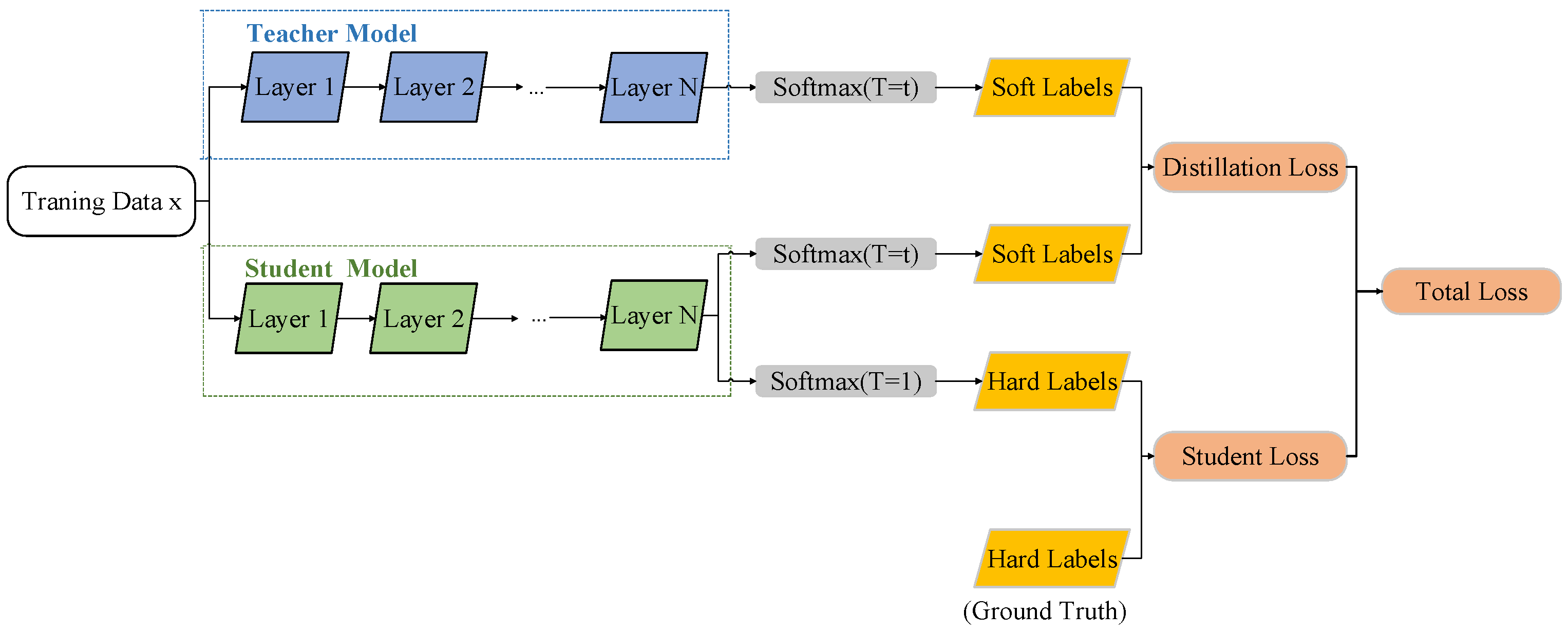
The flow of knowledge distillation is presented in Figure 7. The loss function is used to express the degree of difference between the prediction and actual data. It can measure how well the model performs predictions. It is obtained during the process of model training. Knowledge distillation is essentially also the process of training a model. Therefore, the loss of knowledge distillation needs to be calculated. Similarly, Figure 7 also illustrates the process of calculating the loss function for knowledge distillation. The loss function of knowledge distillation consists of two parts and the formula is as follows:
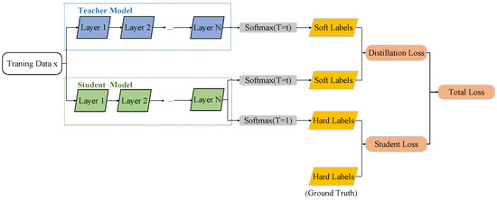
Figure 7.
The schematic of knowledge distillation.
The knowledge distillation loss is LossKD, which is obtained by weighting Losssoft and Losshard. The two weighting factors α and β have the sum of 1. In Figure 7, LossKD is the total loss, Losssoft is the distillation loss, and Losshard is the student loss.
For the input of the same dataset, the teacher and student models are subjected to the softmax layer to produce soft labels. At the same temperature, the cross-entropy loss function of the two soft labels is Losssoft. This part of the loss is the loss of information provided by the teacher model for the student model. The formula for Losssoft is as follows:
where and are the values of the soft labels presented in Equations (7) and (8), N is the total number of labels, and Losssoft is a fraction of the LossKD presented in Equation (9).
The cross-entropy loss between the output of softmax and ground truth is Losshard for the student model, under the condition that T is 1. The teacher model also has information about misclassification, and the error information received by the student model can be effectively reduced by introducing the ground truth value.
where is presented in Equation (8), ci is the ground truth value of class i, and Losshard is a fraction of LossKD presented in Equation (9).
3. Results
3.1. Parameter Settings and Hardware Conditions
Both the training and testing processes were implemented using a Windows 10 PC with the following specifications. The processor we used was AMD Ryzen 7 5800H with Radeon Graphics at 3.2 GHz, and the graphics card was NVIDIA GeForce RTX 3060 Laptop GPU with 6 GB of video memory size; the memory was 16 GB of RAM and 512 GB of SSD. The programming software used was PyCharm Community Edition 2021.3. The programming language was Python 3.8.12, and the training framework was Pytorch 1.7.0.
3.2. Model Evaluation Metrics
To verify the performance of the model, the following metrics were used to conduct the evaluation in the present paper. First, the loss function served as a measure of how well the model performs predictions. It represents the degree of difference between the predicted value and actual data. The smaller the loss function, the better the model is trained. The loss function of Yolov3 is presented in Equation (12):
where Lossyolo is the loss function of Yolov3; Lossobj is the confidence loss obtained from the model training process; Lossclass is the class loss obtained from the model training; Lossbox is the bounding box loss obtained from the model training; Lossyolo is the sum of Lossobj, Lossclass, and Lossbox.
The Precision is the accuracy rate, which indicates the number of correctly recognized objects as a percentage of the total number of recognized objects. It can be further understood how many of the samples with positive prediction results are positive samples. Precision is calculated, as presented in Equation (13):
where TP is the number of samples predicted to be positive, FP is the number of negative samples predicted to be positive, and the sum of TP and FP is the number of all samples predicted to be positive.
The Recall is the recall rate, which represents the percentage of the number of correctly identified objects compared to the total number of objects in the verification set. It can be understood further as how many positive cases in the sample are predicted correctly. Recall is calculated, as presented in Equation (14):
where FN is the number of samples that predict positive samples as negative. The sum of TP and FN represents the number of positive samples.
AP is the average precision of each category. AP is obtained by calculating the integral from Precision in Equation (13) and Recall in Equation (14). AP is often used to quantitatively measure the performance of the target detection model. The mAP is the average mean accuracy value presented for each category. The mAP is obtained by averaging the AP values of each category. The mAP is used to measure the accuracy of the target detection algorithm over the entire dataset. The higher the value of mAP, the better the model detection performance over the entire dataset. The mAP is the most important metric in the target detection algorithm. Therefore, mAP could be used as the main performance evaluation metric in the present paper. AP and mAP are calculated, as presented in Equations (15) to (16):
where c is the total number of categories.
3.3. The Result of Basic Training
The loss curve of the basic training is presented in Figure 8. The epochs of basic training were 100 in the current study.
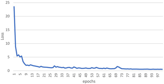
Figure 8.
The loss curve of basic training.
The learning rate was decreased 10 and 100 times at the 70th and 90th percentiles of the total training epochs, respectively. This caused the loss curves to converge more slowly. Therefore, they became more stable at the 70th and 90th percentiles of the total training epoch.
Figure 8 shows that the initial stage of model training is more efficient for learning, which results in a more rapid convergence of the curve. As the learning rate decreases, the trained model tends to gradually become stable. Following 100 epochs, the training loss was stabilized at 0.5240.
3.4. Effect of Model Compression on Model Performance
3.4.1. Selection of the Sparsity Factor
To finally achieve a tight network, a suitable sparsity factor first needs to be found. It not only ensures that the loss of the model following sparsity training is minimal, but also ensures that the mAP of the final compressed model does not decrease too considerably.
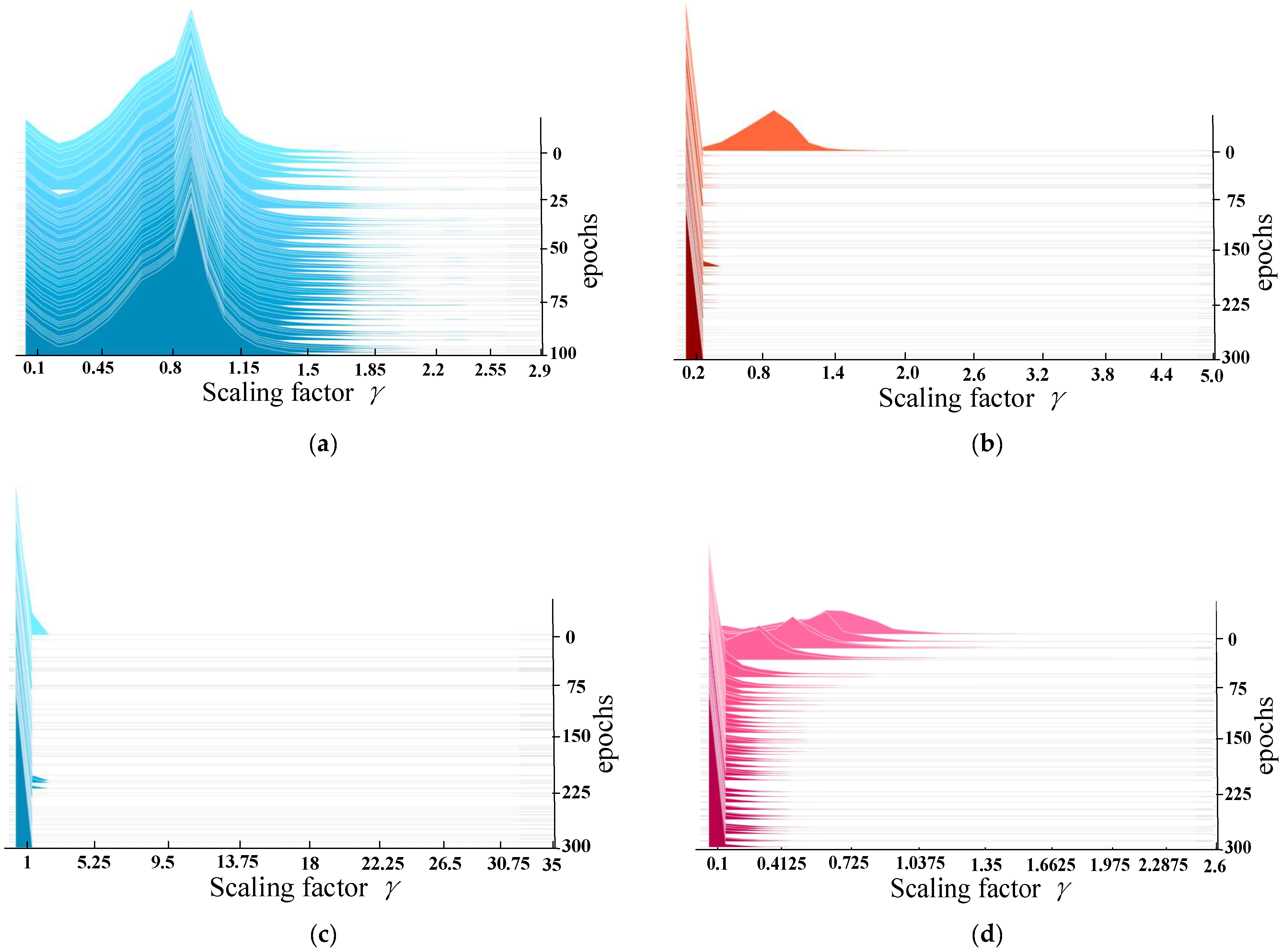
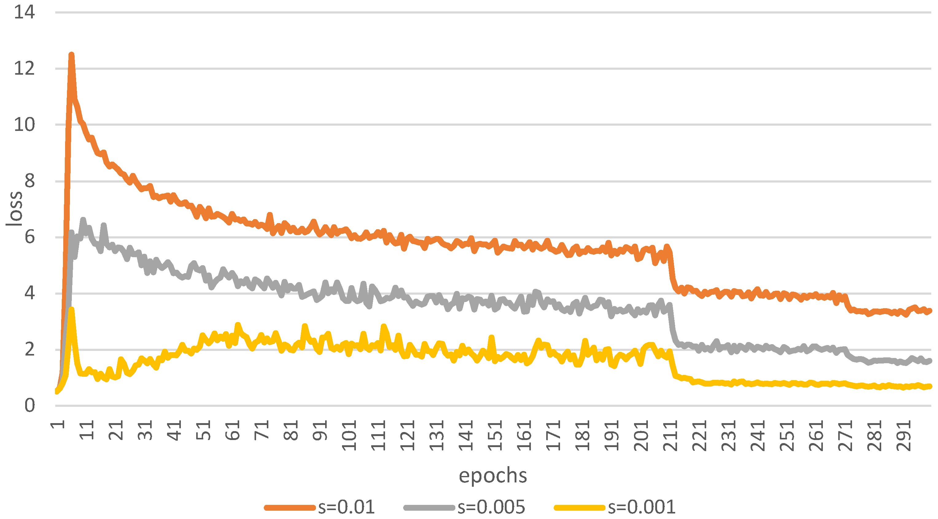
The sparsity factors used in this study were 0.01, 0.005, and 0.001 for 300 epochs. The epochs of basic training without sparsity training were 100. The scale factor without sparsity training approximated a normal distribution with a value of 1.
Figure 9 presented the changes in the scale factor prior to and after sparsity training. Additionally, the model obtained by choosing different sparsity factors, s, for sparsity training is presented in Figure 9. It can be observed that scaling factor γ of the sparsely trained model tends to be close to 0. Scaling factor γ close to 0 corresponds to channels with lower-weight. The importance of the less weight channels is low, so they should be pruned. At sparsity factors of 0.01 and 0.001 and training 300 epochs, the value of the scaling factor is close to 0. Therefore, there were fewer weight channels in the network.
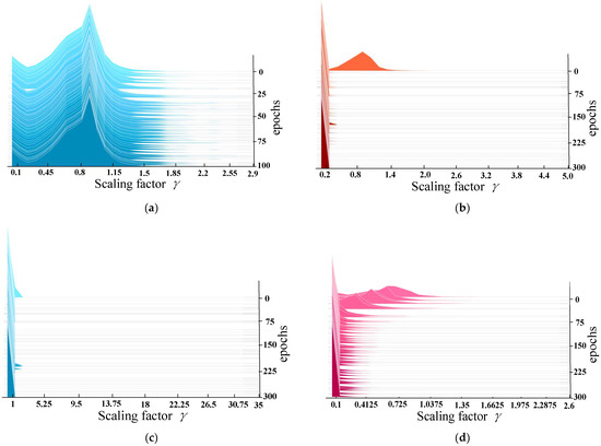
Figure 9.
(a) Histogram of the distribution of scaling factors of the BN layer for basic training prior to sparsity training (b–d). Histograms of the distribution of the BN layer scaling factors for sparsity training, with sparsity factors of 0.01, 0.005, and 0.001.
Additionally, it can be observed in Figure 10 that the lowest model training loss is obtained when the sparsity factor takes the value of 0.001. Thus, the model with the sparsity factor of 0.001 was pruned in the present study. The sparsity factor here was s in the regularization term in Equation (6). In summary, the model with a sparsity factor of 0.001 was pruned in the current study.
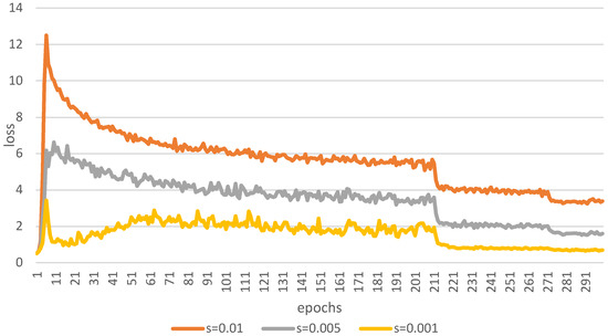
Figure 10.
The loss curve for sparsity training with different sparsity factors.
3.4.2. Model Pruning Comparison
After the sparsity factor s = 0.001 was determined, the Yolov3 network was pruned with channels and layers. The purpose of pruning was to reduce the inference time of the model without significantly degrading the model’s performance. To obtain the most concise model, the pruning rate was set in an incremental way, starting from 0, with an interval of 0.1. Since the mAP of the model did not dramatically decrease at a pruning rate of 0.9, the pruning rate was continued in an incremental way, starting from 0.9 with an interval of 0.01 to simplify the model further. By using this method, the maximum pruning rate could be found, which resulted in the most concise model. Meanwhile, only 16 shortcut layers were pruned to ensure the integrity of the model’s structure.
The mAP of the model prior to pruning was 99.19%, the inference time was 16.9 ms, and the size of the model was 235 MB.
Since the layers were pruned at the same time as the pruned channels, the performance of the model changed when the pruning rate was 0. It can be observed from Table 1 that the mAP of the model does not drastically decrease from 0 to 0.93, and the model mAP can be recovered by performing fine-tuning. Meanwhile, the inference time and size of the model decreased with the increase in the pruning rate; thus, the inference cost of the model also decreases. The mAP of the model decreased to 0 when the pruning rate was 0.94. This was because too large a pruning rate removes too much of scale factor γ. γ is close, but not equal, to 0. Thus, there was no requirement to set a pruning rate greater than 0.94. In summary, a pruning rate of 0.93 was finally selected.

Table 1.
The comparison of different pruning rate parameters.
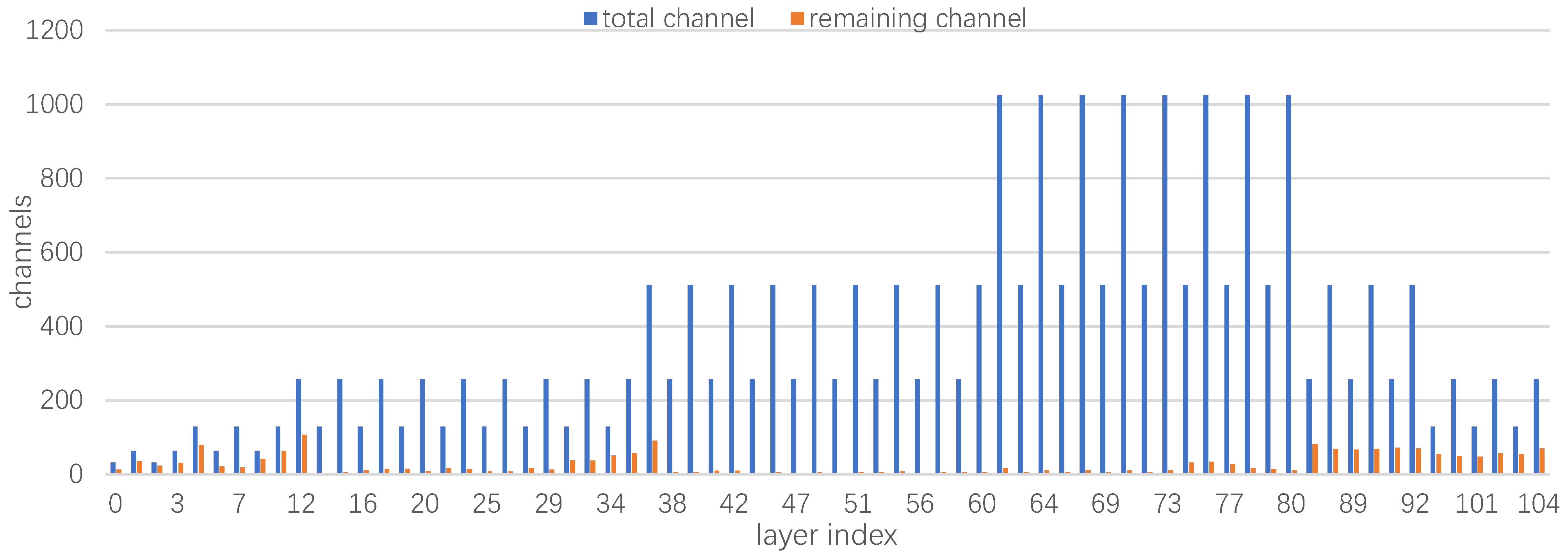
Figure 11 presents the change in channels following pruning; it can be observed that the channels are significantly reduced, especially channels 38 to 73. It can also be observed that some layer indexes of the network were lost, which indicates that the shortcut layers of the network were also successfully pruned. The Yolo pruning algorithm can significantly reduce the computational effort of the network model. Therefore, the method was feasible.
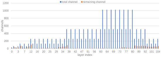
Figure 11.
The changes of channels in each layer of the Yolov3 network prior to and after pruning.
3.4.3. Knowledge Distillation Fine-Tuning Comparison
In the current study, the pruned model was fine-tuned using a knowledge distillation strategy with 50 epochs, and the distillation temperature T was set to 3.0. The selected teacher network model was the network model, which incorporated basic training without the use of model compression. The student network model we selected was the pruned network model, which set the pruning rate as 0.93.
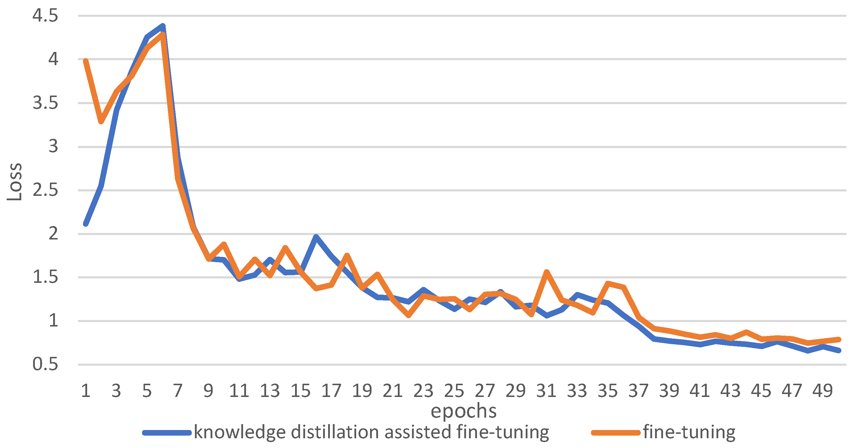
The mAP of knowledge-distillation-assisted fine-tuning and fine-tuning are presented in Figure 12. The loss functions of knowledge-distillation-assisted fine-tuning and fine-tuning are presented in Figure 13.
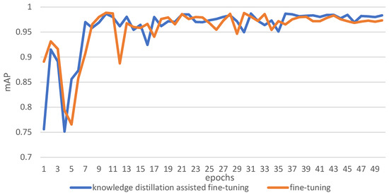
Figure 12.
The comparison of the mAP of fine-tuning and knowledge-distillation-assisted fine-tuning.
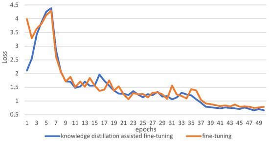
Figure 13.
The comparison of the loss of fine-tuning and knowledge-distillation-assisted fine-tuning.
The model stabilized at 39–49 epochs. During these epochs, the mAP was greater as a result of using the knowledge distillation method of fine-tuning with a lower loss of training.
3.4.4. Comparison of Object Detection Models
To compare the speed and accuracy, the present study compared the Yolov3 network, pruned Yolov3 network, Yolov3-tiny network, and Yolov4 network in terms of recall, precision, mAP, model size, and inference time. The results are presents in Table 2.
Table 2.
The performance comparison of different networks.
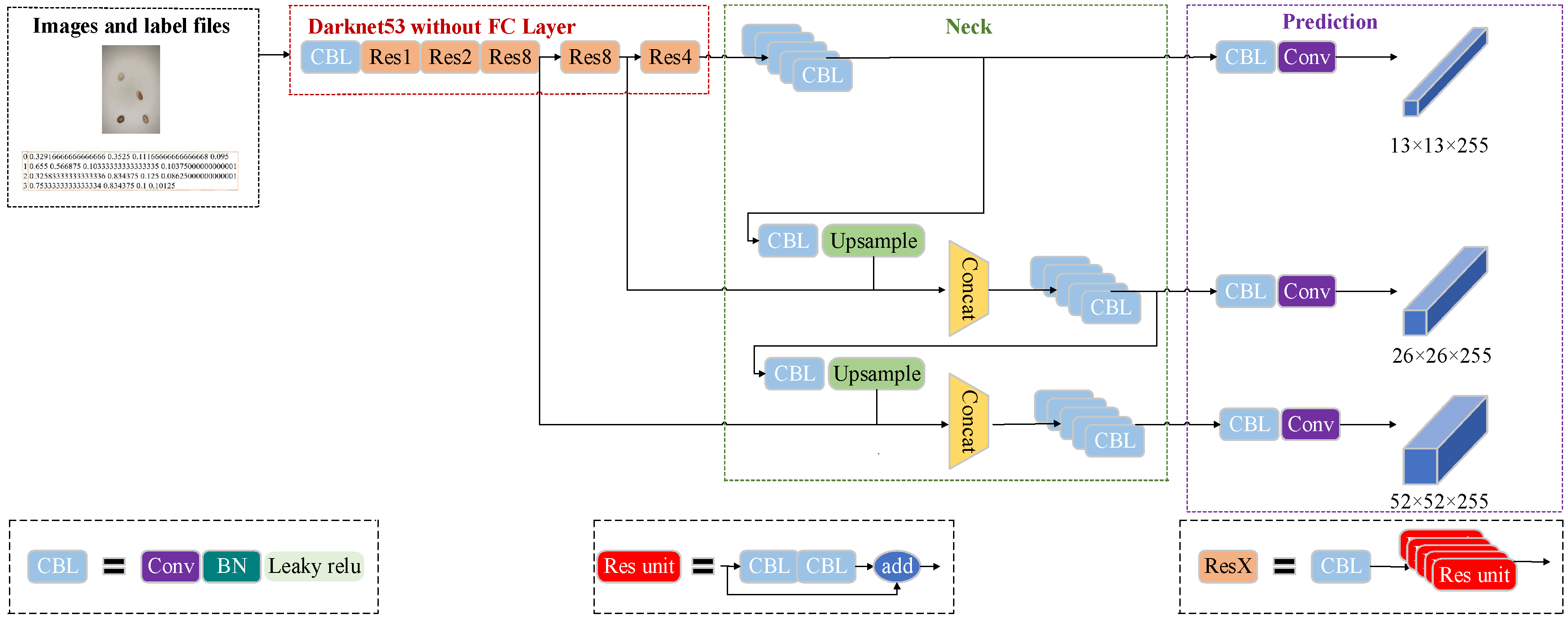
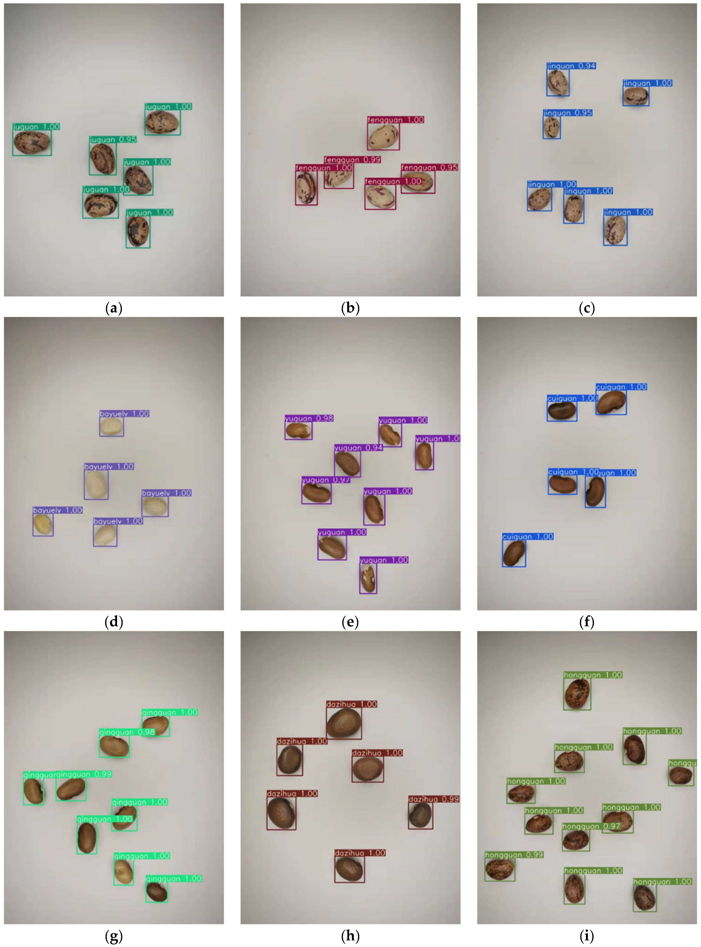
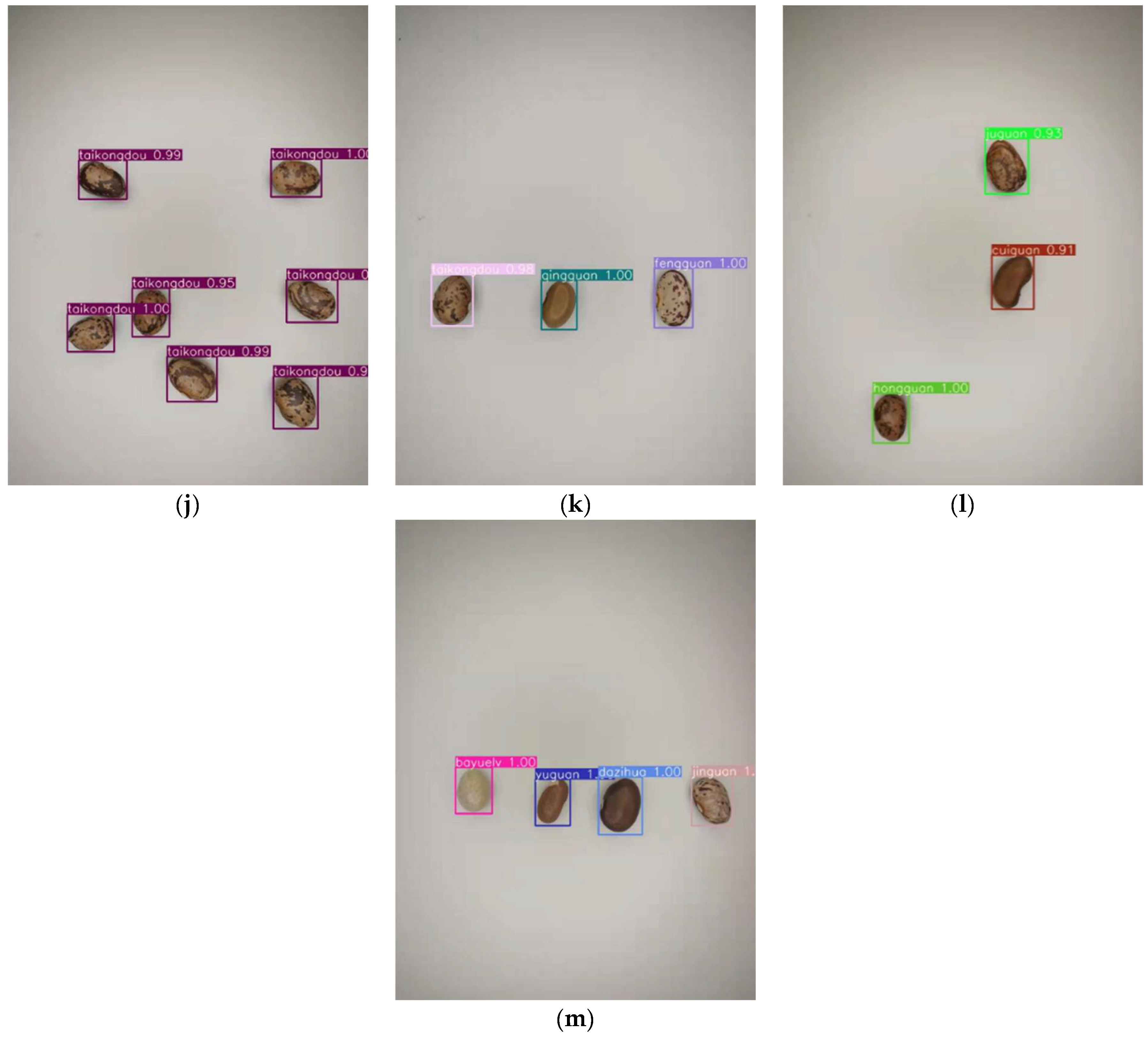
It can be seen observed that the pruning network reduces the inference time from 16.9 to 6.6 ms. In comparison to the Yolov3 network, the inference time is reduced by 2.56 times. The network used in this study was also faster than Yolov4. The mAP was 1.37% higher than Yolov3-tiny. Some of the detection results are presented in Figure 14.

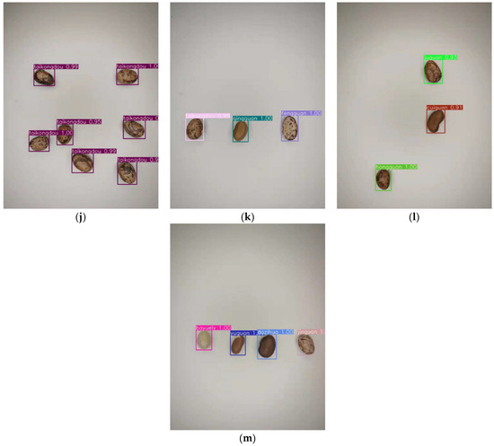
Figure 14.
(a–j) The detection results for ‘juguan’, ‘fengguan’, ‘jinguan’, ‘bayuelv’, ‘yuguan’, ‘cuiguan’, ‘qingguan’, ‘dazihua’, ‘hongguan’, and ‘taikongdou’. (k–m) The detection results for random combinations of different classes of seeds.
4. Discussion
The mAP achieved 99.19% during the basic training phase. In this way, the model can focus more on the feature information of the seeds during the training process. In the process of sparsity training, different sparsity factors were chosen, and the results obtained for the sparsity training were different. By using sparsity factors, s, of 0.01 and 0.005, the scaling factor γ of the BN layer was rapidly compressed. By using a sparsity factor s, of 0.001, the scaling factor γ of the BN layer was compressed more slowly. Sparsity training using sparsity factors, s, of 0.01 and 0.001 after 300 epochs meant that the scale factor γ could be compressed to a value close to 0. Therefore, an insignificant part of the network was revealed. However, the sparsity factor s of 0.001 ensured a lower loss value, which allowed the model to be trained in a more efficient manner. In the process of pruning, a pruning rate of 0.93 was selected in the study to reduce the unimportant parameters of the model as much as possible. If the pruning rate was increased further, the mAP of the model would be completely lost. This is because too much scaling factor was pruned out, which was close but not equal to 0; it is difficult to make the model mAP recover by fine-tuning methods when using pruning rates that are too high. Finally, the knowledge distillation algorithm was introduced in the fine-tuning process. The pruned model was made to obtain the help of the teacher model. The pruned model obtained more information from the soft labels of the teacher model. Thus, using knowledge distillation to assist in the fine-tuning process can cause the model mAP to increase further. The Yolov3 network was completed using compression. Finally, the improved network used in the present study was compared to the Yolov3, Yolov4 and Yolov3-tiny networks. By comparing it to other networks, it was determined that the improved network had advantages in both speed and accuracy.
In future short-term plans, the research will focus on the following factors. (1) Adding different combinations of seeds, and using different light-intensity adjustments. These methods will be used to enrich the dataset as a way to improve the generalization ability of the model. (2) Deploying the trained models in embedded devices to form a highly portable, low-power, low-cost detection system. (3) Replace the lightweight backbone network by employing model quantization to obtain a microscopic model. Ensuring accuracy while reducing the model’s inference time is also an aspect on which the present study will focus in the future.
5. Conclusions
The current paper addressed the problem of the detection of kidney bean seeds. The mAP for basic training reached 99.19%. In real-world detection, not only does the accuracy of detection need to be high, but the speed of detection also needs to be rapid. To reduce the computational cost in the actual detection environment, the Yolov3 model was pruned, and then the pruned network was fine-tuned by knowledge distillation. The experimental results show that the method utilized in the present study significantly reduces both the model’s parameters and resource consumption with guaranteed accuracy. The accuracy was higher than that produced by Yolov3-tiny, reaching 98.33%. The detection time was reduced from 16.2 to 6.6 ms, with a speedup of 2.56 times. Meanwhile, the model size was reduced from 235 to 4.07 M, with a compression rate of 98%. The obtained model met the requirement for the rapid and accurate detection of kidney bean seeds.
Author Contributions
Conceptualization, Y.W., H.B. and L.S.; methodology, Y.W.; software, Y.W.; validation, Y.W.; formal analysis, Y.W.; investigation, Y.W., Y.T. and Y.H.; resources, H.B.; data curation, Y.W.; writing—original draft preparation, Y.W.; writing—review and editing, Y.W., H.B. and R.M.; visualization, Y.W.; supervision, H.B.; project administration, Y.W.; funding acquisition, H.B. All authors have read and agreed to the published version of the manuscript.
Funding
This research was funded by the Heilongjiang Provincial Natural Science Foundation of China (SS2021C005, F2018026), University Nursing Program for Young Scholars with Creative Talents in Heilongjiang Province (UNPYSCT-2018012), and Fundamental Research Funds for the Heilongjiang Provincial Universities (KJCXZD201703).
Institutional Review Board Statement
Not applicable.
Informed Consent Statement
Not applicable.
Data Availability Statement
Not applicable.
Conflicts of Interest
The authors declare no conflict of interest.
References
- Tu, K.; Wen, S.; Cheng, Y.; Zhang, T.; Pan, T.; Wang, J.; Wang, J.; Sun, Q. A Non-Destructive and Highly Efficient Model for Detecting the Genuineness of Maize Variety ‘JINGKE 968′ Using Machine Vision Combined with Deep Learning. Comput. Electron. Agric. 2021, 182, 106002. [Google Scholar] [CrossRef]
- Cui, Y.; Xu, L.; An, D.; Liu, Z.; Gu, J.; Li, S.; Zhang, X.; Zhu, D. Identification of Maize Seed Varieties Based on near Infrared Reflectance Spectroscopy and Chemometrics. Int. J. Agric. Biol. Eng. 2018, 11, 177–183. [Google Scholar] [CrossRef]
- Risheh, A.; Tavakolian, P.; Melinkov, A.; Mandelis, A. Infrared computer vision in non-destructive imaging: Sharp delineation of subsurface defect boundaries in enhanced truncated correlation photothermal coherence tomography images using K-means clustering. NDT E Int. 2022, 125, 102568. [Google Scholar] [CrossRef]
- Kiani, S.; Minaei, S.; Ghasemi-Varnamkhasti, M. Integration of computer vision and electronic nose as non-destructive systems for saffron adulteration detection. Comput. Electron. Agric. 2021, 182, 106054. [Google Scholar] [CrossRef]
- Palumbo, M.; Pace, B.; Cefola, M.; Montesano, F.F.; Colelli, G.; Attolico, G. Non-destructive and contactless estimation of chlorophyll and ammonia contents in packaged fresh-cut rocket leaves by a Computer Vision System. Postharvest Biol. Technol. 2022, 189, 111910. [Google Scholar] [CrossRef]
- Wei, Y.; Li, X.; Pan, X.; Li, L. Nondestructive Classification of Soybean Seed Varieties by Hyperspectral Imaging and Ensemble Machine Learning Algorithms. Sensors 2020, 20, 6980. [Google Scholar] [CrossRef]
- Ahmed, M.R.; Yasmin, J.; Yasmin, J.; Park, E.; Kim, G.; Kim, M.S.; Wakholi, C.; Mo, C.; Cho, B.K. Classification of Watermelon Seeds Using Morphological Patterns of X-ray Imaging: A Comparison of Conventional Machine Learning and Deep Learning. Sensors 2020, 20, 6753. [Google Scholar] [CrossRef]
- Ma, T.; Tsuchikawa, S.; Inagaki, T. Rapid and non-destructive seed viability prediction using near-infrared hyperspectral imaging coupled with a deep learning approach. Comput. Electr. Eng. 2020, 177, 105683. [Google Scholar] [CrossRef]
- Krizhevsky, A.; Sutskever, I.; Hinton, G.E. ImageNet Classification with Deep Convolutional Neural Networks. Adv. Neural. Inf. Process. Syst. 2012, 25, 2. [Google Scholar] [CrossRef]
- Xu, P.; Tan, Q.; Zhang, Y.; Zha, X.; Yang, S.; Yang, R. Research on Maize Seed Classification and Recognition Based on Machine Vision and Deep Learning. Agriculture 2022, 12, 232. [Google Scholar] [CrossRef]
- Jin, S.; Zhang, W.; Yang, P.; Zheng, Y.; An, J.; Zhang, Z.; Qu, P.; Pan, X. Spatial-spectral feature extraction of hyperspectral images for wheat seed identification. Comput. Electr. Eng. 2022, 101, 108077. [Google Scholar] [CrossRef]
- Andrea, L.; Mauro, L.; Cecelia, D.R. A novel deep learning based approach for seed image classification and retrieval. Comput. Electron. Agric. 2021, 187, 106269. [Google Scholar]
- Helizani, C.B.; José, P.M.; Daniel, A.; Maurício, M. Detection, classification, and mapping of coffee fruits during harvest with computer vision. Comput. Electron. Agric. 2021, 183, 106066. [Google Scholar]
- Islam, M.K.; Habiba, S.U.; Ahsan SM, M. Bangladeshi Plant Leaf Classification and Recognition Using YOLO Neural Network. In Proceedings of the 2019 2nd International Conference on Innovation in Engineering and Technology (ICIET), Dhaka, Bangladesh, 23–24 December 2019; pp. 1–5. [Google Scholar]
- Yuan, X. Image multi-target detection and segmentation algorithm based on regional proposed fast intelligent network. Cluster. Comput. 2019, 22, S3385–S3393. [Google Scholar] [CrossRef]
- Huang, P.; Liu, S.; Wang, Z.; Ding, T.; Xu, Y. Deriving the predicted no effect concentrations of 35 pesticides by the QSAR-SSD method. Chemosphere 2022, 298, 134303. [Google Scholar] [CrossRef]
- Li, Z.; Li, Y.; Yang, Y.; Guo, R.; Yang, J.; Yue, J.; Wang, Y. A high-precision detection method of hydroponic lettuce seedlings status based on improved Faster RCNN. Comput. Electron. Agric. 2021, 182, 106054. [Google Scholar] [CrossRef]
- Li, Y.; Li, M.; Qi, J.; Zhou, D.; Zou, Z.; Liu, K. Detection of typical obstacles in orchards based on deep convolutional neural network. Comput. Electron. Agric. 2021, 181, 105932. [Google Scholar] [CrossRef]
- Gao, Z.; Yao, Y.; Wei, X.; Yan, T.; Zeng, S.; Ge, G.; Wang, Y.; Ulah, A.; Reviriego, P. Reliability evaluation of FPGA based pruned neural networks. Microelectron. Reliab. 2022, 130, 114498. [Google Scholar] [CrossRef]
- Li, Y.; Li, K.; Liu, X.; Wang, Y.; Zhang, L. Lithium-ion battery capacity estimation—A pruned convolutional neural network approach assisted with transfer learning. Appl. Energy 2021, 285, 116410. [Google Scholar] [CrossRef]
- Hashmi, A.S.; Ahmad, T. GP-ELM-RNN: Garson-pruned extreme learning machine based replicator neural network for anomaly detection. J. King Saud Univ.-Comput. Inf. Sci. 2022, 34, 1768–1774. [Google Scholar] [CrossRef]
- Choudhary, T.; Mishra, V.; Goswami, A.; Sarangapani, J. A transfer learning with structured filter pruning approach for improved breast cancer classification on point-of-care devices. Comput. Biol. Med. 2021, 134, 104432. [Google Scholar] [CrossRef]
- Li, Z.; Lei, X.; Liu, S. A lightweight deep learning model for cattle face recognition. Comput. Electron. Agric. 2022, 195, 106848. [Google Scholar] [CrossRef]
- Das, P.K.; Nayak, B.; Meher, S. A lightweight deep learning system for automatic detection of blood cancer. Measurement 2022, 191, 110762. [Google Scholar] [CrossRef]
- Chen, K.; Zhang, Y. Real-time ship detection in satellite images based on YOLO-v3 model compression. Chin. J. Liq. Cryst. Disp. 2020, 35, 1168–1176. [Google Scholar] [CrossRef]
- Wu, D.; Lyu, S.; Jiang, M.; Song, H. Using channel pruning-based YOLO v4 deep learning algorithm for the real-time and accurate detection of apple flowers in natural environments. Comput. Electron. Agric. 2020, 178, 105742. [Google Scholar] [CrossRef]
- Ni, J.; Li, J.; Deng, L.; Han, Z. Intelligent detection of appearance quality of carrot grade using knowledge distillation. Trans. Chin. Soc. Agric. Eng. 2020, 36, 181–187. [Google Scholar]
- Cao, S.; Zhao, D.; Liu, X.; Sun, Y. Real-time robust detector for underwater live crabs based on deep learning. Comput. Electron. Agric. 2020, 172, 105339. [Google Scholar] [CrossRef]
- Wei, W.; Gu, H.; Deng, W.; Xiao, Z.; Ren, X. ABL-TC: A lightweight design for network traffic classification empowered by deep learning. Neurocomputing 2022, 489, 333–334. [Google Scholar] [CrossRef]
- Jordao, A.; Lie, M.; Schwartz, W.R. Discriminative layer pruning for convolutional neural networks. IEEE J. Sel. Top. Signal. Process. 2020, 14, 828–837. [Google Scholar] [CrossRef]
- Chen, L.; Chen, Y.; Xi, J.; Le, X. Knowledge from the original network: Restore a better pruned network with knowledge distillation. Complex. Intell. Syst. 2021, 8, 709–718. [Google Scholar] [CrossRef]
- Redmon, J.; Divvala, S.; Girshick, R.; Farhadi, A. You only look once: Unified, Real-time object detection. In Proceedings of the IEEE Conference on Computer Vision and Pattern Recognition (CVPR), Las Vegas, NV, USA, 27–30 June 2016; pp. 779–788. [Google Scholar]
- Redmon, J.; Farhadi, A. Yolov3: An Incremental Improvement. In Proceedings of the 2018 IEEE Conference on Computer Vision and Pattern Recognition, Salt Lake City, UT, USA, 18–23 June 2018; pp. 1–6. [Google Scholar]
- Won, J.H.; Lee, D.H.; Lee, K.M.; Lin, C.H. An Improved Yolov3-based Neural Network for De-identification Technology. In Proceedings of the 2019 34th International Technical Conference on Circuits/Systems, Computers and Communications (ITC-CSCC), Seogwipo, Korea, 23–26 June 2019; pp. 1–2. [Google Scholar]
- Fu, L.; Feng, Y.; Wu, J.; Liu, Z.; Gao, F.; Majeed, Y.; Al-Mallahi, A.; Zhang, Q.; Li, R.; Cui, Y. Fast and accurate detection of kiwifruit in orchard using improved YOLOv3-tiny model. Precis. Agric. 2020, 22, 754–776. [Google Scholar] [CrossRef]
- Song, S.; Liu, T.; Wang, H.; Hasi, B.; Yuan, C.; Gao, F.; Shi, H. Using Pruning-Based YOLOv3 Deep Learning Algorithm for Accurate Detection of Sheep Face. Animals 2022, 12, 1465. [Google Scholar] [CrossRef]
- Zhang, P.; Zhong, Y.; Li, X. SlimYOLOv3: Narrower, faster and better for real-time UAV applications. In Proceedings of the 2019 IEEE/CVF International Conference on Computer Vision Workshop (ICCVW), Seoul, Korea, 27–28 October 2019; pp. 37–45. [Google Scholar]
- Ioffe, S.; Szegedy, C. Batch normalization: Accelerating deep network training by reducing internal covariate shift. In Proceedings of the 32nd International Conference on International Conference on Machine Learning (ICML), Lille, France, 6–11 July 2015; pp. 448–456. [Google Scholar]
- Molchanov, P.; Mallya, A.; Tyree, S. Importance Estimation for Neural Network pruning. In Proceedings of the 2019 IEEE/CVF Conference on Computer Vision and Pattern Recognition (CVPR), Long Beach, CA, USA, 15–20 June 2019; pp. 11264–11272. [Google Scholar]


Publisher’s Note: MDPI stays neutral with regard to jurisdictional claims in published maps and institutional affiliations. |
© 2022 by the authors. Licensee MDPI, Basel, Switzerland. This article is an open access article distributed under the terms and conditions of the Creative Commons Attribution (CC BY) license (https://creativecommons.org/licenses/by/4.0/).