Measurement and Analysis of Contribution Rate for China Rice Input Factors via a Varying-Coefficient Production Function Model

Abstract

To explore the internal driving force of the growth of rice yield per unit area in China, a model based on varying-coefficient production function is proposed in this study, which comes from the idea that the constant elasticity parameters in the Cobb-Douglas production function can be extended to functional forms. Applying such model to economic growth analysis, on the one hand, the dynamic contribution rate of each input factor can be measured, and, on the other hand, the contribution rate of the input factor can be decomposed into net factor contribution rate and interaction factor contribution rate, thus expanding the explanatory ability of growth rate equation. Using such model, the output elasticity of capital and labor in China’s rice yield growth are calculated from 1978 to 2020, and the dynamic characteristics of the contribution rate of capital, labor and generalized technological progress are analyzed. Next, the capital contribution rate is decomposed according to the composition of the total capital. The results show that: (1) The capital elasticity and labor elasticity are indeed not constant in different years. In China, from 1978 to 2020 the value of capital elasticity was between 0.3209 to 0.3589, with a mean of 0.3437, and the value of labor elasticity was between −0.1759 to −0.1640, with a mean of −0.1730. (2) Natural disasters do affect capital elasticity and labor elasticity in rice production. (3) When the annual proportion of crop disasters increases, the contribution rate of interaction between capital and natural disaster (KDR) value is negative, whereas the contribution rate of interaction between labor and natural disaster (LDR) value is positive. (4) Compared with 1978, the generalized technological progress contribution rate (GTPR) of the rice yield growth in China from 1979 to 2020 shows a declining trend in fluctuations, whereas the total capital contribution rate (TKR) shows a rising trend in fluctuations and the total labor contribution rate (TLR) is relatively stable in the same period. Since 2000, capital investment has become the main factor for the rice yield growth per unit area in China, of which machinery, chemical fertilizer, seed and pesticide are the four most important input factors.

1. Introduction

Rice is a food consumed regularly and is vital for the food security of over half the world’s population [1]. FAOSTAT [2] shows that from 1978 to 2020, the world’s rice harvested area increased from 143, 503, 572 to 164, 192, 164 ha, and the production increased from 385, 208, 660 to 756, 743, 722 tones. As a result, rice production plays an increasingly important role in world food security.

China is the largest rice producer and consumer in the world [3]. Rice is the staple food for over 65% of the Chinese population and so plays a significant role in Chinese food security [4,5]. In recent years, however, the cost of rice production in China has been rising, which continuously reduces margins, limits the development of the rice industry, reduces the enthusiasm of rice farmer for planting, and even affects food security [6]. Increasing rice yield is the main objective of rice research, the core goal of which is to improve the rice yield per unit area [7,8]. Although research on rice breeding and cultivation has greatly improved the potential rice yield, the actual rice yield is often lower than its theoretical value [9,10]. It is closely relevant to the technological efficiency and technological progress of rice production. Therefore, measuring the technological progress and technological efficiency of rice production is an important research area for economic analysis in the rice industry [11]. Particularly, from a more practical and operational perspective, researchers are more concerned about what factors play a key role in increasing rice yield per unit area. Generally speaking, capital, labor and technological progress are considered to be the three main input factors for the increase of rice yield per unit area. Therefore, measuring the contribution rate of input factors has become the basic task of the economic analysis of rice industry.

In the existing literature, there are many methods to estimate the contribution rate of technological progress, and the mainstream models include Cobb-Douglas (abbreviated to C-D) production function [12], data envelopment analysis [13], frontier production function [14], total factor productivity [15], etc. Data envelopment analysis is a nonparametric method. Using data envelopment analysis to measure the contribution rate of technological progress, the production frontier is measured by the method of mathematical programming, and the weight of input and output units is taken as the calculation variable, which avoids the defect of strong subjectivity in the other methods. Therefore, its advantages lie in the improvement of digital quantization and measurement accuracy. However, the disadvantage of data envelopment analysis is that this method has poor stability and is extremely sensitive to input and output data. The frontier production function model is a parametric method that has a wide range of applications in measuring the contribution rate of technological progress. Time series data can be used for long-term measurement, and time series and cross-sectional mixed data can also be used for short-term calculation. However, the model has the disadvantages of large sample demand and a complex estimation process. Total factor productivity is a method that is generally used to reflect the changing trend of the contribution rate of long-term technological progress [16]. C-D production function method is one of the earliest mathematical models used to measure economic growth. Due to the characteristics of simple calculation, easy operation and wide application range, it is commonly used to measure the contribution rate of technological progress. When using the C-D production function to measure the contribution rate of technological progress, it is necessary to estimate the output elasticity coefficient of each input factor in the C-D production function. However, these output elasticity coefficients are estimated to be fixed constants, representing the average elasticity over the research period. Using them directly can only adapt to the analysis of the phase changes in the whole study period, they cannot adapt to the analysis of the dynamic changes phase by phase.

The main purpose of this study is to: (1) propose a varying-coefficient production model, and (2) measure the output elasticity of input factors and analyze the dynamic characteristics of the contribution rate of input factors using the proposed model.

2. Materials and Methods

In this Section, we firstly give the construction process of the varying-coefficient production function model. Secondly, we introduce how to solve the varying-coefficient regression model with two different covariate variables by using an averaged estimate method. Then, bandwidth selection is discussed. Finally, the measurement methods of contribution rate of input factors are derived.

2.1. Proposed Model

Productivity analysis is a main tool adopted to explore the source of economic growth, and the measurement of the growth rate of total factor productivity is the central content of productivity analysis [17,18]. Among this, the main challenge is to determine the contribution rate of different input factors in economic growth quantitatively. Production function is a mathematical expression that describes the dependency relationship between a certain combination of production factors and the possible maximum output in the production process [19]. It is typically used to analyze the process of economic growth and measure the contribution rate of various economic growth factors to economic growth. The general form is

$$Y=f(K,L,A)$$

(1)

where Y, K, L and A represent real output, capital investment, labor input and technical level, respectively. Since Solow’s famous work in 1957 [20] on measuring technological progress, also known as total factor productivity, the C-D production function has become the most widely used form of studying technological progress, due to its simple structure, clear economic significance and easy estimation. It can be expressed as

$$Y=A{K}^{\alpha }{L}^{\beta }$$

(2)

where $\alpha$ and $\beta$ represent the elasticity of capital investment and labor force, respectively.

In model (2), $\alpha$ and $\beta$ are fixed constants that both reflect the average elasticity over the whole research period. Using them directly can only adapt to the analysis of the phase changes in the whole study period and cannot adapt to the analysis of the dynamic changes phase by phase. However, objectively speaking, various input factors in real production are constantly changing, especially with the continuous advancement of the market-oriented reform process, the impact of various production factors on output growth should show a dynamic change law. Therefore, the production function model with variable output elasticity is worth studying [19].

The varying-coefficient model is a useful generalization of the classical linear model, originating from Shumway’s monograph it was then systematically studied by Cleveland, Hastie and Tibshirani [21,22,23]. Currently, the widely used model is the one proposed by Cai et al. [24], and its specific form is written as follows:

$$Y={\displaystyle \sum _{j=1}^p{a}_j(U)}{X}_j+\epsilon$$

(3)

where Y denotes the dependent variable, $\left(U,X_1,\cdots ,X_p\right)$ denotes independent variables, $a_j\left(·\right)\left(j=1, \cdots ,p\right)$ are some unknown functions, $\epsilon$ is the random error satisfying $E\left(\epsilon |U,X_1,\cdots ,X_p\right)=0$ and $Var\left(\epsilon |U,X_1,\cdots ,X_p\right)={\sigma }^2\left(U\right)$. Such a model arises naturally when one wishes to examine how regression coefficients are changed with certain specific independent variables such as time, temperature, area and more.

Based on varying-coefficient modeling techniques, Ahmad et al. [25], Luo et al. [26] and Zhang et al. [19,27,28] introduced the varying-coefficient model to estimate the variable elasticity of the capital and labor force. In Luo’s literature, the model is supposed as $Y=K^{\alpha (t)}{L}^{\beta (t)}$, and is also written as $\ln Y=\alpha (t)\ln K+\beta (t)\ln L+\epsilon$, where $t$ is time, $\epsilon$ is the random error, $\alpha (t)$ and $\beta (t)$ denote the elasticity coefficient function of the capital and the labor force, respectively. The model is quite simple but unreasonable, because the technical level A(t) is not included in the model. Of course, the model cannot be assumed to be in the form of $Y=A(t)K^{\alpha (t)}{L}^{\beta (t)}$, because of it is indiscernibility in statistics, as discussed in Luo’s literature [26]. Therefore, in the articles of Zhang et al. [19,27], the model is written as $\ln Y={\displaystyle \sum _{i=1}^m{\gamma }_i{Z}_i}+\alpha (t)\ln K+\beta (t)\ln L+\epsilon$, where $\ln A={\displaystyle \sum _{i=1}^m{\gamma }_i{Z}_i}$. Of which, it is assumed that the technical level can be expressed as an exponential linear combination of a set of controllable variables. In essence, it is a semi-parametric varying-coefficient regression model.

In the above models, it is assumed that the output elasticity of capital and labor is a nonparametric smooth function that changes with time. Although they can reflect the time-varying characteristics of elasticity, they cannot explain why they change with time. Since “time” is a concept defined by people, it is not the fundamental reason for the change of capital elasticity and labor elasticity. In the practice of rice production, it can be considered that the technical level of rice production in two adjacent years is roughly the same. Assuming that the capital and labor input of a certain region are the same for the two adjacent years, theoretically, the rice yield per unit area should be similar, but the actual rice yield per unit area will be different. Sometimes, significant differences exist, the reasons for which are very complex and not completely clear. We believe that natural disasters may be one of the main causes. Moreover, exploring the influence of climate change on rice yield has received extensive attention [29,30]. Therefore, we assume that the output elasticity is a nonparametric smoothing function dependent on natural disaster factors (such as drought, flood, storm, low temperature, cold damage and so on). Although it is assumed that natural disasters are independent of time in the later part of this study, the numerical value of natural disasters in different years changes with time. Therefore, there are still time-varying characteristics in output elasticity.

To establish an appropriate production function model for rice yield growth analysis, the following assumptions will be made.

(1)

Natural disasters are an important factor that affect the technical efficiency of rice production. Therefore, they are also a covariant factor that affects the changes of rice capital elasticity and labor elasticity. A natural disaster is represented by the annual proportion of crop disaster Z. It is assumed that the output elasticity is a smooth function dependent on the proportion of crop disaster.

(2)

Generally, the technical level, A, is neutral, which essentially reflects the impact of all other factors except for capital and labor inputs on output growth. Therefore, it is assumed that the technical level, A, does not depend on the change due to natural disasters, but only on the change of time, reflecting its dynamic characteristics.

(3)

Supposing the natural disaster factor and the time factor are independent. Such an assumption suggests that the occurrence of natural disasters is completely random.

Based on the above three assumptions, the following varying-coefficient production function model is constructed:

$$Y=A(t)K^{\alpha (Z)}{L}^{\beta (Z)}$$

(4)

Take the natural logarithm on both sides and add a random error term to obtain:

$$\ln Y=A_0(t)+\alpha (Z)\ln K+\beta (Z)\ln L+\epsilon$$

(5)

where Y, K, L, Z and t represent rice yield, capital investment, labor input, annual proportion of crop disaster and time, respectively.$A_0(t)=\ln A(t)$ reflects generalized technical progress. $\epsilon$ is the random error, satisfying that the mean is 0 and the variance is ${\sigma }^2$.

2.2. Estimation Method

In model (5), the intercept function $A_0(t)$ and the coefficient functions $\alpha (Z)$ and $\beta (Z)$ are two types of function with different smoothing variables. The estimation method will be different from the traditional varying-coefficient model where all coefficient functions share a single smoothing variable in a model, due to that the commonly used kernel estimation methods or the local polynomial estimation method are not applicable here. At present, there are two approaches to solve the problem. One is the marginal integration technique [31,32,33], the other is the smooth backfitting [34,35].

In this study, the idea of averaged estimation [31,32] will be adopted to construct the estimation method, which is essentially a marginal integration technique. The basic procedure is described as follows:

Supposing that $\left\{Y\left(t_i\right),K\left(t_i\right),L\left(t_i\right),Z\left(t_i\right),t_i, i=1,\cdots ,n\right\}$ is a sample from model (5), $A_0(t),\alpha (Z)$ and $\beta (Z)$ all have a Lipschitz continuous second derivative, then $A_0(t)$ can be locally approximated by a linear function at a neighborhood of $t_i$, in which $t_i$ belongs to the support of $t$, and $\alpha (Z),\beta (Z)$ can be locally approximated by a linear function at a neighborhood of $Z_j=Z(t_j)$, in which $Z_j$ belongs to the support of $Z$. The expressions are written as follows:

$$A_0\left(t\right)\approx A_0\left(t_i\right)+A_0^{\prime }\left(t_i\right)\left(t-t_i\right)\stackrel{\mathrm{def}}{=}{A}_0+A_1\left(t-t_i\right),$$

(6)

$$\alpha \left(Z\right)\approx \alpha \left(Z_j\right)+{\alpha }^{\prime }\left(Z_j\right)\left(Z-Z_j\right)\stackrel{\mathrm{def}}{=}{\alpha }_0+{\alpha }_1\left(Z-Z_j\right),$$

(7)

$$\beta \left(Z\right)\approx \beta \left(Z_j\right)+{\beta }^{\prime }\left(Z_j\right)\left(Z-Z_j\right)\stackrel{\mathrm{def}}{=}{\beta }_0+{\beta }_1\left(Z-Z_j\right).$$

(8)

where $A_0^{\prime }(t_i)$ denotes the derivative of $A_0(t)$ at $t_i$, ${\alpha }^{\prime }(Z_j)$ and ${\beta }^{\prime }(Z_j)$ denote the derivatives of $\alpha (Z)$ and $\beta (Z)$ at $Z_j=Z(t_j)$. We minimize

$$\begin{array}{l}{\displaystyle \sum _{i=1}^n{\displaystyle \sum _{j=1}^n\{\ln Y(t_i)-[A_0+}{A}_1(t-t_i)]}-[{\alpha }_0+{\alpha }_1(Z-Z_j)]\ln K(t_i)\\ \hspace{1em}\hspace{1em}\hspace{1em}\hspace{1em}\hspace{1em}-[{\beta }_0+{\beta }_1(Z-Z_j)]\ln L(t_i){\}}^2{H}_{h_1}\left(t-t_i\right){\displaystyle \prod _{s=2}^3{H}_{h_s}\left(Z-Z_j\right)},\end{array}$$

(9)

where $H_h(\cdot )=h^{-1}H(\cdot /h)$, $H(\cdot )$ is a bounded, nonnegative, compactly supported symmetric about zero and Lipschitz continuous density function. This study uses the Epanechnikov kernel function $H(x)=0.75{(1-x^2)}_{+}$. $h_i(i=1,2,3)$ is a sequence of positive numbers, and is called bandwidth.

Let

$$Y_i^{*}=\ln Y(t_i),K_i^{*}=\ln K(t_i),L_i^{*}=\ln L(t_i),Y^{*}=(Y_1^{*},\cdots ,Y_n^{*})$$

$$\theta ={(A_0,A_1,{\alpha }_0,{\alpha }_1,{\beta }_0,{\beta }_1)}^T,W_{i,j}=H_{h_1}\left(t-t_i\right){\displaystyle \prod _{s=2}^3{H}_{h_s}\left(Z-Z_j\right)},W=diag(W_{1,1},\cdots ,W_{n,n}),$$

$$X=\left(\begin{array}{cccc}\begin{array}{c}1\\ ⋮\\ 1\end{array}& \begin{array}{c}{t}_1-t_i\\ ⋮\\ t_n-t_i\end{array}& \begin{array}{c}{K}_1^{*}\\ ⋮\\ K_n^{*}\end{array}& \begin{array}{ccc}\begin{array}{c}(Z_1-Z_j)K_1^{*}\\ ⋮\\ (Z_n-Z_j)K_n^{*}\end{array}& \begin{array}{c}{L}_1^{*}\\ ⋮\\ L_n^{*}\end{array}& \begin{array}{c}(Z_1-Z_j)L_1^{*}\\ ⋮\\ (Z_n-Z_j)L_n^{*}\end{array}\end{array}\end{array}\right).$$

where the superscript T represents the transpose of a vector or a matrix, and $W=diag\left(W_{1,1},\cdots ,W_{n,n}\right)$is a diagonal matrix with $W_{1,1},\cdots ,W_{n,n}$ being its diagonal entries.

Based on the local polynomial estimation and the principle of least squares theory, solving the minimization of Equation (9), we can get

$$\tilde{\theta }\left(t_i,Z_j\right)={\left(X^{T}WX\right)}^{-1}{X}^{T}W{Y}^{*}.$$

(10)

In this study, $\tilde{\theta }$ is called an initial value of $\theta$. That is, let $\widetilde{A_0}\left(t_i\right),\tilde{\alpha }\left(Z_j\right),\tilde{\beta }\left(Z_j\right)$ denote an initial value of $A_0(t),\alpha (Z),\beta (Z)$, respectively, and then

$$\widetilde{A_0}\left(t_i\right)=\widetilde{A_0}=\left(1,0,0,0,0,0\right)\tilde{\theta }\left(t_i,Z_j\right),$$

(11)

$$\tilde{\alpha }\left(Z_j\right)=\widetilde{{\alpha }_0}=\left(0,0,1,0,0,0\right)\tilde{\theta }\left(t_i,Z_j\right),$$

(12)

$$\tilde{\beta }\left(Z_j\right)=\widetilde{{\beta }_0}=\left(0,0,0,0,1,0\right)\tilde{\theta }\left(t_i,Z_j\right).$$

(13)

According to the idea of averaged estimation, the estimators of the intercept function $A_0(t)$ and the coefficient functions $\alpha (Z),\beta (Z)$ are further defined as follows:

$$\widehat{A_0}\left(t_i\right)=\left(1,0,0,0,0,0\right)\frac{1}{n}{\sum }_{j=1}^n\tilde{\theta }\left(t_i,Z_j\right),$$

(14)

$$\widehat{\alpha }\left(Z_j\right)=\left(0,0,1,0,0,0\right)\frac{1}{n}{\sum }_{i=1}^n\tilde{\theta }\left(t_i,Z_j\right),$$

(15)

$$\widehat{\beta }\left(Z_j\right)=\left(0,0,0,0,1,0\right)\frac{1}{n}{\sum }_{i=1}^n\tilde{\theta }\left(t_i,Z_j\right).$$

(16)

2.3. Bandwidth Selection

According to the local polynomial estimation theory, the bandwidth has a great influence on the estimation of the coefficient functions. Generally, if the bandwidth is small, the bias of the estimation of coefficient function is also small, but the variance is large. On the contrary, if the bandwidth is larger, the variance of the estimation of coefficient function is smaller, but the bias is larger. In model (5), due to the intercept function $A_0(t)$ and coefficient functions $\alpha (Z)$ and $\beta (Z)$ depend on different smoothing covariates respectively, it is difficult to get a good estimation by selecting a single bandwidth. The existing literature shows that in order to make the estimations having good properties, such as asymptotic normality and more, the bandwidth needs to meet the following constraints [31,32,33]:

1)

$n{\displaystyle \prod _{i=1}^p{h}_i}\to \infty ,n\to \infty$;

2)

$h_i=c_i{n}^{-\frac{1}{5}},n{h}_j^5\to 0,j\ne i,$ $i,j=1,\cdots ,p,$ and $c_i$ is a constant.

However, so far, how to select the optimal bandwidth in varying-coefficient models with different smoothing covariates remain a problem that needs further research. In this study, we adopted Zhang’s suggestions [32]: Supposing our aim is to estimate the coefficient function $\alpha (Z_j)$, let $h_j=c_j{n}^{-\frac{1}{5}}$, the bandwidths corresponding to other smoothing variables are set as $h_i=c_i{n}^{-\frac{3}{5(p-1)}},i\ne j,$ where $i,j=1,\cdots ,p,$ $c_{i}and{c}_j$ are undetermined constants, p is the number of smoothing variables. In this study, p = 3. These undetermined constants, $c_i$and $c_j$, are determined using the cross-validation method.

2.4. Measurement Methods on Contribution Rate of Input Factors

Firstly, the growth rate equation under the varying-coefficient production function model is derived. Supposing that $\{Y(t_i),K(t_i),L(t_i),Z(t_i),t_i,$ $i=1,\cdots ,n\}$ is a time series sample, the model (5) will be written as

$$\ln Y(t)=A_0(t)+\alpha (Z(t))\ln K(t)+\beta (Z(t))\ln L(t)+\epsilon (t),t=t_i,i=1,\cdots ,n.$$

(17)

where $Z(t)$ is a virtual function used to derive the calculation formulas for measuring the contribution rates of input factors. In model (17), taking the derivative with respect to t on both sides, we can obtain

$$\begin{array}{l}\frac{dY(t)}{Y(t)dt}=\frac{d{A}_0(t)}{dt}+\frac{d\alpha (Z(t))}{dZ(t)}\frac{dZ(t)}{dt}\ln K(t)+\alpha (Z(t))\frac{dK(t)}{K(t)dt}\\ \hspace{1em}\hspace{1em}\hspace{1em}\hspace{1em}\hspace{1em}+\frac{d\beta (Z(t))}{dZ(t)}\frac{dZ(t)}{dt}\ln L(t)+\beta (Z(t))\frac{dL(t)}{L(t)dt}+\frac{d\epsilon (t)}{dt}.\end{array}$$

(18)

Equation (18) is called the time point growth rate equation. In practice, an interval growth rate equation is needed due to the fact that the sample is often time series data. In other words, the differentials in Equation (18) needs to be approximately replaced by the corresponding increment. In general, considering the period $[t,t+1]$, define

$$dt=\mathsf{\Delta }t=t+1-t=1,$$

$$dY(t)=\mathsf{\Delta }Y(t)=Y(t+1)-Y(t),$$

$$dK(t)=\mathsf{\Delta }K(t)=K(t+1)-K(t),$$

$$dL(t)=\mathsf{\Delta }L(t)=L(t+1)-L(t),$$

$$d{A}_0(t)=\mathsf{\Delta }{A}_0(t),$$

$$\frac{d\alpha (Z(t))}{dZ(t)}\frac{dZ(t)}{dt}=\frac{d\alpha (Z(t))}{dt}=\mathsf{\Delta }\alpha (Z(t))=\alpha (Z(t+1))-\alpha (Z(t)),$$

$$\frac{d\beta (Z(t))}{dZ(t)}\frac{dZ(t)}{dt}=\frac{d\beta (Z(t))}{dt}=\mathsf{\Delta }\beta (Z(t))=\beta (Z(t+1))-\beta (Z(t)),$$

$$d\epsilon (t)=\mathsf{\Delta }\epsilon (t).$$

In Equation (18), $\alpha (Z(t))$ and $\beta (Z(t))$ are the point elasticity of $K(t)$ and $L(t)$ with respect to $Y(t)$, respectively. When the time point growth rate equation is replaced by an interval growth rate equation, the point elasticities in Equation (18) need to be replaced by the arc elasticities. There are two methods for estimating the arc elasticities on the period $[t,t+1]$ as follows.

Method 1: Let $\tilde{\alpha }\left(Z\left(t\right)\right)=\left[\alpha \left(Z\left(t\right)\right)+\alpha \left(Z\left(t+1\right)\right)\right]/2$, $\tilde{\beta }\left(Z\left(t\right)\right)$ similar definition.

Method 2: Let $\tilde{\alpha }\left(Z\left(t\right)\right)=w\alpha \left(Z\left(t\right)\right)+\left(1-w\right)\alpha \left(Zt+1\right)$, $\tilde{\beta }\left(Z\left(t\right)\right)$ similar definition.

where $w$ denotes the weight, $\tilde{\alpha }\left(Z\left(t\right)\right)$ and $\tilde{\beta }\left(Z\left(t\right)\right)$ are the arc elasticities of $K(t)$ and $L(t)$ with respect to $Y(t)$, respectively. Obviously, method 1 is a special case of method 2, in which $w=0.5$.

In Equation (18), due to the fact that the values of $\alpha (Z)$ and $\beta (Z)$ are estimated, the estimation errors of $\alpha (Z)$ and $\beta (Z)$ will be inevitable. Therefore, the error item $d\epsilon (t)$ exists naturally. According to Solow’s idea, the error term is included in the so-called “residual value”, we define $\Delta \widetilde{A_0}\left(t\right)=\Delta A_0\left(t\right)+\Delta \epsilon \left(t\right)$ and this is used to reflect the share of output growth contribution by all factors except $K(t)$ and $L(t)$. That is, the so-called generalized technological progress.

To sum up, the interval growth rate equation corresponding to Equation (18) is written as

$$\Delta \widetilde{A_0}\left(t\right)=\frac{\Delta Y\left(t\right)}{Y\left(t\right)}-\left[\Delta \alpha \left(Z\left(t\right)\right)lnK\left(t\right)+\tilde{\alpha }\left(Z\left(t\right)\right)\frac{\Delta K\left(t\right)}{K\left(t\right)}+\Delta \beta \left(Z\left(t\right)\right)lnL\left(t\right)+\tilde{\beta }\left(Z\left(t\right)\right)\frac{\Delta L\left(t\right)}{L\left(t\right)}\right].$$

(19)

where $\Delta \widetilde{A_0}\left(t\right)$ is called generalized technological progress, and $\frac{\Delta Y\left(t\right)}{Y\left(t\right)}$ is the rate of output growth. $\tilde{\alpha }\left(Z\left(t\right)\right)\frac{\Delta K\left(t\right)}{K\left(t\right)}$ is called net capital contribution, which reflects the increase of output caused purely by an increase in capital input; $\Delta \alpha \left(Z\left(t\right)\right)lnK\left(t\right)$ is called interaction between capital and natural disaster, which reflects the change of capital contribution under the influence of natural disasters; and $\Delta \alpha \left(Z\left(t\right)\right)lnK\left(t\right)+\tilde{\alpha }\left(Z\left(t\right)\right)\frac{\Delta K\left(t\right)}{K\left(t\right)}$ is called total capital contribution, which comprehensively reflects the contribution of capital to output growth under the influence of certain natural disasters. Obviously, when suffering from a serious natural disaster, $\Delta \alpha \left(Z\left(t\right)\right)<0$and $\Delta \alpha \left(Z\left(t\right)\right)lnK\left(t\right)<0$ will appear. At this time, the interaction of capital and natural disaster has a negative impact on output growth, the total capital contribution will be smaller than the net capital contribution and vice versa. Similarly, $\tilde{\beta }\left(Z\left(t\right)\right)\frac{\Delta L\left(t\right)}{L\left(t\right)}$ is called net labor contribution, which reflects the increase of output caused purely by an increase in labor input; $\Delta \beta \left(Z\left(t\right)\right)lnL\left(t\right)$ is called interaction between labor and natural disaster, which reflects the change of labor contribution under the influence of natural disasters; and $\Delta \beta \left(Z\left(t\right)\right)lnL\left(t\right)+\tilde{\beta }\left(Z\left(t\right)\right)\frac{\Delta L\left(t\right)}{L\left(t\right)}$ is called total labor contribution, which comprehensively reflects the labor contribution to output growth under the influence of certain natural disasters.

According to Equation (19), the calculation formulas are defined as follows:

The net capital contribution rate (abbreviated to NKR)

$$\mathrm{NKR}=\left[\tilde{\alpha }\left(Z\left(t\right)\right)\frac{\Delta K\left(t\right)}{K\left(t\right)}/\frac{\Delta Y\left(t\right)}{Y\left(t\right)}\right]\times 100\%$$

(20)

The contribution rate of interaction between capital and natural disaster (abbreviated to KDR)

$$\mathrm{KDR}=\left[\Delta \alpha \left(Z\left(t\right)\right)lnK\left(t\right)/\frac{\Delta Y\left(t\right)}{Y\left(t\right)}\right]\times 100\%$$

(21)

The total capital contribution rate (abbreviated to TKR)

$$\mathrm{TKR}=\mathrm{NKR}+\mathrm{KDR}$$

(22)

The net labor contribution rate (abbreviated to NLR)

$$\mathrm{NLR}=\left[\tilde{\beta }\left(Z\left(t\right)\right)\frac{\Delta L\left(t\right)}{L\left(t\right)}/\frac{\Delta Y\left(t\right)}{Y\left(t\right)}\right]\times 100\%$$

(23)

The contribution rate of interaction between labor and natural disaster (abbreviated to LDR)

$$\mathrm{LDR}=\left[\Delta \beta \left(Z\left(t\right)\right)lnL\left(t\right)/\frac{\Delta Y\left(t\right)}{Y\left(t\right)}\right]\times 100\%$$

(24)

The total labor contribution rate (abbreviated to TLR)

$$\mathrm{TLR}=\mathrm{NLR}+\mathrm{LDR}$$

(25)

The generalized technological progress contribution rate (abbreviated to GTPR)

$$\mathrm{GTPR}=1-\mathrm{TKR}-\mathrm{TLR}$$

(26)

3. Empirical Analysis and Results

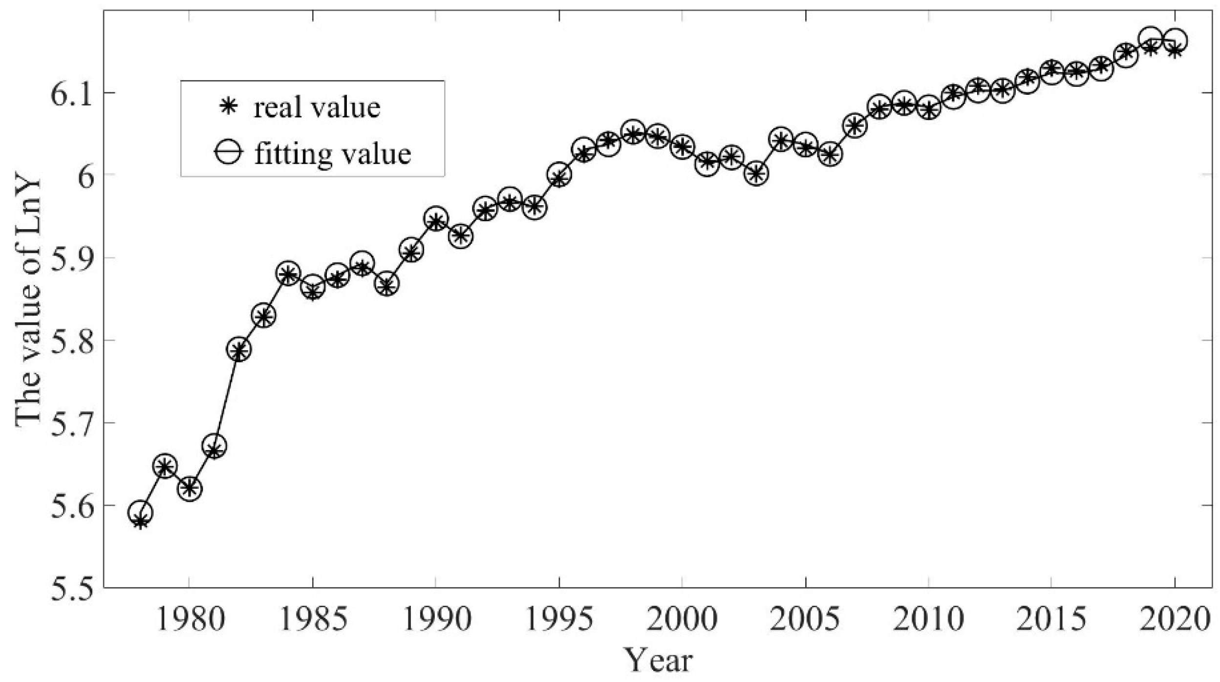
3.1. Data Source

In this study, we will use the national rice production data of China for empirical analysis. The data is extracted from China Statistical Yearbook (1979–2021) and China Agricultural Product Cost-Benefit Compilation (1979–2021).

The data used in this study includes rice yield per unit area $Y_i$(Kg•hm⁻²), material and service cost per unit area of rice $K_i$(CNY•hm⁻²), labor employment per unit area of rice $L_i$(Day•hm⁻²) and annual proportion of crop disasters $Z_i$(%) from 1978 to 2020 in China. The time is year denoted by $t_i,i=1978,\cdots ,2020.$ From the perspective of cost-benefit statistics, rice production costs include material and service costs and labor costs. However, China’s rice production is still based on small-scale decentralized production and management, and it is difficult to accurately measure the labor costs. In China Agricultural Production Cost-Benefit Compilation, the labor costs are mainly composed of the discount of family labor. To avoid double counting the discount of family labor into the model, the material and service cost per unit area and labor employment per unit area in rice represent capital investment and labor input, respectively. The natural disaster is represented by the annual proportion of crop disasters. The value of material and service costs per unit area are adjusted by the price index of means of agricultural production, in which 1977 is the base period.

3.2. Results of Estimation

In the varying-coefficient production function model, the optimal kernel function the Epanechnikov kernel function $H\left(z\right)=0.75{(1-z^2)}_{+}$ is selected. The optimal bandwidths are $h_{1,opt}=0.5383,h_{2,opt}=0.1495,h_{3,opt}=0.1497$, respectively, determined by the cross-validation method. Based on the optimal bandwidths, the annual estimated values of capital elasticity and labor elasticity from 1978 to 2020 are obtained (See Appendix A

Table A1. The values of output elasticity of capital and labor from 1978 to 2020.

Year	α	β
1978	0.3426	−0.1735
1979	0.3504	−0.1757
1980	0.3280	−0.1671
1981	0.3466	−0.1748
1982	0.3497	−0.1756
1983	0.3495	−0.1756
1984	0.3502	−0.1757
1985	0.3408	−0.1728
1986	0.3394	−0.1722
1987	0.3444	−0.1741
1988	0.3382	−0.1717
1989	0.3388	−0.1719
1990	0.3482	−0.1753
1991	0.3337	−0.1697
1992	0.3370	−0.1712
1993	0.3411	−0.1729
1994	0.3246	−0.1656
1995	0.3428	−0.1735
1996	0.3446	−0.1742
1997	0.3302	−0.1681
1998	0.3399	−0.1724
1999	0.3378	−0.1715
2000	0.3209	−0.1640
2001	0.3277	−0.1670
2002	0.3366	−0.1710
2003	0.3239	−0.1653
2004	0.3505	−0.1757
2005	0.3467	−0.1749
2006	0.3399	−0.1724
2007	0.3395	−0.1722
2008	0.3439	−0.1739
2009	0.3455	−0.1745
2010	0.3488	−0.1754
2011	0.3546	−0.1758
2012	0.3555	−0.1757
2013	0.3532	−0.1759
2014	0.3547	−0.1758
2015	0.3550	−0.1758
2016	0.3539	−0.1759
2017	0.3564	−0.1755
2018	0.3566	−0.1755
2019	0.3589	−0.1751
2020	0.3589	−0.1751

). The results show that from 1978 to 2020, the value of capital elasticity is between 0.3209 and 0.3589, with mean 0.3437, and the value of labor elasticity is between −0.1759 and −0.1640, with mean −0.1730.

In this study, the key problem is the estimation of capital elasticity and labor elasticity. To test the reliability of our estimation, we use the same data sets to estimate and compare the capital elasticity and labor elasticity with the varying-coefficient production function model and the C-D production function model, respectively. The data sets are 1978–2016, 1978–2017, 1978–2018, 1978–2019 and 1978–2020, respectively. In the C-D production function model, natural disaster data is missing. The results are shown in

Table 1. Comparison of estimation results of two models.

Data Sets	C-D Production Function Model		Varying-Coefficient Production Function Model
	Capital Elasticity	Labor Elasticity	Average Value of Capital Elasticity	Average Value of Labor Elasticity
1978–2016	0.5046	−0.0518	0.3171	−0.1747
1978–2017	0.5100	−0.0462	0.3315	−0.1738
1978–2018	0.5133	−0.0431	0.3314	−0.1737
1978–2019	0.5159	−0.0406	0.3367	−0.1732
1978–2020	0.5195	−0.0374	0.3437	−0.1730

.

It is observed that the average estimation results of capital elasticity and labor elasticity of the two models are different because of the different construction mechanisms of the models, but the change trends of capital elasticity and labor elasticity are basically the same. Such trends can be explained in other words that, in the past five years, the capital elasticity has an increasing trend, whereas the absolute value of labor elasticity has a slightly decreasing trend. This shows that the application of the varying-coefficient production function model to measure capital elasticity and labor elasticity is worthy of reference. Here, the labor elasticity is negative, indicating that labor input has a negative impact on the growth of rice yield per unit area, and China’s rice production is in the stage of declining marginal return from the labor force.

In fact, using the C-D production function to measure capital elasticity and labor elasticity severely depends on the data set and model variable structure. Different data sets give different elastic estimation. For example, using the C-D production function, Tian et al. [36] obtained that the capital elasticity was 0.1072 and the labor elasticity was −0.0631 based on China’s rice production data from 1991 to 2008. Li et al. [37], based on China’s rice production data from 1978 to 2012, concluded that the capital elasticity was 0.4824 and the labor elasticity was −0.0826. Based on the rice production data of the Sichuan Province from 1980 to 2015, Chen et al. [38] attained that the capital elasticity was 0.2814 and the labor elasticity was −0.0655. As we all know, the C-D production function model is a parametric model, and the varying-coefficient model is a nonparametric model. In statistics, nonparametric models are generally more robust than parametric models. Moreover, using the mean square error (MSE) to evaluate the fitting of the model, we find that based on the rice production data in China from 1978 to 2020, the MSE of the estimation in the varying-coefficient production model is 2.23 × 10⁻⁵, less than the MSE of the estimation in the C-D production function model, which is 1.54 × 10⁻³. To sum up, the use of the varying-coefficient production function model in measuring capital elasticity and labor elasticity depends on the data set, but also the fitting effect and robustness of the model; the varying-coefficient production function model is better than the C-D production function model.

To show the estimated effect, the fitting results of the model are showed in Figure 1, where LnY represents the natural logarithm of Y. The dynamic characteristics of output elasticity of capital and labor are presented visually in Figure 2 and Figure 3, respectively.

In Figure 1, the real values and the fitting values of LnY are shown with asterisks and circles, respectively. The difference between the real values and the fitting values is quite small, thus the estimation of the model is satisfactory. Figure 2 and Figure 3 show that capital elasticity and labor elasticity have obvious fluctuation characteristics in different years. From 1978 to 2004, both capital elasticity and labor elasticity shows an obvious downward trend. From 2005 to 2020, capital elasticity shows an increasing trend, whereas labor elasticity is relatively stable. When the proportion of crop disasters is significantly larger, such as in the years 1980, 1991, 1994, 1997, 2000, 2001 and 2003, the elasticity of capital and labor decrease significantly. It indicates that natural disasters greatly effect rice yield per unit area, as well as the capital elasticity and labor elasticity. As a result, hypothesis (1) in Section 1 is reasonable.

To explore the impact of natural disasters on the output elasticity of capital and labor, scatter plots are drawn with the annual proportion of crop disasters as abscissa and the corresponding elasticity value as ordinate. The results are given in Figure 4 and Figure 5.

It can be seen from Figure 4 that there is a significant negative linear correlation between capital elasticity and annual proportion of crop disasters, with a correlation coefficient of −0.9817. Figure 5 shows that there is also a negative correlation between the absolute value of labor elasticity and annual proportion of crop disasters, with a correlation coefficient of −0.8752. As the annual proportion of crop disasters increases, the decreasing speed of capital elasticity and labor elasticity tends to increase. When the annual proportion of crop disasters is more than about 18%, the elasticity of capital and labor show a significant decline curve. It indicates that capital elasticity and labor elasticity are greatly affected by natural disasters. When natural disasters reach a certain proportion, such as 18%, the capital elasticity and the labor elasticity will decrease rapidly, and at this time, the ability of existing rice production technology to resist natural disasters will decrease rapidly.

3.3. Contribution Rate of Rice Input Factors

To investigate the dynamic characteristics of the contribution rate of input factors to the rice yield growth in China, taking the production level in 1978 as the common comparison object, the contribution rate of each input factor in rice yield growth from 1979 to 2020 are calculated by using the measurement methods described in Section 2.3. The results are shown in Appendix A

Table A2. Input factor contribution rates in rice yield growth from 1979 to 2020.

Year	GTPR/%	NKR/%	KDR/%	TKR/%	NLR/%	LDR/%	TLR/%
1979	42.89	15.06	41.13	56.19	12.77	−11.85	0.92
1980	20.70	40.82	−31.25	9.57	40.75	28.98	69.73
1981	32.38	23.85	16.15	40.00	32.93	−5.31	27.63
1982	58.08	12.68	11.11	23.79	21.20	−3.07	18.13
1983	56.77	17.92	8.97	26.89	18.78	−2.44	16.34
1984	58.71	17.51	7.98	25.49	17.82	−2.01	15.80
1985	58.43	22.51	−2.11	20.41	20.49	0.68	21.17
1986	54.11	28.58	−3.51	25.07	19.68	1.13	20.82
1987	40.66	38.44	1.93	40.37	19.53	−0.56	18.98
1988	32.66	49.63	−5.20	44.43	21.27	1.64	22.91
1989	38.26	46.19	−3.92	42.28	18.25	1.21	19.46
1990	36.56	43.08	5.07	48.14	16.58	−1.28	15.30
1991	41.67	46.05	−8.52	37.53	18.05	2.75	20.80
1992	37.61	48.73	−4.87	43.87	17.04	1.48	18.52
1993	29.94	54.21	−1.28	52.94	16.77	0.36	17.13
1994	34.72	58.95	−15.80	43.15	17.20	4.93	22.13
1995	31.55	52.79	0.17	52.96	15.54	−0.05	15.49
1996	36.37	48.23	1.50	49.73	14.29	−0.39	13.89
1997	46.79	44.78	−8.58	36.20	14.40	2.61	17.01
1998	42.51	43.33	−1.79	41.54	15.48	0.48	15.96
1999	39.60	46.19	−3.33	42.86	16.63	0.90	17.53
2000	52.58	41.04	−15.24	25.80	17.19	4.43	21.62
2001	45.03	44.16	−10.99	33.17	18.68	3.12	21.81
2002	36.06	47.88	−4.43	43.45	19.32	1.16	20.49
2003	41.53	48.63	−14.52	34.11	20.33	4.03	24.36
2004	31.96	43.75	5.46	49.21	19.79	−0.96	18.83
2005	33.58	43.48	2.92	46.40	20.63	−0.61	20.02
2006	31.67	47.98	−1.95	46.03	21.86	0.44	22.30
2007	37.20	43.97	−2.06	41.90	20.44	0.45	20.89
2008	34.68	44.71	0.82	45.53	19.95	−0.16	19.79
2009	33.64	44.58	1.82	46.40	20.30	−0.33	19.96
2010	25.87	49.77	3.98	53.74	21.02	−0.63	20.39
2011	23.07	50.14	7.36	57.50	20.14	−0.71	19.43
2012	18.68	54.07	7.88	61.96	20.01	−0.65	19.36
2013	17.32	56.38	6.53	62.91	20.44	−0.68	19.76
2014	17.52	55.82	7.23	63.05	20.06	−0.62	19.43
2015	17.80	55.86	7.27	63.13	19.65	−0.59	19.06
2016	16.32	57.43	6.71	64.15	20.12	−0.59	19.53
2017	15.74	56.80	8.00	64.80	19.95	−0.48	19.47
2018	18.21	55.02	7.83	62.84	19.38	−0.44	18.94
2019	16.76	55.30	9.04	64.34	19.25	−0.34	18.91
2020	15.30	56.42	9.10	65.52	19.51	−0.33	19.18

. Figure 6 shows the change trend of the contribution rate of the three main production factors to the rice yield growth. The names of the three main contribution rates are total capital contribution rate (abbreviated to TKR), total labor contribution rate (abbreviated to TLR) and generalized technical progress contribution rate (abbreviated to GTPR). We emphasize that this study does not calculate the contribution rate in rice yield growth each year relative to the previous year, because technological progress is a gradual process, and there is little difference in the technical level of rice production between two adjacent years. It is difficult and meaningless to calculate the technological progress of each year, compared with the previous year in rice production.

Figure 6 shows that, compared with 1978, the GTPR of the rice yield growth in China from 1979 to 2020 shows a declining trend in fluctuations, whereas the TKR shows a rising trend in fluctuations and the TLR is relatively stable in the same period. Specifically, from 2000 to 2020, the GTPR decreased significantly. Its value decreased from 52.58% in 2000 to 15.30% in 2020. The value of the TKR increased from 25.80% in 2000 to 65.52% in 2020, an increase of 153.95%. Capital investment became the main factor in rice yield increase. It shows that China’s rice yield growth in recent years has mainly depended on the increase of material and service cost, indicating that it is an extensive and unsustainable growth mode.

3.4. Decomposition of Capital Contribution Rate

It can be seen from Section 3.3 that the increase in rice yield per unit area in China has mainly depended on the increase of capital investment since 2000. To identify which inputs are playing the leading role, this section will decompose the total capital contribution rate for the second time.

In this study, capital investment is measured by the material and service cost per unit area of rice. The material and service cost are composed of seed cost, chemical fertilizer cost, farm fertilizer cost, pesticide cost, agricultural film cost, lease cost (including mechanical operation cost, irrigation and drainage cost, animal power cost, etc.), fuel power cost, technical service cost, tools and materials cost, repair and maintenance cost, other direct costs and indirect costs. We define the weight of each input is the proportion of the cost of each input factor to the material and service cost. The capital contribution rate will be decomposed according to the weight of the input factors. The data is extracted from China Agricultural Product Cost-Benefit Compilation. The results are listed in Appendix A

Table A3. Capital contribution rate and its decomposition from 2000 to 2020.

Year	Seed Cost/%	Chemical Fertilizer Cost/%	Farm Fertilizer Cost/%	Pesticide Cost/%	Agricultural Film Cost/%	Mechanical Operation Cost /%	Irrigation and Drainage Cost/%	Animal Power Cost/%	Fuel Power Cost/%	Other Cost/%
2000	1.98	7.38	0.91	1.93	0.36	2.76	2.33	2.38	0.01	5.77
2001	2.26	9.39	1.17	2.60	0.43	3.64	3.21	2.99	0.00	7.47
2002	3.20	12.00	1.45	3.26	0.54	4.90	3.88	3.51	0.01	10.70
2003	2.48	9.65	1.00	2.87	0.38	4.04	3.16	2.73	0.08	7.71
2004	3.62	15.83	1.79	4.83	0.66	7.11	3.99	3.86	0.21	7.29
2005	3.89	16.29	1.57	5.03	0.70	7.95	3.51	3.26	0.10	4.10
2006	3.93	15.18	1.36	6.06	0.67	9.28	3.57	2.99	0.12	2.88
2007	3.52	13.59	0.99	5.67	0.59	9.40	3.03	2.75	0.07	2.30
2008	3.50	16.54	1.06	5.65	0.56	10.91	2.62	2.56	0.08	2.04
2009	4.10	15.04	1.10	5.66	0.49	12.19	2.81	2.36	0.32	2.34
2010	5.42	15.88	1.34	6.47	0.58	15.72	2.97	2.25	0.22	2.89
2011	5.97	17.44	1.11	6.25	0.58	17.56	3.15	2.09	0.33	3.01
2012	6.60	18.25	1.15	6.69	0.60	20.10	3.04	1.85	0.34	3.33
2013	6.92	17.56	1.10	6.63	0.59	21.46	3.20	1.44	0.39	3.60
2014	7.28	16.22	1.04	6.74	0.60	22.89	2.77	1.36	0.44	3.72
2015	7.30	16.07	1.13	6.75	0.59	23.17	2.73	1.18	0.45	3.77
2016	7.61	15.88	1.13	6.79	0.62	23.93	2.74	0.99	0.51	3.95
2017	7.96	16.04	1.16	6.90	0.59	24.03	2.64	0.75	0.65	4.07
2018	7.74	15.99	1.17	6.54	0.54	23.30	2.53	0.53	0.57	3.93
2019	7.88	16.61	1.14	6.86	0.51	23.73	2.74	0.41	0.65	3.81
2020	8.18	16.47	1.17	7.35	0.51	24.24	2.60	0.32	0.72	3.97

, and the trend for visual perception is shown in Figure 7.

Figure 7 shows that the top four input factors are machinery, fertilizer, seed and pesticide in order of contribution rate. The contribution rate of machinery increases fastest, and machinery becomes the factor with the largest contribution rate among capital investment. The contribution rate of machinery increased from 2.76% in 2000 to 24.24% in 2020. It proves that the mechanization of rice production in China has made great progress. The second most important input factor is chemical fertilizer. The contribution rate of chemical fertilizer increased from 7.38% in 2000 to 18.25% in 2012, and slightly decreased from 17.56% in 2013 to 16.47% in 2020 ranking it second. The third important input factor is seed. The contribution rate of seed increased from 1.98% in 2000 to 8.18% in 2020. The fourth input factor is pesticide. The contribution rate of pesticide increased from 1.93% in 2000 to 7.35% in 2020. Thus, it can be seen that, firstly, since the 21st century, with the rapid growth of agricultural labor costs, machinery plays an increasingly important role in China’s rice production, and the development of rice production mechanization is of great significance to improve the rice yield. Secondly, chemical fertilizer and pesticide play an important role in the rice yield growth, indicating that the current rice production mode in China is not sustainable. In the future, people expect to drastically reduce the use of fertilizers and pesticides in rice production. Finally, the most fundamental way to improve rice yield per unit area is to cultivate good varieties. The application of superior rice varieties has played an increasingly important role in China’s rice yield growth. Based on the improvement of rice varieties and the integration of agro-machinery and agronomy, China’s rice production mode will quickly enter the modernization stage.

4. Discussion

4.1. Policy Implications

The contribution rate of rice input factors is an important basis for the formulation of rice industrial policy. The empirical results presented in this study provide important insights into policy design in the rice industry.

One of the main contributions of this study is to provide a method for measuring the dynamic elasticity and contribution rate of input factors. Using such method, the characteristics of the contribution rate of rice input factors in China from 1979 to 2020 were investigated, and the conclusions from which can be used as a reference for the adjustment of rice industrial policy.

It can be seen from the conclusion in Section 3.2 that, compared with results calculated by our proposed model, the capital elasticity is overestimated, whereas the labor elasticity is underestimated, when using the traditional C-D production function to measure capital elasticity and labor elasticity. As a result, the capital contribution rate is overestimated, the labor contribution rate is underestimated, and the contribution rate of generalized technological progress is distorted. The results in this study show that the contribution of generalized technological progress to China’s rice production presents a downward trend in fluctuations from 1979 to 2012, which is basically consistent with the conclusion by Li et al. (2016) [37]. However, from 2012 to 2020, the downward trend of the contribution rate of generalized technological progress has been significantly alleviated, the labor contribution rate has become more stable, and the capital contribution rate has a slight increasing trend, but the growth rate has slowed down significantly. The results show that since 2012, China’s rice industrial policy has achieved certain success in changing the extensive mode of rice production. In addition, it can be seen from Figure 2 and Figure 3 that the watershed between the dynamic changes of capital elasticity and labor elasticity was 2004. In the same year, the Law of the People’s Republic of China on Promotion of Agricultural Mechanization was promulgated and implemented. Perhaps, such a discovery can be used as one of the bases to test the impact of the Law of the People’s Republic of China on Promotion of Agricultural Mechanization on China’s rice industry.

In the analysis of economic growth, capital is a complex concept. The secondary decomposition of capital contribution rate can measure the contribution rate of various material inputs, thus providing a more targeted basis for the formulation of industrial policies [39]. The results in this study show that, since 2000, although China has made great progress in rice production technology, including the success of super hybrid rice breeding and the gradual maturity of cultivation technology and mechanization technology, the blind expansion of capital investment has reduced the contribution of technological progress to the growth of rice yield per unit area. Among the numerous capital investments in rice production, machinery, chemical fertilizer, seed and pesticide are the four most important input factors. The increase in machinery and seed input at this stage is in line with China’s needs to develop rice mechanization and strengthen variety cultivation. However, the increase of chemical fertilizers and pesticides has restricted the sustainable development of China’s rice industry. With the development and progress of human society, not starving is no longer the only goal of human life, and grain yield is also no longer the only goal of agricultural production. Healthy and delicious food is gradually getting people’s favor. The environmental pollution and food toxicity caused by the residues of chemical fertilizers and pesticides are also being realized and studied [40,41]. In future rice production, we cannot unilaterally pursue the improvement of yield at the cost of environmental pollution and food poisoning. The extensive mode of rice production in China has not been fundamentally changed. Technology and resource constraints remain the “key” issues that perplex the development of China’s rice industry [42]. Strengthening scientific and technological support as well as optimizing the policy system are the inevitable choice for the development of China’s rice industry.

4.2. Advantage of the Proposed Model and Applications in Future Work

Based on the idea of varying-coefficient modeling, the C-D production function is extended to a varying-coefficient production function, which can be used to estimate the dynamic elasticity of input factors and calculate the contribution rate of input factors, providing a new method to study the dynamic characteristics of the contribution rate of input factors in economic growth.

In particular, the analytical ability of the model is expanded due to the introduction of the natural disaster factor. In this model, the contribution rate of an input factor can be decomposed into the net factor contribution rate and the contribution rate of interaction between input factor and natural disaster. For example, it can be seen from Appendix A Table A2 that the natural disaster has a certain impact on the rice yield growth. The value of KDR is between −31.25% and 41.13%, with mean 1.11%. The value of LDR is between −11.85% to 28.98%, with mean 0.61%. The law is concluded as follows: when the annual proportion of crop disaster increases, the KDR is negative, whereas the LDR value is positive and vice versa. This is consistent with intuitive perception. Therefore, when the traditional C-D production function is extended by varying-coefficient production function, the new model can not only be used to measure the dynamic output elasticity and contribution rate of input factors in the study period, but also can be used to explore the interaction between input factors and natural disasters in studying rice yield growth. Such a model can provide a new way for in-depth analysis of the factors in studying economic growth.

Of course, the model can be further improved. When the model is applied, its adaptability needs to be considered. Firstly, in essence, the varying-coefficient production function model belongs to the nonparametric statistical model. To get good results, large samples are generally required. Secondly, the bandwidth has a great influence on the estimation of the coefficient functions. How to determine the optimal bandwidth is still a problem to be further studied [31,32]. Thirdly, the variable, Z, in the elastic functions $\alpha \left(Z\right)$ and $\beta \left(Z\right)$ is not unique. In this study, Z means the annual proportion of crop disasters. In other applications, Z can be represented by other variables such as temperature, concentration, humidity and so on.

5. Conclusions

From the results presented in this study, the following conclusions can be drawn:

(1)

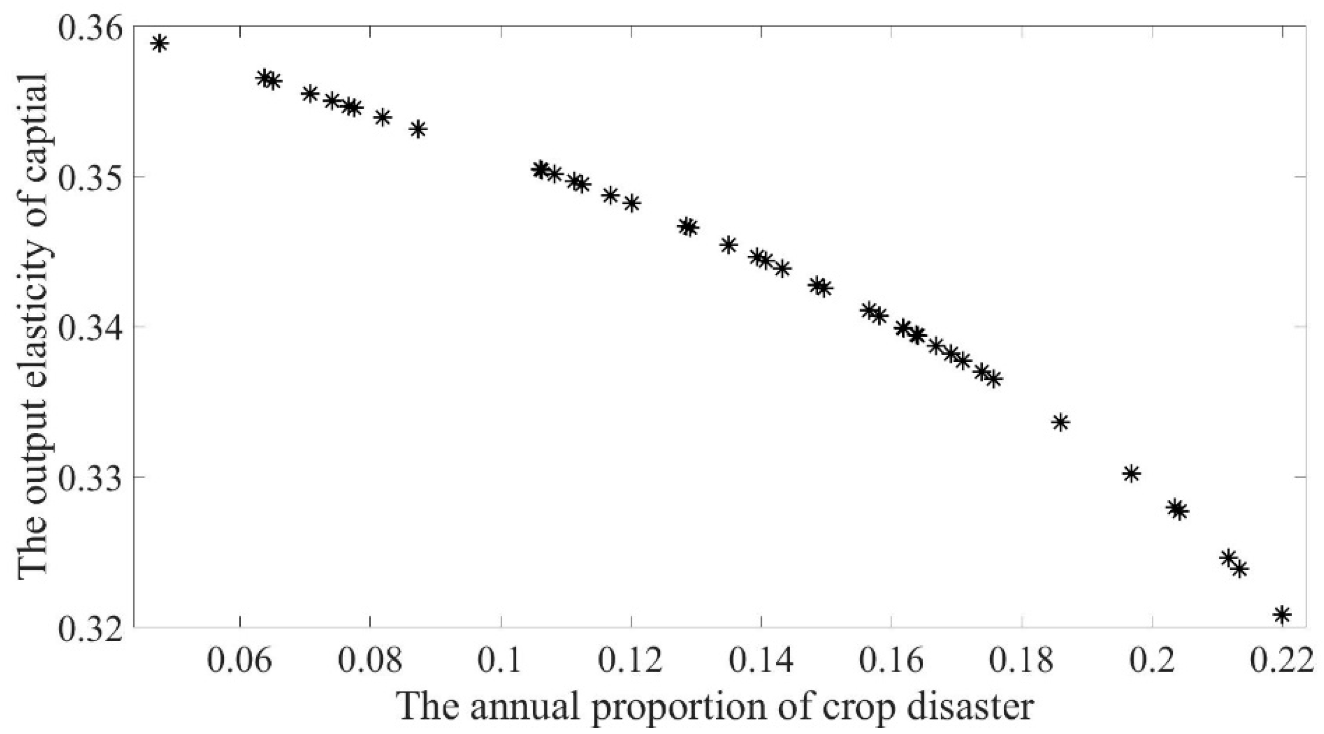
From 1978 to 2020, the value of capital elasticity of rice yield growth in China is between 0.3209 and 0.3589, with mean 0.3437, and the value of labor elasticity is between −0.1759 to −0.1640 with mean −0.1730, indicating capital elasticity and labor elasticity are not constant in different years.

(2)

The correlation coefficient between capital elasticity and the annual proportion of crop disasters is −0.9817, and correlation coefficient between labor elasticity (absolute value) and the annual proportion of crop disasters is −0.8752, presenting a negative relationship for both. With an increase in the annual proportion of crop disasters, the decreasing speed of capital elasticity and labor elasticity tends to increase. When the annual proportion of crop disasters is more than about 18%, the capital elasticity and the labor elasticity show a significant decline curve, proving that natural disasters have a great impact on capital elasticity and labor elasticity. Therefore, we should focus on the long-term strengthening of disaster prevention and resistance. In view of the possibility of the more frequent occurrence of extreme weather events, we should systematically consider various links such as variety cultivation, water conservancy projects, farmland construction, agricultural machinery and agronomy, explore scientific methods, and promote the improvement of the agricultural disaster prevention and relief work system and mechanism.

(3)

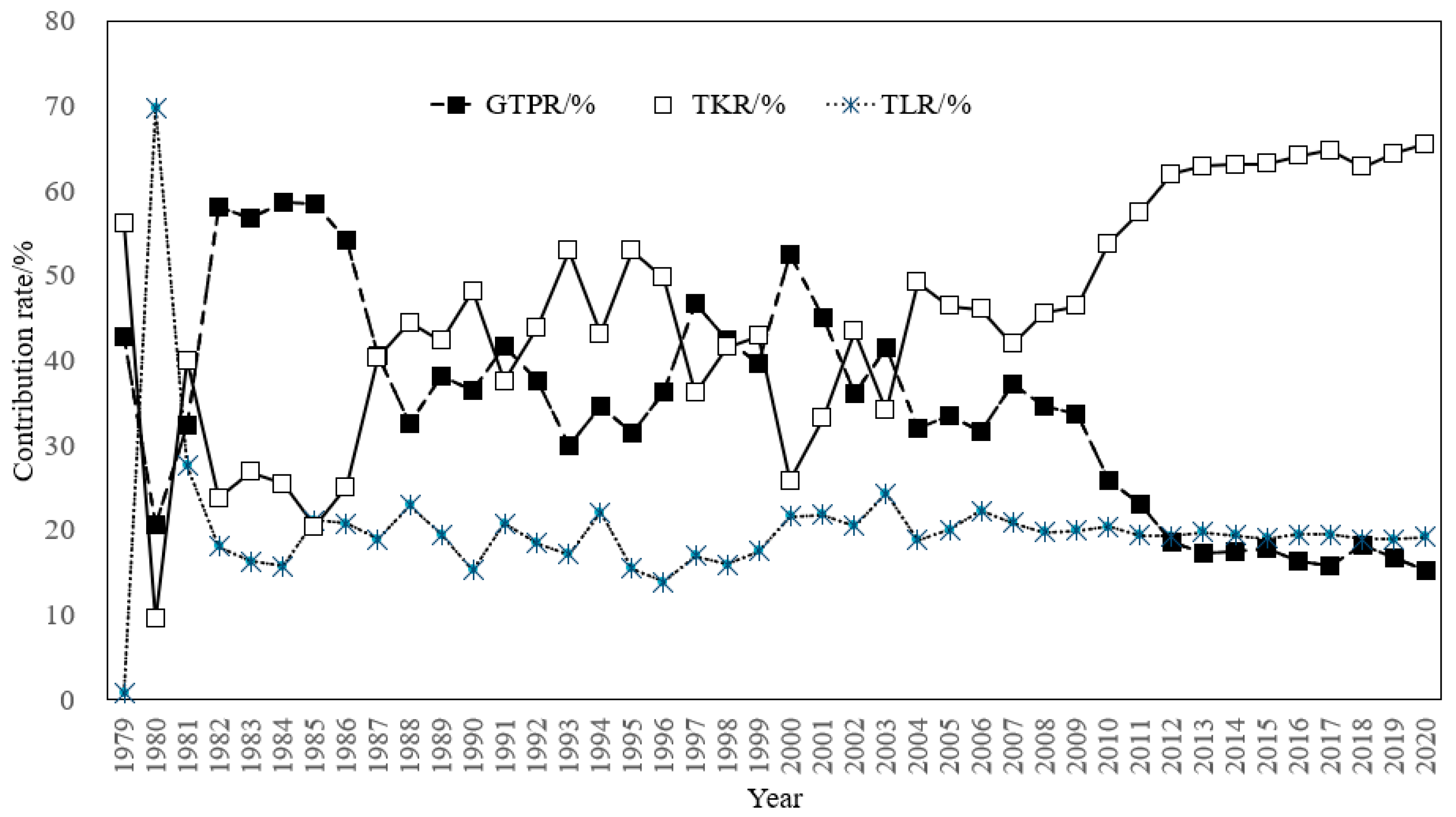
Compared with 1978, the GTPR of China’s rice yield growth from 1979 to 2020 shows a declining trend in fluctuations, whereas the TKR shows a rising trend in fluctuations and the TLR is relatively stable in the same period. The value of GTPR is between 15.30% and 58.71%, the TKR is between 9.57% and 65.52%, and the TLR is between 0.92% and 69.373%. Since 2000, the increase in rice yield per unit area in China mainly depended on the increase of capital investment. The top four input factors are machinery, chemical fertilizer, seed and pesticide in the order of contribution rate. To ensure the sustainable and healthy development of China’s rice industry, it is suggested to reasonably limit the use of chemical fertilizers and pesticides, vigorously develop agricultural mechanization technology, and strengthen rice variety cultivation.

References

1. Mohidem, N.A.; Hashim, N.; Shamsudin, R.; Che Man, H. Rice for food security: Revisiting its production, diversity, rice milling process and nutrient content. Agriculture 2022, 12, 741. [Google Scholar] [CrossRef]
2. FAOSTAT. Production/Yield Quantities of Rice, Paddy in World + (Total) 1978–2020. Food and Agriculture Organization of the United Nations. 2022. Available online: https://www.fao.org/faostat/en/#data/QCL/visualize (accessed on 2 September 2022).
3. Huang, M.; Shan, S.L.; Xie, X.B.; Cao, F.B.; Zou, Y.B. Why high grain yield can be achieved in single seedling machine-transplanted hybrid rice under dense planting conditions? J. Integr. Agric. 2018, 17, 1299–1306. [Google Scholar] [CrossRef]
4. Zhang, X.F.; Wang, D.Y.; Fang, F.P.; Zhen, Y.K.; Liao, X.Y. Food safety and rice production in China. Res. Agric. Mod. 2005, 26, 85–88. [Google Scholar]
5. Ma, G.H.; Yuan, L.P. Hybrid rice achievements, development and prospect in China. J. Integr. Agric. 2015, 14, 197–205. [Google Scholar] [CrossRef]
6. Li, J.J.; Li, J.P. International comparison of rice production cost and benefit and China’s development prospects. China Rice 2021, 27, 22–30. [Google Scholar]
7. Huang, M.; Tang, Q.Y.; Ao, H.J.; Zou, Y.B. Yield potential and stability in super hybrid rice and its production strategies. J. Integr. Agric. 2017, 16, 1009–1017. [Google Scholar] [CrossRef]
8. Xu, L.; Yuan, S.; Man, J.G. Changes in rice yield and yield stability in China during the past six decades. J. Sci. Food Agric. 2020, 100, 3560–3569. [Google Scholar] [CrossRef] [PubMed]
9. Li, Z.H.; Ma, X.; Chen, L.T.; Li, H.W.; Huang, Y.Q.; Li, J.R.; Luo, G.W.; Yao, J.H. Effects of coupling of nursing seedling densities and seedling fetching area on transplanting quality and yield of hybrid rice. Trans. Chin. Soc. Agric. Eng. (Trans. CSAE) 2019, 35, 20–30. [Google Scholar]
10. Espe, M.B.; Hill, J.E.; Leinfelder-Miles, M.; Espino, L.A.; Mutters, R.; Mackill, D.; Kessel, C.V.; Linquist, B.A. Rice yield improvements through plant breeding are offset by inherent yield declines over time. Field Crops Res. 2018, 222, 59–65. [Google Scholar] [CrossRef]
11. Umetsu, C.; Lekprichakul, T.; Chakravorty, U. Efficiency and technical change in the Philippine rice sector: A Malmquist total factor productivity analysis. Am. J. Agric. Econ. 2003, 85, 943–963. [Google Scholar] [CrossRef]
12. Elahi, E.; Cui, W.J.; Zhang, H.M.; Nazeer, M. Agricultural intensification and damages to human health in relation to agrochemicals: Application of artificial intelligence. Land Use Policy 2019, 83, 461–474. [Google Scholar] [CrossRef]
13. Liu, S.W.; Zhang, P.Y.; He, X.L.; Wang, Z.Y.; Tan, J.T. Productivity and efficiency change in China’s grain production during the new farm subsidies years: Evidence from the rice production. Custos E Agronegocio 2015, 11, 106–123. [Google Scholar]
14. Mariano, M.J.; Villano, R.; Fleming, E. Are irrigated farming ecosystems more productive than rainfed farming systems in rice production in the Pilippines? Agric. Ecosyst. Environ. 2010, 139, 603–610. [Google Scholar] [CrossRef]
15. Mariyono, J. Decomposition total factor productivity of Indonesian rice production. Econ. J. Emerg. Mark. 2018, 10, 121–127. [Google Scholar] [CrossRef]
16. Wang, J.Q.; Song, H.H.; Tian, Z.W.; Bei, J.L.; Zhang, H.Y.; Ye, B.; Ni, J. A method for estimating output elasticity of input factors in Cobb-Douglas production function and measuring agricultural technological progress. IEEE Access 2021, 9, 26234–26250. [Google Scholar] [CrossRef]
17. Ball, E.V.; Wang, S.L.; Nehring, R.; Mosheim, R. Productivity and economic growth in U.S. agriculture: A new look. Appl. Econ. Perspect. Policy 2016, 38, 30–49. [Google Scholar] [CrossRef]
18. Li, Z.; Zhang, H.P. Productivity growth in China’s agriculture during 1985–2010. J. Integr. Agric. 2013, 12, 1896–1904. [Google Scholar] [CrossRef]
19. Zhang, S.F.; Xu, B. Production functions with time-varying elasticities and under the catch-up consensus: Total factor productivity. China Econ. Q. 2009, 8, 551–568. [Google Scholar]
20. Solow, R.W. Technical change and the aggregate production function. Rev. Econ. Stat. 1957, 39, 312–320. [Google Scholar] [CrossRef]
21. Shumway, R.H. Applied Statistical Time Series Analysis; Prentice Hall: Englewood Cliffs, NJ, USA, 1988. [Google Scholar]
22. Cleveland, W.S.; Grosse, E.; Shyu, W.M. Local regression models. In Statistical Models in S; Chambers, J.M., Hastie, T.J., Eds.; Wadsworth & Brooks: Pacific Grove, CA, USA, 1991; pp. 309–376. [Google Scholar]
23. Hastie, T.J.; Tibshirani, R.J. Varying-coefficient models. J. R. Stat. Soc. Ser. B 1993, 55, 757–796. [Google Scholar] [CrossRef]
24. Cai, Z.W.; Fan, J.Q.; Li, R.Z. Efficient estimation and inferences for varying-coefficient models. J. Am. Stat. Assoc. 2000, 95, 888–902. [Google Scholar] [CrossRef]
25. Ahmad, I.; Leelahanon, S.; Li, Q. Efficient estimation of a semiparametric partially linear varying coefficient model. Ann. Stat. 2005, 33, 258–283. [Google Scholar] [CrossRef]
26. Luo, X.H.; Yang, Z.H.; Zhou, Y. Nonparametric estimation of the production function with time-varying elasticity coefficients. Syst. Eng. Theory Pract. 2009, 29, 144–149. [Google Scholar]
27. Zhang, S.F.; Xu, B.; Gu, W.T. Statistical and economic tests for the time-varying elasticity production function model. Stat. Res. 2011, 28, 91–96. [Google Scholar]
28. Zhang, S.F.; Zhu, J.N.; Fang, Q.; Liu, Y.X.; Xu, S.W.; Tsai, M.H. Solving the time-varying Cobb-Douglas production function using a varying-coefficient quantile regression model. J. Adv. Comput. Intell. Intell. Inform. 2019, 23, 831–837. [Google Scholar] [CrossRef]
29. Yang, J.; Xiong, W.; Yang, X.G.; Cao, Y.; Feng, L.Z. Geographic variation of rice yield response to past climate change in China. J. Integr. Agric. 2014, 13, 1586–1598. [Google Scholar] [CrossRef]
30. Song, C.X.; Liu, R.F.; Oxley, L.; Ma, H.Y. Do farmers care about climate change? Evidence from five major grain producing areas of China. J. Integr. Agric. 2019, 18, 1402–1414. [Google Scholar] [CrossRef]
31. Zhang, R.Q.; Li, G.Y. Averaged estimation of functional-coefficient regression models with different smoothing variables. Stat. Probab. Lett. 2007, 77, 455–461. [Google Scholar] [CrossRef]
32. Zhang, R.Q.; Feng, J.Y. Varying-coefficient regression models with different smoothing variables. Acta Math. Appl. Sin. 2007, 30, 444–451. [Google Scholar]
33. Fan, G.L.; Xu, H.X. Averaged and integrated estimations of varying-coefficient regression models with dependent observations. Discret. Dyn. Nat. Soc. Hindawi 2019, 2019, 7146793. [Google Scholar] [CrossRef]
34. Lee, Y.K.; Mammen, E.; Park, B.U. Backfitting and smooth backfitting in varying coefficient quantile regression. Econom 2014, 17, 20–38. [Google Scholar] [CrossRef]
35. Yang, S.J. Estimation for semiparametric varying coefficient models with different smoothing variables under random right censoring. J. Korean Stat. Soc. 2018, 47, 161–171. [Google Scholar] [CrossRef]
36. Tian, Y.; Li, B.; Zhang, J.B. Measurement of contribution rate of rice technological progress in China. Stat. Decis. 2012, 350, 93–95. [Google Scholar]
37. Li, Z.H.; Ma, X. Measurement and dynamic characteristics of contribution rate of input factors of rice yield growth in China. Stat. Decis. 2016, 447, 94–97. [Google Scholar]
38. Chen, Y.; Fu, Y.; Zhou, W.; Sun, H.; Wang, T.; Ren, W.J. The change of rice input-output characteristic and influence of technical progress on rice yield in Sichuan province. Chin. J. Agric. Resour. Reg. Plan. 2018, 39, 24–31. [Google Scholar]
39. Wan, Z.; Zhang, C.; Fang, W. Calculation and secondary separation on contribution rate of scientific and technological progress of rice industry in Guangdong province. Technol. Econ. 2012, 31, 63–67. [Google Scholar]
40. Carvalho, F.P. Pesticides, environment, and food safety. Food Energy Secur. 2017, 6, 48–60. [Google Scholar] [CrossRef]
41. Arunrat, N.; Sereenonchai, S.; Chaowiwat, W.; Wang, C.; Hatanno, R. Carbon, nitrogen and water footprints of organic rice and conventional rice over 4 years of cultivation: A case study in the lower North of Thailand. Agronomy 2022, 12, 380. [Google Scholar] [CrossRef]
42. Xu, C.C.; Ji, L.; Li, F.B.; Feng, J.F.; Fang, F.P. Situation and strategies of rice industry development in China. J. Huazhong Agric. Univ. 2022, 41, 21–27. [Google Scholar]
Figure 1. The fitting results of the model.
Agriculture 12 01431 g001
Figure 2. The output elasticity of capital from 1978 to 2020.
Agriculture 12 01431 g002
Figure 3. The output elasticity of labor from 1978 to 2020.
Agriculture 12 01431 g003
Figure 4. The relationship between the output elasticity of capital and the annual proportion of crop disasters.
Agriculture 12 01431 g004
Figure 5. The relationship between the output elasticity of labor and the annual proportion of crop disasters.
Agriculture 12 01431 g005
Figure 6. The contribution rates of rice input factors from 1979 to 2020.
Agriculture 12 01431 g006
Figure 7. The trend of capital contribution rate and its decomposition from 2000 to 2020.
Agriculture 12 01431 g007