Article

Research on Load Spectrum Reconstruction Method of Exhaust System Mounting Bracket of a Hybrid Tractor Based on MOPSO-Wavelet Decomposition Technique

1
School of Automotive and Traffic Engineering, Jiangsu University, Zhenjiang 212013, China
2
State Key Laboratory of Intelligent Agricultural Power Equipment, Luoyang 471039, China
3
First Tractor Co., Ltd., Luoyang 471039, China
*
Author to whom correspondence should be addressed.
Agriculture 2023, 13(10), 1919; https://doi.org/10.3390/agriculture13101919
Submission received: 13 September 2023 / Revised: 28 September 2023 / Accepted: 29 September 2023 / Published: 30 September 2023

Abstract

:
To overcome the limitations of the hybrid tractor bumping tests, which include extended cycle times, high costs, and impracticality for single-part reliability verification, this study focuses on the exhaust system mounting bracket of a hybrid tractor. A novel approach that combines multi-objective particle swarm optimization (MOPSO) and wavelet decomposition algorithms was employed to enhance the reconstruction of shock vibration signals. This approach aims to enable the efficient acquisition of input signals for subsequent shaker table testing. The methodology involves a systematic evaluation of the spectral correlation between the original signal and the reconstructed signal at the stent’s response position, along with signal compression time. These parameters collectively constitute the objective function. The multi-objective particle swarm optimization algorithm is then deployed to explore a range of crucial parameters, including wavelet basic functions, the number of wavelet decomposition layers, and the selection of wavelet components. This exhaustive exploration identifies an optimized signal reconstruction method that accurately represents shock vibration loads. Upon rigorous screening based on our defined objectives, the optimal solution vector was determined, which includes the utilization of the dB10 wavelet basic function, employing a 12-layer wavelet decomposition, and selecting wavelet components a12 and d3~d11. This specific configuration enables the retention of 95% of the damage coefficients while significantly compressing the test time to just 46% of the original signal duration. The implications of our findings are substantial as the reconstructed signal obtained through our optimized approach can be readily applied to shaker excitation. This innovation results in a notable reduction in test cycle time and associated costs, making it particularly valuable for engineering applications, especially in tractor design and testing.

1. Introduction

Hybrid tractors, representing a forefront product in the domain of next-generation tractors, have transitioned from theoretical research and laboratory testing phases towards commercialization. In the initial theoretical research phase, substantial attention was directed toward scheme configuration and energy management strategies [1,2]. However, as the commercialization of hybrid tractors gains momentum, there is a pressing need for increased research emphasis on structural strength, fatigue, and reliability aspects specific to hybrid tractor systems. Reliability assumes paramount significance in the realm of tractor products. The criticality stems from the time-sensitive nature of agricultural production, where any tractor failures that disrupt crop planting or field management operations can result in substantial costs for users. Tractors are used in diverse scenarios, which underscores the necessity for a comprehensive understanding of the intended application contexts, the expected annual usage hours, and the operating practices of the target customers before embarking on durability testing. In contrast to traditional field-based durability testing, there is a growing inclination among researchers and practitioners towards a greater reliance on laboratory testing and simulation within the realm of tractor product development. This shift reflects the industry’s pursuit of innovative approaches to enhance reliability assessment and expedite product development processes [3,4].
The significance of load spectra in vehicle durability engineering is undeniable. However, when it comes to hybrid tractor product development and fatigue failure prediction, their utilization is notably limited. This can be attributed to two primary factors. The first obstacle arises from the diverse nature of tractor operations. Variations in soil conditions and the wide array of supporting implements used result in significant variability in structural load-bearing patterns and load dispersion. This diversity makes it challenging to create a universally applicable load spectrum. Additionally, tractors commonly employ chassis structures crafted from gray iron casting, a material known for its brittleness. The use of gray iron complicates the prediction of fatigue failure. As a result of these challenges, tractor engineering applications frequently rely on the finite element method for static strength calibration [5,6]. This approach entails considering the limit of the conditions of use, thus ensuring that the maximum stress within the structure remains below a certain proportion of the material’s yield strength. While this method is generally conservative, it addresses the complexities associated with load spectra in the context of tractor product development. It is important to note that load profiles previously collected for conventionally powered tractors may not be directly applicable to their hybrid counterparts due to their distinct operational characteristics. Consequently, organizing field and site tests tailored to hybrid tractors becomes a requisite but time-intensive endeavor. Addressing these challenges in the context of hybrid tractors underscores the complexity of and need for comprehensive testing and analysis.
To address the limitations of static strength analysis methods, recent years have seen an increasing focus on tractor load spectrum acquisition and compilation methods. A selection of notable research efforts in this area are summarized below. Mattetti M [7], for instance, monitored the operating parameters of the transmissions of 44 tractors over a year of usage, calculating load amplitudes and frequencies for each transmission component. Pseudo-damages for various failure modes were computed, statistically analyzed, and used to estimate severe damage characteristics. Yan et al. [8] focused on compiling dynamic torque load spectrum for Power Take-Off (PTO) systems under multiple working conditions. They measured PTO torque during typical operations on different soil types, employed the Hilbert–Huang algorithm for signal preprocessing, and utilized rain-flow counting to determine torque amplitude frequency distribution. Changkai Wen [9] introduced a power density-based fatigue load spectrum editing method for accelerated durability testing, tailored to the unique characteristics of agricultural machinery with wide load bandwidths and varying stress amplitudes. This approach employed Short-Time Fourier Transform (STFT) and stress–life curves to derive Accumulated Power Density (AccPD) from load signals, facilitating the extraction of high fatigue damage segments. Wang [10] proposed a method that utilized actual fieldwork data to extrapolate the dynamic load spectrum of the PTO, with a particular focus on the peak-over-threshold model. They developed a mobile tractor PTO loading test bed and a fuzzy proportional-integral-derivative (PID) controller to dynamically apply the PTO load spectrum. Xuedong S et al. [11] collected stress data from the front drive axle of a four-wheel-drive tractor and used the rain-flow counting method to prepare the strain load spectrum of the front axle. Their novel parameter identification method employed a genetic algorithm (GA) for efficient parameter search. Yang [12] introduced a load spectrum extrapolation method with optimal threshold selection based on genetic algorithms. This method utilized pin force sensors to measure ploughing resistance in tractor three-point suspension devices and employed the generalized Pareto distribution (GPD) to fit extreme load distributions for extrapolation. Collectively, these studies represent the diverse range of approaches to tractor load spectrum acquisition and compilation and offer valuable insights into improving the accuracy of fatigue failure prediction in agricultural machinery.
In response to the challenge of high load dispersion, numerous scholars have undertaken load spectrum collection efforts, aiming to encompass a broader range of soil types and operational scenarios. However, they often find themselves limited to the predominant local operation types. China, with its diverse regional agronomic requirements, underscores the complexities of this issue. The multitude of ways in which tractors are employed further underscores the reliance on durability evaluation through test methods, as field tests are inherently seasonal and rarely align with enterprise product development schedules. As an illustration of global practices, H.W. [13] and colleagues conducted load spectrum testing for modern agricultural implements at the German Agricultural Machinery Society’s (DLG) bump test site. They integrated the rain-flow cycle counting algorithm with Miner’s linear damage rule to assess cumulative fatigue damage. Notably, their test design achieved a substantial time acceleration factor of 3.5 compared to field tests, demonstrating the utility of such approaches in tractor reliability verification.
This paper focuses on the shock vibration test data analysis of the exhaust system mounting bracket in a tandem hybrid tractor. Traditionally, tractor bump tests are employed to evaluate the fatigue durability of multiple components within the entire vehicle. However, these tests can be both costly and time consuming. Therefore, durability verification, particularly for critical components such as the exhaust system, is often conducted through alternative means, such as shaker testing or simulation. In this paper, the load time history data from the exhaust system mounting bracket during the tractor bump test were collected. Then a novel approach, combining multi-objective particle swarm optimization and wavelet decomposition was introduced, to reconstruct the shock vibration load spectrum for tractor durability testing. The primary objective is to retain the essential characteristics of the vibration shock load spectrum while significantly reducing the signal time’s duration. This involves careful selection of the wavelet decomposition function type and the number of decomposition layers. The newly proposed methodology achieves a remarkable reduction in load spectrum time while retaining over 90% of the original load’s damage characteristics. This reduction contributes significantly to reducing shaker test time and associated costs.

2. Materials and Methods

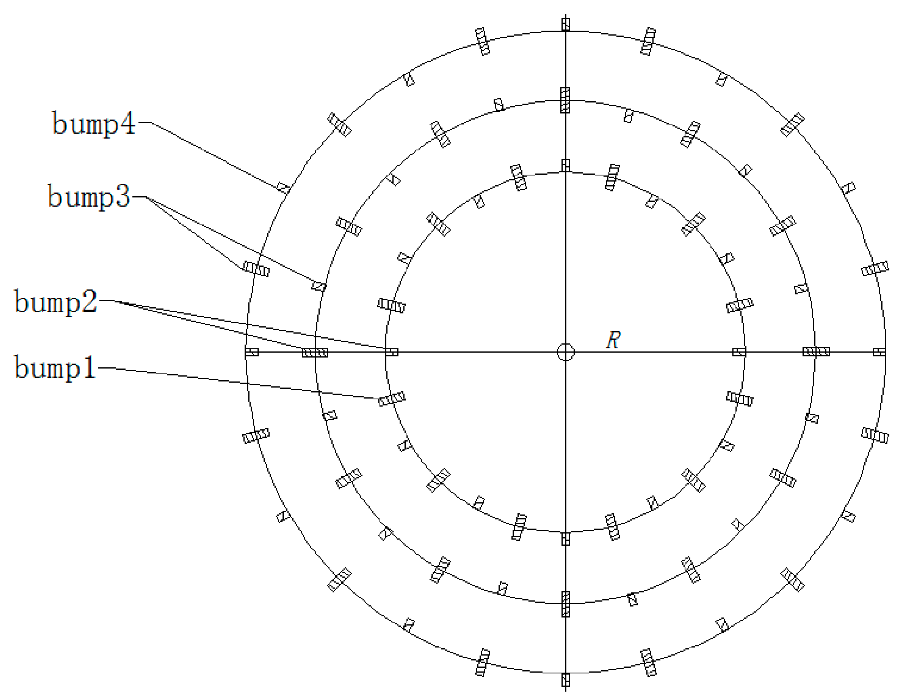
2.1. Shock Vibration Load Spectrum Acquisition

According to the Chinese national standard GB/T 3871.20-2015, titled ‘Agricultural Tractor Test Procedures Part 20: Bump Test’ [14], obstacles of different specifications are distributed on the circular test site, and their configurations are depicted in Figure 1. These obstacles serve a specific purpose within the test scenario. When a tractor navigates through a double row of obstacles all of its wheels experience simultaneous impacts. Conversely, when it passes through a single row of obstacles, only wheels on one are impacted. Within the predefined fixed radius of the test site, there are precisely 12 double-row obstacles and 12 single-row obstacles. It is noteworthy that the spacing between these obstacles must exceed 1.5 times the wheelbase of the wheeled tractor being tested.
During the test, adjustments were made to the tire pressure and vehicle speed to achieve specific vertical vibration acceleration levels. The target values were set at 40 m/s2 for the front axle and 25 m/s2 for the rear axle of the tractor. In accordance with the testing protocol, wheeled tractors with an engine power exceeding 36 kW were subjected to a rigorous testing regimen. This involved subjecting the tractor to a specified number of bumps, which, as per the protocol, was set at 80,000 bumps.
The main parameters of the test tractor in this paper are shown in Table 1.
Figure 2a depicts the test scene in alignment with the bump test conditions described previously. Vibration tests were executed by strategically placing vibration sensors at two crucial locations: the center of the tractor’s front axle and the center of the rear axle. These sensors were instrumental in determining the appropriate driving speed. In this study the vehicle traveled at a consistent speed of 7 km/h during the test, and the engine’s primary operational speed was in the range of 1600 r/min. Vibration acceleration sensors were strategically positioned at three key measurement points: the bracket mounting position (Measurement Point 1), the midpoint of the bracket (Measurement Point 2), and the base of the exhaust system (Measurement Point 3). The precise locations of these three measurement points are illustrated in Figure 2b. Data acquisition was facilitated using a B&K LAN-XI module, which operated at a sampling frequency of 25 kHz. A high pass filter was applied, set at 0.7 Hz, to ensure accurate data sampling.

2.2. Signal Reconstruction Based on MOPSO-Wavelet Decomposition Technique

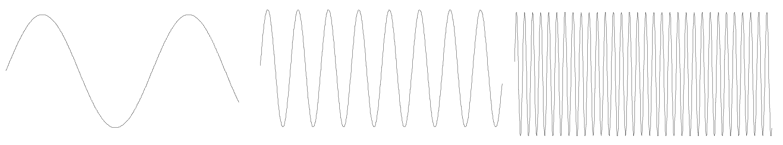
2.2.1. Wavelet Decomposition

The Fourier transform holds a pivotal position in signal processing methods as it effectively bridges the time and frequency domains. However, it is not without limitations. The Fourier transform provides an overall transformation but fails to capture the time-varying characteristics of a signal, making it less suitable for processing non-stationary signals. To address this limitation, the Short-Time Fourier Transform (STFT) was developed. It views unsteady signals as a superposition of a series of short-time smooth signals by applying a time window. Abdullah S. et al. [15] and Panu P. et al. [16] pioneered the use of STFT in studying part loads. However, STFT has its limitations, for example, obtaining a high-frequency resolution requires the use of a long time window. This poses a challenge since time localization and frequency localization are often contradictory, particularly for signals with high frequencies, such as shock vibrations. By contrast, the wavelet transform employs a variable time window to finely capture the local features of a signal. As shown in Figure 3 and Figure 4, unlike the Fourier transform, which uses trigonometric functions as basic functions, the wavelet transform employs wavelet functions as basic functions. These wavelet functions have the advantage of better portraying the local characteristics of the signal [17].
One widely utilized approach is the Empirical Mode Decomposition (EMD) algorithm, which is particularly effective in extracting fault signals exhibiting amplitude modulation (AM) or frequency modulation (FM) characteristics. EMD operates adaptively by decomposing signals based on their inherent characteristics. However, it is noteworthy that EMD lacks rigorous mathematical theory support and its decomposition process primarily relies on empirical knowledge. The low-frequency IMF component is susceptible to cumulative leakage rendering it effectively impractical or less informative in certain applications. In this study, we analyzed the intrinsic frequency characteristics of the system, as presented in Table 5. Within the low-frequency range spanning tens of hertz to tens of hertz, the influence of this component cannot be overlooked. To draw a conclusive comparison, we have conducted a comparative analysis with other algorithms and the results clearly demonstrate the superior performance of the wavelet decomposition algorithm.
The application of the wavelet transform in load spectrum editing encompasses two primary aspects. First, it serves as a tool for noise reduction and for the removal of trend terms, anomalies, and other unwanted elements from the test signal [18,19]. Secondly, the wavelet transform plays a crucial role in reconstructing the original signal to derive the accelerated load spectrum [20,21,22]. In reference [22], the authors applied the wavelet decomposition technique to transform the measured tractor power take-off (PTO) torque signal into a stress-time signal. Subsequently, they utilized this technique to obtain a reduced accelerated load spectrum, aiming to validate the effectiveness of the accelerated time load spectrum with respect to pseudo-damage retention. However, it is worth noting that similar methods often do not delve deeply into the intricacies of the wavelet decomposition process. The choices made regarding the type of wavelet basic function, the number of decomposition layers, and the selection of specific wavelet components significantly impacted the final results in load spectrum reprogramming.
The prevailing wavelet decomposition method in current use is the Mallat algorithm. This algorithm initiates the decomposition process by splitting the initial signal into two fundamental components: the ‘low-frequency approximation’ (a1) and the ‘high-frequency details’ (d1). Subsequently, the same decomposition operation is iteratively applied to the ‘low-frequency approximation’ part from the previous step, resulting in a further subdivision into ‘low-frequency approximation’ and ‘high-frequency details.’ This recursive subdivision process continues until the desired level of decomposition or detail is achieved.
The Mallat algorithm relies on wavelet filters, denoted as h0 and h1, for signal decomposition and filters g0 and g1 for coefficient reconstruction. The decomposition process is as follows:
{ a 0 ( n ) = f ( n ) a j ( n ) = k h 0 ( k 2 n ) a j 1 ( k ) d j ( n ) = k h 1 ( k 2 n ) a j 1 ( k )
where j is the number of wavelet decomposition layers, h0 is the low-pass decomposition filter, and h1 is the high-pass decomposition filter. The algorithm assumes that a0(n) is equal to the discrete signal f(n), and that the wavelet coefficients aj of the approximate part of f(n) on layer j are obtained by convolving the wavelet coefficients of the approximate part of the wavelet coefficients aj−1 on layer j−1 with h0 and then sampling the operation at intervals. The detail part dj of the signal f(n) on layer j is obtained by convolving the wavelet coefficients aj−1 of the proximate part of layer j−1 with h1 and then sampling at intervals. By using the decomposition shown in Equation (3), the wavelet coefficients aj−1 of the approximate part of layer j−1 are decomposed into two parts: wavelet coefficients aj of the approximate part of layer j and wavelet coefficients dj of the detailed part of layer j. The wavelet coefficients dj−1 of the detailed part of layer j−1 do not continue to be decomposed in layer j. At layer j, the discrete sequence f(n) is finally divided into aj, dj, dj−1, ......, d2 and d1. The wavelet decomposition process is shown in Figure 5.
The wavelet reconstruction algorithm is defined as:
a j ( n ) = k g 0 ( n 2 k ) a j + 1 ( k ) + k g 1 ( n 2 k ) d j + 1 ( k )
where g0 is a low-pass reconfiguration filter and g1 is a high-pass reconfiguration filter. The wavelet coefficients aj of the approximated part of the signal f(n) in the (j)th layer are composed of two parts. The first part is the wavelet coefficients aj+1 of the approximated part of the (j+1)th layer after interpolating the zeros at the intervals and convolving them with g0. The second part is obtained by interpolating the zeros of the wavelet coefficients of the detail part of the (j+1)th layer dj+1 intervals and then convolving them with g1. Repeat this process until layer 0 to get the completely reconstructed signal. The wavelet reconstruction process is shown in Figure 6.

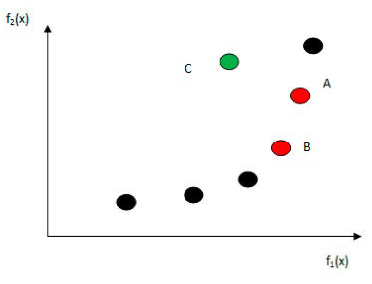
2.2.2. Multi-Objective Particle Swarm Optimization

A diverse array of basic functions for wavelet packet decomposition exist and each possess distinct properties that can capture various characteristics of a signal. The selection of specific wavelet decomposition parameters is contingent upon the optimization of achieving predefined goals. The field of optimization problems has yielded numerous outstanding results throughout human development, and with the advancement of computer-solving capabilities, numerical methods have gained prominence. One notable category of optimization algorithms is swarm intelligence algorithms (SI) [23], which emulate various social group behaviors exhibited by animals to address large-scale, nonlinear optimization problems. Currently, prominent examples of swarm intelligence algorithms include the particle swarm algorithm, ant colony algorithm, gray wolf algorithm, whale algorithm, and others [24,25,26]. It is essential to recognize that population intelligence optimization algorithms, including those mentioned, are susceptible to the premature convergence problem, in which they may converge to a local optimum prematurely. Conversely, the particle swarm optimization algorithm boasts numerous successful cases of addressing this issue through various enhancements. Consequently, we have opted for the particle swarm optimization algorithm in this paper. The particle swarm optimization algorithm harnesses the collaborative potential among individual particles within a group to address finite-space optimization problems. In the optimization process, each particle leverages its own historical knowledge and exchanges information with the group to dynamically adapt its flight speed and direction. This collaborative behavior allows the swarm to effectively explore and exploit the search space for optimal solutions.
With the objective of minimizing the function F(X), the optimal position for particle i can be ascertained using the following equation:
P i ( t + 1 ) = { P i ( t ) , F ( W i ( t + 1 ) ) F ( P i ( t ) ) W i ( t + 1 ) , F ( W i ( t + 1 ) ) < F ( P i ( t ) )
where Pi represents the best position previously encountered by particle i, and Wi denotes the current position of particle i.
The position denoted as Pg(t), referred to as the global best position, is the collective optimal position achieved by all particles in the population. Consequently, we can state the following:
P g ( t ) { P 0 ( t ) , P 1 ( t ) , , P x ( t ) } | F ( P g ( t ) ) = min { F ( P 0 ( t ) ) , F ( P 1 ( t ) ) , , F ( P x ( t ) ) }
By defining Vi as the current velocity of particle i, we can formulate the evolution equation for the fundamental particle population as follows:
v i j ( t + 1 ) = v i j ( t ) + c 1 r 1 j ( t ) [ p i j ( t ) w i j ( t ) ] + c 2 r 2 j ( t ) [ p g j ( t ) w i j ( t ) ]
w i j ( t + 1 ) = w i j ( t ) + v i j ( t + 1 )
where j represents the jth dimension of the particle, i refers to the particle index, t stands for iterations, c1 and c2 are acceleration constants, and r1 and r2 are random numbers uniformly distributed in the range (0, 1).
Population-based intelligence optimization algorithms often encounter issues such as falling into local optima and poor convergence. To address these challenges and enhance the ability of particles to perform global exploration in the early stages and local exploitation in the later stages, it is common practice to adjust the weighting of the current velocity. This adjustment can be expressed as a modification of Equation (6):
V i ( t + 1 ) = ω V i ( t ) + c 1 r 1 ( t ) [ P i ( t ) W i ( t ) ] + c 2 r 2 ( t ) [ P g ( t ) W i ( t ) ]
ω ( t ) = M 1 t N max × M 2
where Nmax represents the maximum number of iterations, and the inertia weights are treated as a function of the t. Specifically, these weights progressively decrease from M1 to M2 as the number of iterations increases.
Many practical optimization problems involve multiple objectives. When tackling a multi-objective optimization problem using a particle swarm algorithm, it is crucial to establish clear definitions for local and global optimal solutions as these definitions guide the evolutionary trajectory of the population. Multi-objective optimization tasks require a comprehensive consideration of the degree to which each objective is achieved; however, the focus is not solely on optimizing a single objective but rather on striking a balance among multiple objectives. The multi-objective particle swarm optimization (MOPSO) algorithm, originally introduced by Coelle in 2002, has undergone significant refinement and development by numerous scholars. It has found extensive applications in various engineering domains [23,24].
This paper addresses the reconstruction of the shock vibration load spectrum of a tractor, with two primary objectives. First, the reconstructed signal aims to preserve the structural damage characteristics to the maximum extent. Second, it strives for signal compression to minimize bench vibration test duration. Thus, the multi-objective standard optimization function in this study is defined as follows:
F ( x ) = { max f 1 ( x ) min f 2 ( x )
where f1(x) represents the shock vibration damage retention coefficient, and f2(x) denotes the signal time compression ratio. It is evident that these two objectives are inherently contradictory.
The decision vector, denoted as ‘x = (x1,x2,…xD)’, is of dimension D. In this paper, D is set to 48, indicating that each particle consists of 48 dimensions. Among these dimensions, 26 pertain to the wavelet basic functions, 10 correspond to the number of seed decomposition layers, and the remaining 13 dimensions relate to the wavelet components utilized for signal reconstruction.
The 26 wavelet basic functions are Haar, db3, db4, db5, db6, db7, db8, db9, db10, Meyer, Dmeyer, Gaussian, MexicanHat, Morlet, sym2, sym3, sym4, sym5, sym6, sym7, sym8, coif1, coif2, coif3, coif4, and coif5, which encompasses the most commonly used options.
The number of decomposition levels, which varies between 3 and 12, is represented by 10 dimensions within the decision vector. For the majority of signals, increasing the number of layers beyond a certain threshold, typically exceeding 10 layers, does not significantly enhance the signal decomposition process. In light of this observation, this paper opts for a pragmatic approach by selecting 12 layers for decomposition [27].
Within the 12-layer wavelet decomposition, there can be as many as 13 components, hence the allocation of 13 dimensions to represent the wavelet components.
In the process of solving multi-objective optimization problems, a critical aspect lies in the storage and continuous update of the non-dominated solution set. The concept of non-dominated solutions draws its theoretical foundation from Pareto dominance relations. As exemplified in Figure 7 where A, B, and C denote the objective function values corresponding to three solution vectors, namely x1, x2, x3, within the objective space. Notably, C represents the smallest value of f1(x) and the largest value of f2(x). Consequently, solution vector x3 is dominated by both x1 and x2. However, it remains impossible to definitively establish whether A or B is superior. Consequently, no dominance relationship exists between x1 and x2, rendering them all non-dominated solutions. The essence of solving a multi-objective optimization problem lies in the quest to identify and characterize all non-dominated solutions.
In this paper, the optimization of wavelet parameters for reconstructing tractor impact vibration load spectra is carried out using a multi-objective particle swarm algorithm. The methodology is detailed as follows:
  • To begin, define the population size and the dimensions of each particle. Then initialize both the position and velocity of every particle within the population.
  • Calculate the fitness of each particle by evaluating the objective functions f1(x) and f2(x) for every particle.
  • Store the non-dominated solution in external memory.
  • Update the individual optimum and the global optimum and update the position and velocity of each particle.
As the number of iterations increases, the average velocity of all population particles gradually diminishes, signifying the convergence of the population. To mitigate premature convergence into local optima, this paper employs a strategy of selecting a particle that lies further from the others among the top 10 particles based on congestion distance ranking as the global optimal particle. This approach is adopted to preserve solution diversity.
5.
Recalculate the value of the objective function for each particle.
6.
Non-dominated solution sets update.
In this paper, the maximum capacity of the external memory is defined as 30. The Crowding Distance algorithm is employed for updating the external memory. The crowding distance of each particle is defined as follows:
L ( x j ) = i = 1 N ( f i ( x j + 1 ) f i ( x j 1 ) f i max f i min ) , N = 2
where L(xj) represents the crowding distance of the jth particle, and N is the number of objective functions, and fi denotes the ith objective function. Additionally, f i max and f i min correspond to the maximum and minimum values of the ith objective function, respectively. Furthermore, fi(xj+1) and fi(xj−1) refer to the values of the two individuals closest to particle j along the ith objective function.
The particles are sorted in descending order based on their crowding distance, and subsequently, the particle with the smallest crowding distance is systematically removed from the external memory.
7.
Increment the optimization counter by 1 and assess whether the number of iterations is adequate. If it is deemed insufficient, return to step 4 for further optimization. Otherwise, conclude the iteration process and output the non-dominated solution set stored in the external memory.
To visualize the flow of the algorithm better it is shown in Figure 8.

3. Results and Discussion

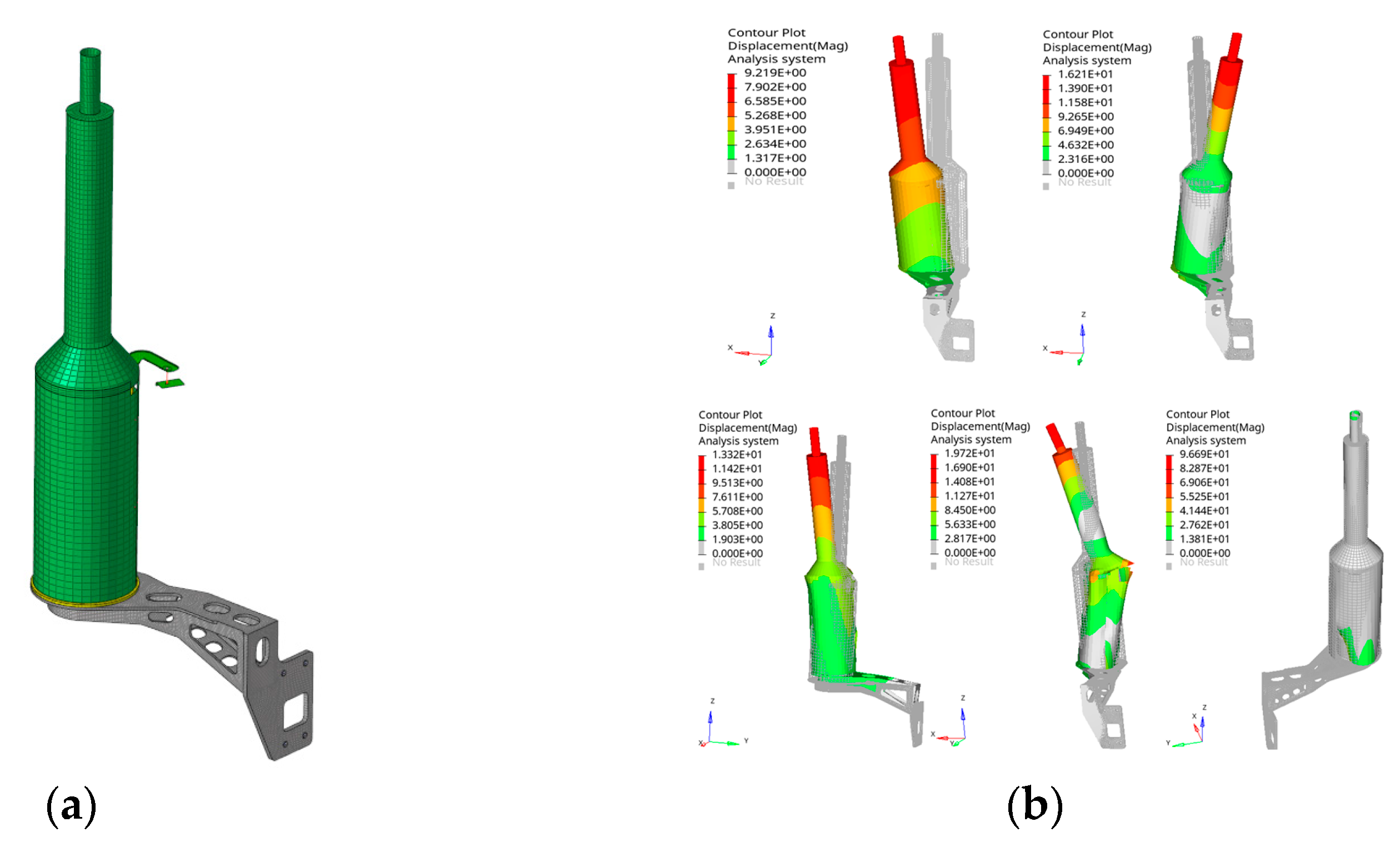
3.1. Modal Analysis of Exhaust System Mounting Bracket

Modal analysis serves as the most intuitive method for understanding the system characteristics and the foundation of dynamics analysis methods. It is employed to extract crucial information such as modal frequencies and vibration modes, which subsequently facilitate the analysis of acquired signals in practical applications. Additionally, as previously mentioned, engineering applications often involve the calibration of tractor structural components’ reliability through static strength analysis [28,29]. Nevertheless, this analysis method necessitates a prerequisite: the intrinsic frequency of the structure must significantly surpass the excitation frequency. Hence, conducting a modal analysis of the exhaust system and its mounting bracket becomes imperative to ascertain the intrinsic frequencies at each order.
The typical configuration involves the rigid bolting of the exhaust system mounting bracket to the engine flywheel housing. The bracket is constructed from Q235 material, and its material properties are detailed in Table 2.
Utilizing the finite element analysis software Hyper-Works, the finite element model was constructed, as depicted in Figure 9a. Subsequently, we computed the first five modes of modal vibration for the system, as depicted in Figure 9b. The corresponding intrinsic frequencies are detailed in Table 3.
The tractor under study features an inline six-cylinder four-stroke diesel engine, with an idle speed of 750 r/min. Using Equation (12), the ignition frequency at idle is calculated to be 37.5 Hz. Remarkably, this ignition frequency aligns closely with the third-order intrinsic frequency of the exhaust system, posing a resonance risk. Similarly, calculations reveal that the fourth-order intrinsic frequency of 79.0 Hz corresponds to an engine operating speed of 1580 r/min, while the fifth-order intrinsic frequency of 79.0 Hz corresponds to an engine operating speed of 2114 r/min. Consequently, these intrinsic frequencies exhibit resonance tendencies at specific engine speeds, rendering traditional static strength analysis inadequate for assessing the reliability of this bracket.
f = 2 n z 60 τ
where n indicates the speed of the engine, z indicates the number of cylinders of the engine, and τ indicates the number of strokes of the engine.

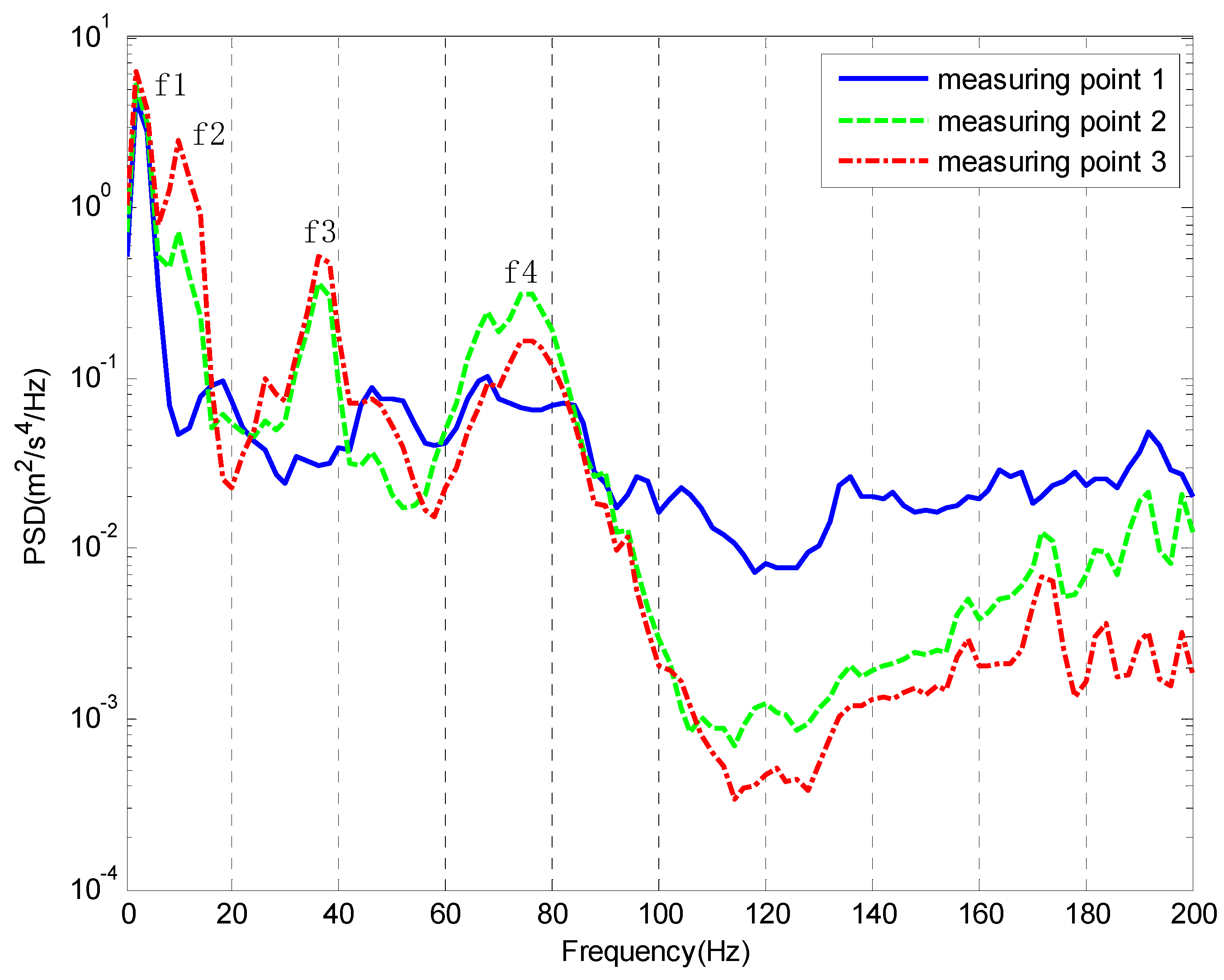
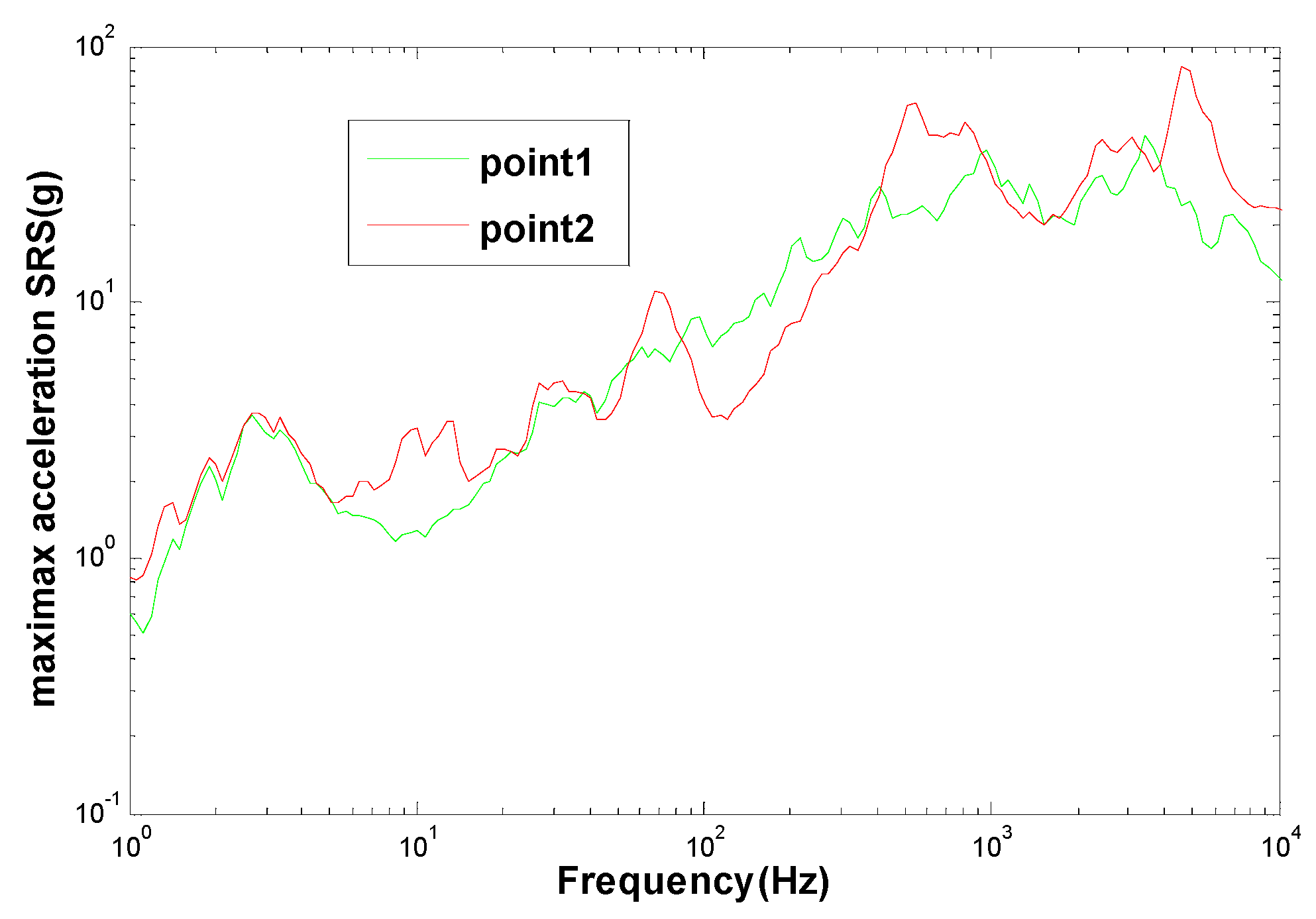
3.2. Time-Frequency Domain Analysis of Test Signals

A three-axis acceleration vibration sensor was employed for the test, where the X direction corresponds to the forward direction of the vehicle, the Y direction represents the lateral direction, and the Z direction signifies the vertical direction. During the test, the tractor traversed the field for approximately 50 s. The resulting time-domain vibration curves in the three directions at measurement point 1 are depicted in Figure 10. Furthermore, Table 4 provides an overview of the time-domain statistical characteristics of the vibration signals recorded in the X, Y, and Z directions at all three measurement points.
Measurement point 1, positioned at the bracket mounting location, serves to characterize the magnitude of the excitation transmitted to the bracket. In contrast, measurement points 2 and 3, situated at the middle and end of the bracket, respectively, capture the response under excitation. The power spectral density curves of the Z-direction vibration signals at these three measurement points are presented in Figure 11. Notably, the power spectral density curves of measurement points 2 and 3 exhibit remarkable similarity, owing to their shared location within the same vibration system and closely aligned frequency response characteristics. The series of peak frequencies observed in the curves in Figure 11 can be attributed to either the frequency of the excitation signal or the intrinsic frequency of the system. Notably, a peak exists at all ‘f1’ positions, which we attribute to the vehicle’s overall intrinsic frequency. The intrinsic frequency of the entire tractor is influenced by factors such as tire properties and vehicle weight and typically falls within the range of 3 to 5 Hz. Furthermore, the power spectral density curves of measurement points 2 and 3 display consistent peak distributions at positions denoted as ‘f2’, ‘f3’, and ‘f4’. These peaks can be reliably associated with the first-, third-, and fourth-order intrinsic frequencies of the post-processing system, a conclusion which is supported by the modal analysis results presented in Table 2. The peak frequencies are tabulated in Table 5, and the curves serve to corroborate the accuracy of the finite element modal analysis results.

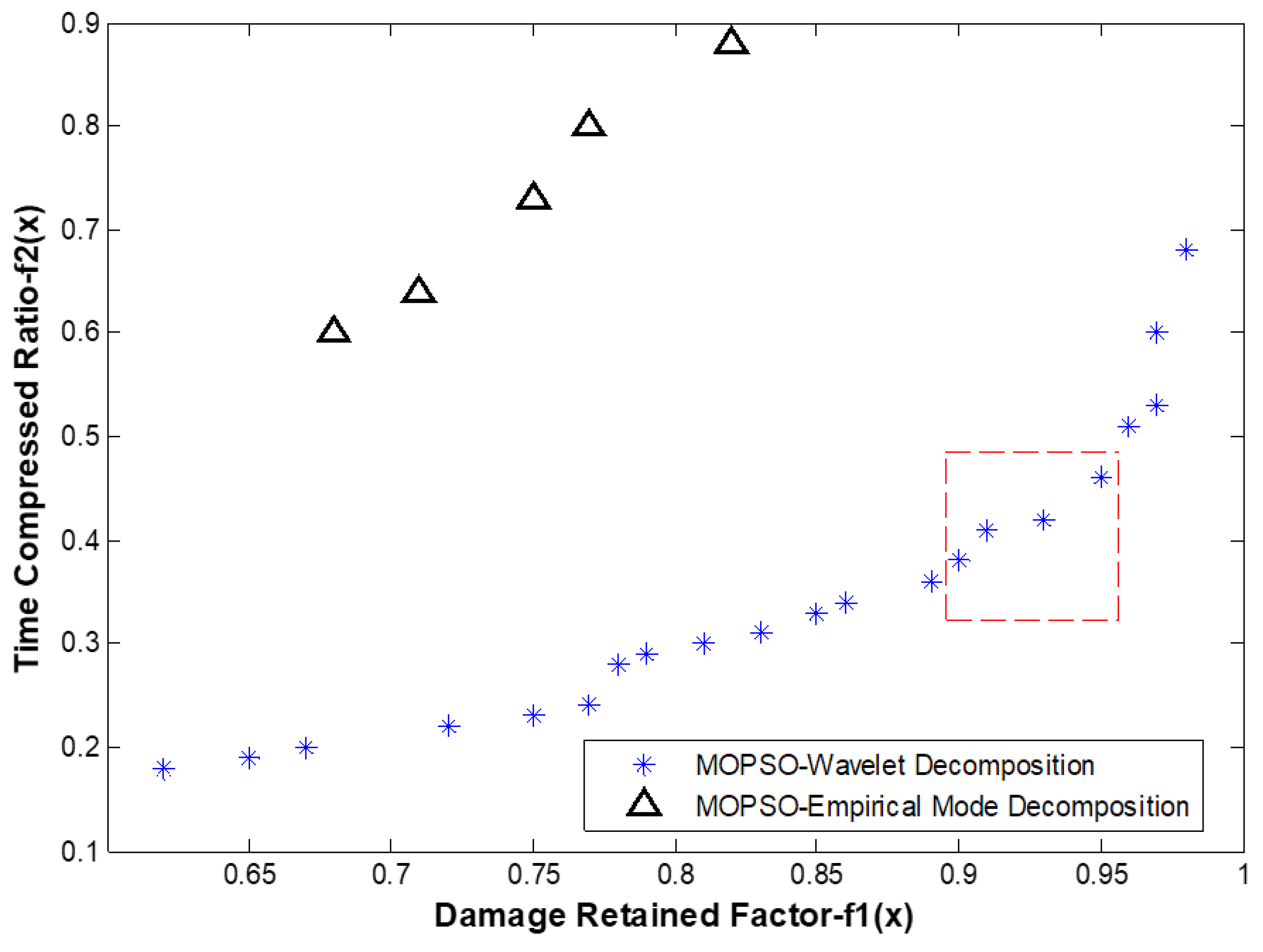
3.3. Wavelet Decomposition and Reconstruction of Test Signals

In conventional studies on load spectrum editing methods, the principle of fatigue damage equivalence is often employed, typically aiming to retain more than 90% of the original damage. To estimate the fatigue damage experienced by a structure, stress or strain signals are experimentally collected, load cycles are extracted using methods such as the rain-flow counting method, and the accumulated fatigue damage is calculated based on the Miner criterion and the S–N curve specific to the component. While this approach yields the actual damage experienced by the component, practical engineering applications more commonly involve generalized loads, such as acceleration, displacement, and force, which are easier to measure. In such cases, the pseudo-damage concept is employed. It involves utilizing specified standard S–N curves and applying the same damage accumulation methodology to compute a damage value, often referred to as pseudo-damage. Pseudo-damage calculations are straightforward and do not necessitate detailed structural knowledge, a factor which has led to their widespread adoption in the durability testing of vehicles and components [30]. However, the primary drawback of the pseudo-damage calculation method lies in its failure to consider the unique characteristics of the structure itself. Consequently, it cannot capture the distinctions between loads acting on structures with differing inherent frequencies. Hence, in this study, we opted to evaluate the validity of the reconstructed signals by assessing the correlation of impact response spectra at the brace response points.
Analyzing the Power Spectral Density (PSD) curves presented in Figure 11 reveals a notable disparity between the spectrum of measurement point 1 and that of measurement points 2 and 3. If we treat the bracket and exhaust system as a linear time-invariant system, we can consider the vibration signal at measurement point 1 to be the input to the system, and the vibration signals at measurement points 2 and 3 as the system’s responses. We can establish the response relationship between them as follows:
X ( ω ) = H ( ω ) F ( ω )
where X(ω) is the system response, F(ω) is the system input, and H(ω) is the system frequency response function, or transfer function.
In tractor bump tests, the transient shock signal assumes a pivotal role. Typically, mechanical shock impulses are analyzed using shock response spectra, which employ the shock signal as a fundamental input applied to a set of uncorrelated single-degree-of-freedom systems. The calculation of these shock response spectra aligns with the methodology specified in ISO 18431-4 [31]. Hence, in this paper, we opt to assess the correlation of the shock response spectra (SRS) at the stent response points to evaluate the consistency between the reconstructed signal and the original signal.
Initially, and in accordance with the calculation method outlined in ISO18431-4, we generated the shock response spectra for measuring points 1 and 2, as illustrated in Figure 12. Subsequently, we computed the system transfer characteristic H(ω) by utilizing the excitation signal from measurement point 1 as the input and the shock response spectrum from measurement point 2 as the system output. Next, we applied wavelet decomposition and reconstruction to the vibration signal obtained at measurement point 1. The resulting reconstructed signal was employed to calculate the shock response spectrum (SRS) for measurement point 2. This process aligns with our first objective, which entails assessing the shock vibration damage retention factor f1(x), and it can be expressed as follows:
f 1 ( x ) = corr { X 1 ( ω ) , X 2 ( ω ) }
where X1(ω) represents the shock response spectrum obtained from the test signals of the two measurement points. Similarly, X2(ω) corresponds to the shock response spectrum derived from the two measurement points after the reconstruction of the vibration signal from measurement point 1, calculated in accordance with Equation (8). The correlation between these two signals is denoted as ‘corr.’
The second objective function f2(x) is defined as follows:
f 2 ( x ) = l 2 l 1
where l2 is the reconstructed signal data length and l1 is the original signal data length.
Continuing from the MOPSO-wavelet transform algorithm outlined in Section 4, we proceeded with the wavelet decomposition and reconstruction of the signal from measurement point 1 (specifically, in the Z-direction, for example). Subsequently, we plotted the objective functions associated with all the non-dominated solutions, as depicted in Figure 13.
Figure 13 simultaneously presents the time compression factors of the reconstructed signals obtained using the EMD decomposition algorithm along with their corresponding damage preservation coefficients. When employing the EMD decomposition algorithm, which involves the reconstruction of signals using the twelve Intrinsic Mode Function (IMF) components and one residual component, the resulting time compression factors surpass 0.5; however, the corresponding damage preservation coefficients fall below 0.9. These outcomes demonstrate a significant performance gap compared to the MOPSO-wavelet transform algorithm. Notably, the EMD approach yielded only five superior results due to its limited variability in combinations.
In accordance with the specified objectives, which included achieving a damage retention factor of 0.9 or higher and a test compression factor of 0.5 or lower, we have identified a total of four non-dominated solutions. These solutions are enclosed within the dashed box in Figure 13. Additionally, Table 6 provides the corresponding signal decomposition and reconstruction parameters associated with these solutions.
If a more conservative approach is favored, the fourth set of solutions can be selected. In this case, the original signal is reconstructed using the dB8 wavelet basic function with a 12-layer wavelet decomposition. Specifically, the wavelet components a12 and d3 to d11 are retained, achieving a damage coefficient retention rate of 95%. Simultaneously, the test time is compressed to just 0.46 of the original signal duration. The corresponding shock response spectrum of the reconstructed signal for this set of target solutions is depicted in Figure 14.

4. Conclusions

This paper explores the durability test loads for the mounting bracket of a tractor exhaust system. To extract excitation signals for shaker loading tests, a signal reconstruction method that employs multi-objective optimization of wavelet decomposition parameters was proposed. The objectives included maximizing the correlation coefficient and minimizing the signal duration in the shock response spectrum. A multi-objective particle swarm optimization algorithm (MOPSO) with 26 wavelet basic functions, 10 decomposition layers, and 13 wavelet components as optimization variables was introduced. Such a method enhances the updating of optimal solutions and balances the convergence and diversity of stochastic search algorithms. Four optimal solutions were identified from the set of 30 non-dominated obtained solutions. The results thus confirm the feasibility of this method for reconstructing shock vibration signals. Furthermore, the application of these reconstructed signals in shaker tests significantly reduced test durations by over half, demonstrating the efficiency of our approach.
The results obtained using MOPSO-wavelet transform algorithm were compared with results obtained by EMD decomposition algorithm, proving the superiority of the proposed method in this paper. For the swarm intelligence algorithms, the ant colony algorithm and the gray wolf algorithm also stand out as highly effective stochastic optimization methods. Their potential and applicability within the scope of this research should not be overlooked. However, due to constraints related to time and resource allocation, this paper did not explore the verification of other optimization algorithms.
Given the absence of damage in the hybrid tractor’s durability bump test for this newly designed structure and the observation that the damage generated based on the reconstructed signal was less than that of the original signal, it is essential to emphasize that even if similar results were obtained in the shaker test, such outcomes alone do not suffice to fully validate the methodology’s validity. Subsequent studies are anticipated and will be crucial in further refining and enhancing this methodology.

Author Contributions

Methodology, F.L. and L.S.; software, M.L.; resources, Z.W.; validation, Z.W. and L.S.; writing—original draft, L.S. and M.L.; writing—review and editing, F.L. and C.W. All authors have read and agreed to the published version of the manuscript.

Funding

This research was funded by the National Key Research and Development Program of China, (Project No. 2022YFD2001202) and National Natural Science Foundation of China (Project No. 52106155).

Institutional Review Board Statement

This study does not involve the above content.

Data Availability Statement

Not applicable.

Conflicts of Interest

The authors declare no conflict of interest.

References

  1. SAE 2022-24-0002; Mocera, F.; Martelli, S.; Somà, A. State of the Art and Future Trends of Electrification in Agricultural Tractors. SAE International: Warrendale, PA, USA, 2022.
  2. Zhu, Z.; Zeng, L.; Chen, L. Fuzzy Adaptive Energy Management Strategy for a Hybrid Agricultural Tractor Equipped with HMCVT. Agriculture 2022, 12, 1986. [Google Scholar] [CrossRef]
  3. SAE 2005-01-3539; Kamath, P.; Menon, S.; Sircar, S. Bringing Field to Lab in Tractor Evaluation through Three Poster Test System and Statistical Tools. SAE International: Warrendale, PA, USA, 2005.
  4. SAE 2007-26-3539; Narkhede, M.; Lase, S.; Menon, S.; Kamath, P. Bringing Lab to CAE in Tractor Evaluation with Field Load Data Acquisition. SAE International: Warrendale, PA, USA, 2007.
  5. Tarighi, J.; Mohtasebi, S.S.; Alimardani, R. Static and dynamic analysis of front axle housing of tractor using finite element methods. Aust. J. Agric. Eng. 2011, 2, 45–49. [Google Scholar]
  6. Jahanbakhshi, A.; Heidarbeigi, K. Simulation and Mechanical Stress Analysis of the Lower Link Arm of a Tractor Using Finite Element Method. Nat. Rev. Cancer 2019, 19, 1666–1672. [Google Scholar] [CrossRef]
  7. Mattetti, M.; Maraldi, M.; Sedoni, E.; Molari, G. Optimal criteria for durability test of stepped transmissions of agricultural tractors. Biosyst. Eng. 2018, 178, 145–1550. [Google Scholar] [CrossRef]
  8. Yan, X.; Zhou, Z.; Jia, F. Compilation and verification of dynamic torque load spectrum of tractor power take-off. Trans. Chin. Soc. Agric. Eng. 2019, 35, 74–81. [Google Scholar]
  9. Wen, C.; Xie, B.; Li, Z.; Yin, Y.; Zhao, X.; Song, Z. Power density based fatigue load spectrum editing for accelerated durability testing for tractor front axles. Biosyst. Eng. 2020, 200, 73–88. [Google Scholar] [CrossRef]
  10. Wang, Y.; Wang, L.; Zong, J.; Lv, D.; Wang, S. Research on Loading Method of Tractor PTO Based on Dynamic Load Spectrum. Agriculture 2021, 11, 982. [Google Scholar] [CrossRef]
  11. Shao, X.; Song, Z.; Yin, Y.; Xie, B.; Liao, P. Statistical distribution modeling and parameter identification of the dynamic stress spectrum of a tractor front driven axle. Biosyst. Eng. 2017, 2021, 152–163. [Google Scholar]
  12. Yang, M.; Sun, X.; Deng, X.; Lu, Z.; Wang, T. Extrapolation of Tractor Traction Resistance Load Spectrum and Compilation of Loading Spectrum Based on Optimal Threshold Selection Using a Genetic Algorithm. Agriculture 2023, 13, 1133. [Google Scholar] [CrossRef]
  13. Paraforos, D.S.; Griepentrog, H.W.; Vougioukas, S.G. Methodology for designing accelerated structural durability tests on agricultural machinery. Biosytems Eng. 2016, 149, 24–37. [Google Scholar] [CrossRef]
  14. GB/T3871.20-2015; Agricultural Tractors Test Procedures Part 20:Test Methods of Tractor Bumpiness. China Standardization Adiministration: Beijing, China, 2015.
  15. Abdullah, S.; Nizwan, C.K.E.; Nuawi, M.Z. A study of fatigue data editing using the short-time Fourier transform (STFT). Am. J. Appl. Sci. 2009, 6, 565–575. [Google Scholar] [CrossRef]
  16. Panu, P.; Pak, S.L.; Richard, S.C. Extracting fatigue damage parts from the stress-time history of horizontal axis wind turbine blades. Renew. Energy 2013, 58, 115–126. [Google Scholar]
  17. Steinwolf, A.; Giacomin, J.A.; Staszewski, W.J. On the need for bump event correction in vibration test profiles representing road excitation in automobiles. Proc. IMechE Part D J. Automob. Eng. 2002, 216, 279–295. [Google Scholar] [CrossRef]
  18. Dai, D.; Chen, D.; Wang, S.; Li, S.; Mao, X.; Zhang, B.; Wang, Z.; Ma, Z. Compilation and Extrapolation of Load Spectrum of Tractor Ground Vibration Load Based on CEEMDAN-POT Model. Agriculture 2023, 13, 125. [Google Scholar] [CrossRef]
  19. Yu, J.; Qian, C.; Zheng, S. Research on Optimized Processing Method for Vehicle Load Spectra Measured Based on Wavelet Transform Theory. Automot. Eng. 2020, 42, 7. [Google Scholar]
  20. Zheng, G.; ShangGuan, W.; Han, P. Study of Load Spectrum Edition Method Based on the Wavelet Transform to the Accelerated Durability Test of the Vehicle Component. J. Mech. Eng. 2017, 53, 124. [Google Scholar] [CrossRef]
  21. Zheng, G.; Xiao, P.; Liu, X. The Durability Load Spectrum Edition Method Based on Multi-parameter Indexes for Automotive Parts. J. Vib. Meas. Diagn. 2020, 40, 1. [Google Scholar]
  22. Li, S.; Yang, S.; Zhai, Y. Editing method of tractor PTO load acceleration based on wavelet transform. J. Vib. Shock 2021, 40, 13. [Google Scholar]
  23. Bonabeau, E.; Dorigo, M.; Theraulaz, G. Swarm Intelligence: From Natural to Artificial Systems; Oxford University Press: New York, NY, USA, 1999. [Google Scholar]
  24. Mirjalili, S.; Lewis, A. The Whale Optimization Algorithm. Adv. Eng. Softw. 2016, 95, 51–67. [Google Scholar] [CrossRef]
  25. Han, H.; Lu, W.; Qiao, J. An Adaptive Multi-objective Particle Swarm Optimization Based on Multiple Adaptive Methods. IEEE Trans. Cybern. 2017, 47, 2754–2767. [Google Scholar] [CrossRef]
  26. Guo, K.; Chen, Z.; Lin, X.; Wu, L.; Zhan, Z.H.; Chen, Y.; Guo, W. Community Detection Based on Multi-objective Particle Swarm Optimization and Graph Attention Variational Autoencoder. IEEE Trans. Big Data 2023, 9, 569–583. [Google Scholar] [CrossRef]
  27. Sonekar, M.M.; Jaju, S.B. Failure Analysis of Exhaust Manifold Stud of Mahindra Tractor Using Finite Element Analysis. In Proceedings of the International Conference on Emerging Trends in Engineering & Technology IEEE, Himeji, Japan, 5–7 November 2012. [Google Scholar]
  28. Du, D.; Cao, L.; He, M. Finite Element Analysis of Treatment Mounting Bracket Based on Creo Simulation Software. Tract. Farm Transp. 2022, 49, 43–46. [Google Scholar]
  29. Zhu, X.; Yang, Q.; Liang, Z.; Teng, X. Diesel Engine Vibration Signal Impact Feature Extraction Method Based on CEEMD-parameter Optimized Morlet Wavelet Transform. Ship Eng. 2020, 42, 7. [Google Scholar]
  30. Chen, K.; Yang, G.; Zhang, J.; Xiao, S.; Xu, Y. Fatigue Life Analysis of Aluminum Alloy Notched Specimens under Non-Gaussian Excitation based on Fatigue Damage Spectrum. Shock Vib. 2021, 2021, 6887951. [Google Scholar] [CrossRef]
  31. ISO18431-4; Mechanical Vibration and Shock—Signal Processing Part 4: Shock-Response Spectrum Analysis. International Organization for Standardization: Geneva, Switzerland, 2007.
Figure 1. Bump laying map.
Agriculture 13 01919 g001
Figure 2. Bump test scene arrangement of measuring points on the bracket: (a) bump test scene; and (b) measuring points on the bracket.
Agriculture 13 01919 g002
Figure 3. Fourier analysis trigonometric functions.
Agriculture 13 01919 g003
Figure 4. Wavelet analysis wavelets.
Agriculture 13 01919 g004
Figure 5. Mallat wavelet decomposition algorithm.
Agriculture 13 01919 g005
Figure 6. Wavelet reconstruction algorithm.
Agriculture 13 01919 g006
Figure 7. Dominance relationship of solutions.
Agriculture 13 01919 g007
Figure 8. Flowchart of multi-objective particle swarm optimization algorithm.
Agriculture 13 01919 g008
Figure 9. Modal analysis of exhaust system and its installation bracket: (a) finite element model; and (b) main mode shapes.
Agriculture 13 01919 g009
Figure 10. Time domain waveform of signal of point 1.
Agriculture 13 01919 g010
Figure 11. Power spectral density curves of Z-direction vibration of three measuring points.
Agriculture 13 01919 g011
Figure 12. Shock response spectrum for Point 1 and Point 2.
Agriculture 13 01919 g012
Figure 13. Objective functions for all non-dominated solutions.
Agriculture 13 01919 g013
Figure 14. Comparison of the shock response spectra of the original and reconstructed signals at 2 measurement points.
Agriculture 13 01919 g014
Table 1. Tractor characteristics.
ItemUnitValue
Engine rated power/speed
Generator rated power/speed
Motor rated power/speed
kW/(r/min)
kW/(r/min)
kW/(r/min)
175/2100
175/1900
160/2000
Dimensions (Length × Width × Height)mm5480 × 2997 × 3225
Wheelbasemm2990
Minimum service weightkg8500
Front-Rear counterweightkg810–360
Front tire type
Rear tire type

540/65R30
650/65R42
Table 2. Material properties of Q235.
DensityElastic ModulusPoisson’s RatioYield Strength
7.86 × 10⁻⁶ kg/mm32.12 × 105 MPa0.288235 MPa
Table 3. First fifth modal frequencies of after-treatment bearing system.
Order1st2rd3th4th5th
Frequency/Hz11.023.537.379.0105.7
Table 4. Results of vibration measurements at three points (m/s2).
X-DirectionY-DirectionZ-Direction
MeanSDMaxMeanSDMaxMeanSDMax
Point 121.70.13244.321.60.10180.317.80.93113.5
Point 213.20.08141.211.00.1394.322.40.82220.0
Point 37.820.0173.47.830.0181.013.90.66115.9
Table 5. Corresponding frequencies of position marked points.
Marked Pointf1f2f3f4
Frequency/Hz3103676
Table 6. Objective function values and corresponding optimization parameters for the four sets of objective solutions.
Serial NumberDamage Retention FactorTime Compression FactorWavelet Basic FunctionDecomposition LayerSelected Wavelet Components
10.90.38dB89a9, d4~d7, d9
20.910.41Sym610a10, d5~d7, d10
30.930.44Morlet10a10, d4~d10
40.950.46dB812a12, d3~ d11
Disclaimer/Publisher’s Note: The statements, opinions and data contained in all publications are solely those of the individual author(s) and contributor(s) and not of MDPI and/or the editor(s). MDPI and/or the editor(s) disclaim responsibility for any injury to people or property resulting from any ideas, methods, instructions or products referred to in the content.

