1. Introduction
The complete coverage path planning (CCPP) problem is a critical aspect of industrial motion planning, involving the efficient traversal of every single point within a designated area. Finding an optimal solution to this problem holds high significance across various domains and has become particularly crucial in the realm of mobile robot applications, including agriculture, autonomous cleaning [
1], lawn mowing [
2], structural inspection [
3], and surveillance [
4]. Additionally, CCPP has found its place in industrial and treatment applications such as milling [
5], laser cleaning [
6], disinfection [
7], and spray painting [
8]. Notably, in precision agriculture, where unmanned ground vehicles play a pivotal role, achieving an optimal coverage path holds exceptional importance. An optimal solution to the CCPP problem can lead to the judicious utilization of resources such as fuel, fertilizers, and land, while simultaneously reducing soil compaction due to heavy machinery and ultimately enhancing crop yields. In light of these considerations, this work delves into the intricacies of the CCPP problem, focusing on its application to machines operating in agricultural fields.
The goal of CCPP is to determine an efficient path for a mobile robot with a fixed working width covering a designated region of interest (ROI) while remaining within the workspace. Various objectives can be considered to measure this efficiency, such as minimal overall path length, execution time, number of turning maneuvers, overlapping areas, or energy consumption. Balancing the trade-off between maximizing area coverage and minimizing energy consumption is crucial in optimizing agricultural field coverage. The choice of the objective function is up to the farmer or customer.
Ground-based agricultural machines are typically nonholonomic due to their mechanical constraints, which impose a minimum turning radius
[
9,
10,
11]. It is imperative that the computed path adheres to this constraint to minimize stress on both the machine and the soil. This radius translates into a maximum curvature of
within the path. Moreover, for optimal machine performance and to prevent abrupt steering commands, the path should exhibit a high degree of smoothness, ideally at least featuring continuous curvature [
9]. In summary, the incorporation of smoothness and curvature constraints is paramount to ensure that the path is drivable by the nonholonomic machine and for both operational efficiency and the preservation of soil quality. Neglecting these constraints can lead to path execution inaccuracies, causing the machine to struggle with precise trajectory following. Moreover, non-compliance with path constraints places additional strain on the machine’s controller, increasing energy consumption and wear. Furthermore, these departures from path constraints contradict the core objectives of modern precision agriculture, which prioritize precision, efficiency, resource optimization, and environmental sustainability.
Precision agriculture aims to enhance crop yields by reducing soil compaction and optimizing resource utilization. One strategy is to generate a coverage path that aligns with a fixed guidance track system, ensuring consistent vehicle use of predefined driving lanes while minimizing environmental impact. This strategy is consistent with the concept of
controlled traffic farming (CTF) [
12], an agricultural practice and management system that involves confining the agricultural machines to a specific set of permanent traffic lanes within a field. The goal of CTF is to minimize soil compaction and optimize land use by precisely controlling the movement of agricultural machines.
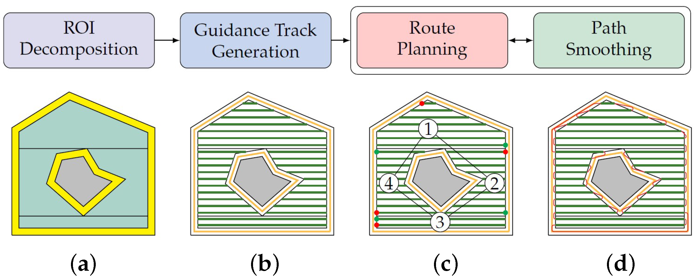
In this work, we expand upon this concept through a comprehensive procedure consisting of four key components, as depicted in
Figure 1. We start by applying a well-established approach for agricultural field processing, the
ROI decomposition. This involves the segmentation of the field into two distinct regions: the headland area and the interior field, as visualized in
Figure 1a. The interior field is subsequently divided into simple cells. Next, we carry out
guidance track generation to delineate the fixed track system to be followed in the path generation process, visualized in
Figure 1b.
Subsequently, two tasks are carried out. Firstly, determining the order in which cells and their corresponding tracks are to be processed is addressed in the
route planning step, visualized in
Figure 1c. Secondly, to transform the information about tracks and their traversing order into a smooth traversable path, the
path smoothing step is employed, which can be seen in
Figure 1d. It is important to emphasize that these two steps are interdependent and are executed parallel to each other, instead of strictly sequentially. The overall methodology for this can be found in the subsequent
Section 3.
1.1. Problem Statement
The problem addressed in this work is the development of a solution strategy for the CCPP problem, with a specific focus on ground-based agricultural machines. Furthermore, the problem is classified as two-dimensional and single-robot, i.e., we assume a single machine moving in a two-dimensional environment. Ensuring universal applicability of this process, the utilized methods are independent of specific dynamic machine models. The only fundamental parameters under consideration are the working width w and the minimum turning radius , both of which are essential in guiding the computations. Our approach involves two objectives: the number of turning maneuvers should be minimized, as well as the overall path length. Since the execution of a turning maneuver is more energy and time consuming than moving along a straight line, the number of turning maneuvers should be minimized in the first place, which also implicitly minimizes operation time. Afterwards, the path should be calculated with a minimal path length, adhering to the path constraints. These constraints include achieving a path smoothness of at least continuity, i.e., continuous curvature, and fulfilling the curvature constraint, with the maximum curvature . To set the geometric boundaries for this problem, it is assumed that the ROI is equivalent to the workspace, thereby restricting the machine’s movement to the confines of the ROI. The ROI is defined as a two-dimensional polygonal area with a single outer boundary, within which non-self-intersecting obstacles are entirely contained.
Our goal is to produce a round-trip complete coverage path, eliminating the need for a specific start and end position. This is aligned with the CTF approach by utilizing a fixed guidance track system. To ensure this, a four-step methodology has been developed, previously described and visualized in
Figure 1, which will be detailed in
Section 3. While all stages of the methodology are discussed, particular emphasis is placed on the combined
route planning and
path smoothing approach, representing the core of this work. The key challenge to be addressed is the computation of both an optimal cell traversing sequence, as well as the calculation of the optimal entry and exit points for the path within each cell. This problem is encoded as a generalized traveling salesman problem (GTSP), providing a structured framework for finding the optimal solution. Additionally, an algorithm is presented to compute an overall smooth and curvature-constrained coverage path out of this discrete traversing sequence, ensuring that the defined constraints are met. This paper exclusively focuses on the coverage paths within the interior field. Solutions for smooth headland paths are provided in a separate work [
11].
1.2. Main Contributions
The main contributions of this work are summarized as follows:
Comprehensive CCPP pipeline: We present a systematic assembly of the complete CCPP pipeline, tailored for agricultural machines, in a versatile and machine-agnostic manner. The approach incorporates considerations such as smoothness and curvature constraints, which are essential for efficient path tracking control for autonomous nonholonomic agents. We introduce optimization methods at various stages of the pipeline, enhancing the generation of precise and efficient coverage paths for agricultural machinery.
GTSP-based route planning: In this work, we address the route planning problem in CCPP by formulating it as a GTSP. Contrary to other works that usually consider the cell-traversal sequence either using the centroid of each cell as a reference [
13,
14] or having fixed entry and exit points, in our work, we additionally optimize entry and exit points for each cell, which can have a significant effect on path length for large-scale agricultural ROIs.
Inter-region path computation: This work also addresses the computation of inter-region paths, an area that has received limited attention in the existing literature. We present an algorithm that first creates feasible piecewise linear paths and subsequently smooths them using NURBS curves. The weights of these curves are optimized such that the path length is minimal while complying with smoothness and curvature constraints.
In summary, these contributions propel the state-of-the-art in CCPP for agricultural machines by delivering a comprehensive and adaptable approach to path planning while also addressing previously unexplored challenges in the field.
1.3. Structure of the Work
The paper is structured as follows. In
Section 2, we begin with an overview of related publications in the field. In
Section 3, we detail the four-stage methodology developed and utilized in this paper. Each of the four stages will be explored in more depth in the subsequent sections.
Section 4 focuses on the ROI decomposition and the generation of the guidance track system. In
Section 5, we explain the generation of smooth and curvature-constrained intra- and inter-region paths.
Section 6 details the route planning step, where we translate the problem into a GTSP. This section elucidates how the results from the previous stages are employed to compute an optimal cell traversing sequence and determine optimal entry and exit points for each cell. Finally, in
Section 7, we implement and evaluate our proposed approach on real agricultural fields. We present our findings and conclusions in
Section 8, along with insights into potential areas for further research.
2. Related Works
Several studies have addressed the complete coverage path planning (CCPP) problem in various agricultural and surveying applications using diverse algorithms and optimization techniques. The topic of guidance track generation has been treated extensively in the review [
15] and references therein. In [
16], an evolutionary neighborhood discovery algorithm for route planning in multiple agricultural fields with obstacles was introduced. The objective function minimized the sum of included edges, the tour distance between fields, machine travel to and from the depot, and the distance between the first and last track to be harvested. In the context of surveying disjointed areas with unmanned aerial vehicles (UAVs), the optimization of visiting order and flight line orientation was tackled by [
17]. The authors applied the rural postman problem to determine the most efficient routes for UAV surveying. In [
13,
14], CCPP for multiple cleaning robots using flow networks was explored. The work employed cellular decomposition to divide the cleaning area into cells and developed an efficient covering order based on the distance between cell centroids. In another study [
18], the authors generalized the boustrophedon variant for UAV area decomposition using Morse functions. The cells were categorized into two classes to create a cell set more suitable for the traveling salesman problem (TSP). Genetic algorithms and TSP algorithms were employed to obtain the shortest path around the cells. The work [
19] focused on applying CCPP to the inspection of disjointed areas. The problem was divided into two phases: inter-region and intra-region path planning. For inter-region path planning, a connectivity graph represented the multiple disjoint regions, and two novel approaches based on mixed integer linear programming (MILP) and heuristics were proposed to generate the ordered sequence of regions to be traversed. Intra-region path planning involved decomposing each region into a grid and planning boustrophedon motion over each region.
The review presented in [
20] provided an overview of various path smoothing techniques applied in robot navigation. While this work dealt with generating smooth paths for all kinds of robot motion, the techniques mentioned, such as interpolation-based smoothing, splines, smoothing based on special curves such as Dubins or Reed–Shepp [
21,
22], and optimization-based smoothing, are directly applicable to complete coverage planning. The problem of generating smooth paths for nonholonomic vehicles in agricultural fields can be broadly categorized into two classes. The first deals with creating smooth headland tracks, wherein typically, a set of points forming a polygon are used to generate a continuous curvature path. Ref. [
11] explored the utilization of weight-optimized NURBS (non-uniform rational B-spline) curves to generate such smooth headland tracks. By optimizing the curve weights, this work ensured that the path followed the polygon track as closely as possible while maintaining the curvature constraints of the system.
The second class of smoothing techniques deals with generating smooth turns connecting two interior tracks. In [
10], an approach to automatically generate smooth turning paths for nonholonomic vehicles in headlands is introduced. This approach considered variable speed profiles and actuator dynamics, allowing for a complete path from the initial to the final state. In [
23], a multi-objective cost function was presented that integrated the additional costs of the yaw angle, curvature, reversing, and path length of self-driving agricultural vehicles, which, combined with the heuristic function of Reeds–Shepp curve length, generated a comprehensive priority value, which could ensure the generated paths were continuous and smooth. In [
24], an algorithm for generating smooth complete coverage paths is proposed, that utilized clothoid curves, allowing nonholonomic mobile robots to move in optimal time. In [
9], the authors presented a method that generated headland turns for parallel tracks with continuous-curvature paths. Nine headland turn maneuvers were provided with minimal computational time.
3. Methodological Approach
In this section, we present a detailed overview of the four-step methodology developed for addressing the CCPP problem tailored to ground-based agricultural machines. The unique challenges posed by these heavy and nonholonomic machines, due to their weight and steering constraints, necessitate a structured approach to coverage path planning. The core principle underlying the CTF concept is the establishment of fixed guidance tracks in the field that agricultural machines will follow, minimizing soil compaction. The methodology developed in this work is based on this concept to address the specific agricultural challenges, and the four key components are presented in the following. Furthermore, the workflow shown in
Figure 2 will guide the reader through these key components.
ROI decomposition: The first step of our methodology involves ROI decomposition. In this phase, the field is divided into two primary zones: the headland area and the interior field. The headland area, situated along the field’s periphery, is designated for machine maneuvers and turns. Its width is determined based on machine-specific parameters, including the minimum turning radius and working width. The interior field, which constitutes the central area of the ROI, undergoes further division. We apply a polygon cell decomposition method to create simple cells, which serve as foundational units for subsequent path planning and coverage optimization. This ensures the division of the interior field into parts that are uninterrupted by obstacles and therefore continuously traversable, simplifying the planning process of coverage.
Generation of guidance tracks: Following ROI decomposition, the CCPP process proceeds with the generation of a guidance track system. This system guides the final coverage path to achieve full field coverage and is categorized into headland guidance tracks and interior guidance tracks. Headland guidance tracks are positioned within the headland area, with their number contingent on the area’s width and the working width w. Additionally, each cell resulting from the ROI decomposition is filled with parallel interior guidance tracks, spaced at a maximum distance of w. The desired coverage path closely follows this track system, playing a crucial role in ensuring organized and efficient field coverage.
Route planning: Route planning holds significant importance in CCPP, particularly in determining the most efficient sequence for navigating the generated interior guidance tracks. It involves determining the order in which cells are traversed and sequencing tracks within each cell. In this work, we assume a sequential order of the tracks inside each cell. We focus on the computation of an optimal cell-traversing sequence along with the entry and exit points for each cell. The primary objective is to establish a sequence that minimizes travel distance while ensuring systematic coverage of the entire field.
Smooth path planning: This stage of the CCPP process focuses on generating smooth and drivable coverage paths based on the guidance tracks and a traversal sequence. This includes the generation of both intra-region paths for smooth coverage within a single cell and inter-region paths that connect two intra-region paths. The aim is to guarantee that agricultural vehicles can navigate the field without abrupt movements by ensuring continuous curvature and considering the curvature constraint. This minimizes the potential for soil compaction, resource wastage, and stress on the machinery. An additional aspect of this stage involves the generation of smooth headland paths based on the headland tracks. Since our focus is primarily on the interior coverage paths, further details on headland path generation can be found in [
11].
The ROI decomposition and the generation of the guidance track system are closely related and will be covered in this work together in
Section 4. As seen in
Figure 2, the stages of
route planning and
smooth path planning are closely interconnected. The smooth intra- and inter-region paths are utilized in the problem formulation of the route planning process to be able to compute an exact objective function, namely the path length. Consequently,
Section 5 first addresses the smooth path planning before delving into the overall route planning stage in
Section 6.
In summary, the algorithm employed in this study is outlined in Algorithm 1. The algorithm is structured into distinct phases: lines 1–2 encompass the ROI decomposition process, while lines 3–6 pertain to the creation of the guidance track system, both detailed in
Section 4. Line 7 delineates the route planning and path smoothing steps, detailed in
Section 5 and
Section 6 and Algorithm 3.
| Algorithm 1 Complete coverage path planning algorithm. |
Input: Region of onterest (ROI), working width w, minimum turning radius Output: Smooth and curvature-constrained coverage path of ROI - 1:
Split ROI into headland area and interior field - 2:
Decompose the interior field into simple cells - 3:
Generate headland tracks - 4:
for cell in decomposition do - 5:
Generate interior guidance tracks - 6:
end for - 7:
return Algorithm 3
|
4. ROI Decomposition and Guidance Track Generation
This section provides a concise overview of the essential components of the ROI decomposition and guidance track generation process. A comprehensive review of these topics can be found in [
15]. The initial step involves the separation of the headland area from the interior field. This is followed by the cellular decomposition of the interior field and a brief overview into the method employed for the generation of interior guidance tracks applied to each of the resulting cells.
4.1. Headland Area Separation and Headland Guidance Tracks
The general approach starts with the classification of the ROI, dividing it into the headland area and the interior field, as visualized in
Figure 1a. To separate the headland area from the interior field, polygon offsetting techniques [
25] have proven valuable, employing an inward offset of the outer boundary and outward offsets of the obstacles. This technique can be applied for generating the headland guidance tracks covering the headland area, visualized in
Figure 1b (orange). For a solution that addresses several options for handling the polygon corners, Clipper2 [
26] is a promising library that offers a versatile toolkit for polygon offsetting (and clipping). More details can be found in [
15].
4.2. Cellular Decomposition of Interior Field and Interior Guidance Tracks
A widely used approach for exact cellular decomposition, particularly in CCPP, is based on a line sweep algorithm. This approach utilizes a sweepline that sweeps over the ROI, detecting specific events, and inserts lines parallel to the sweepline at these events to decompose the region, as visually demonstrated in
Figure 3. One straightforward example of this technique is
trapezoidal decomposition [
27], visualized in
Figure 4a. In this case, all polygon vertices are considered events, which can result in numerous narrow cells. Another prominent and effective sweepline-based decomposition technique is the
boustrophedon cellular decomposition (BCD) [
28], which is illustrated in
Figure 4b. The main idea behind this technique is to generate cells that can be covered using a back-and-forth motion, resulting in a smaller number of cells compared to trapezoidal decomposition. The cells are monotone polygons with respect to the sweep direction, enabling individual coverage by a simple back-and-forth motion with tracks parallel to the sweepline. This technique was initially introduced in [
28] and later extended in [
29]. The BCD finds widespread application in various fields, such as multi-robot complete coverage path planning [
30], efficient point-to-point path planning [
31], inspection with UAVs [
32], harbor seabed surveys with AUVs [
33], and achieving minimal path length [
34].
In this paper, we adopt the BCD method, following the recommendation in [
15], to decompose the ROI into simple, in this case monotone, cells. The angle of the sweepline is treated as a variable that allows us to determine the optimal decomposition. To achieve this, we focus on optimizing the number of turning maneuvers, specifically the number of interior guidance tracks, as they significantly impact the path execution cost [
35]. The optimization process involves evaluating the minimum sum of altitudes of the resulting cells for various sweepline directions. The mathematical formulation of this optimization can be found in [
15].
Once the area is successfully and optimally decomposed, each resulting monotone cell is covered with straight parallel interior guidance tracks with a distance of less than or equal to
w, parallel to the utilized sweepline for the decomposition. Due to the fact that the cells are monotone with respect to the sweepline direction, covering the cells in such a back-and-forth manner is possible and straightforward. This is illustrated in an example in
Figure 1b.
5. Smooth Path Planning
Smooth path planning plays a crucial role in robot navigation, particularly for larger machines with significant minimum turning radii, ensuring both machine and soil stability during operations. The overall path in our approach consists of two distinct path types:
Intra-region paths, responsible for covering a single cell resulting from the cellular decomposition and following the interior guidance tracks, primarily focusing on managing turning maneuvers between tracks;
Inter-region paths connecting the intra-region paths of two different cells aligned with the track system, including both interior and headland tracks.
These two different path types are visualized in
Figure 5. The next section describes the computation of both types of paths, employing various smoothing techniques to ensure seamless and efficient traversal for the machine.
5.1. Intra-Region Path
The aim of intra-region path planning is to compute trajectories for turning maneuvers from one guidance track to another. The traversing order of the tracks within a single cell also presents an opportunity for optimization. In this paper, however, we will adopt a sequential track traversing order for simplicity and ease of implementation. Notably, research in the literature demonstrates that the traversing order of tracks within a cell can indeed be optimized for improved efficiency and coverage [
16,
36,
37,
38].
Each turning maneuver can be computed independently and needs to satisfy the continuous curvature (CC) constraint to account for the finite steering speed of the machine. This is realized by computing trajectories for the CC Dubins model [
21] from a given start configuration
to an end configuration
. A configuration
is defined by the pose
and curvature
. The mathematical description of the CC Dubins model is given by the differential equation system [
21]
where the control inputs
v and
correspond to the driving velocity of the rear wheels and the angular acceleration, respectively. Thereby,
is related to
, the steering velocity of the front wheels. Together with the wheelbase
b, the following relation holds [
21]:
The states of this model are visualized in
Figure 6. The CC Dubins model assumes a constant unit-driving velocity and upper bounds on the curvature and angular acceleration due to real-world steering limitations (the steering angle
is mechanically limited, s.t.
)
This CC Dubins model is an extension of the regular Dubins model [
39], where the continuity of the curvature was not a condition. The aim is to find a continuous-curvature planar curve following (
1) that connects two points
in the plane with prescribed tangents
and curvatures
. The curve must satisfy the curvature and curvature derivative bounds from (
3). The configurations
are determined by the exit pose of the current track and the entry pose of the next track, subject to the constraint of zero curvature at both the beginning and end of the maneuver, to ensure the continuous curvature’s transition into a straight guidance track. This is sketched in
Figure 7.
The utilization of this model ensures that the resulting path maintains continuous curvature and adheres to the necessary curvature constraint. This flexibility underscores the model’s suitability for a wide range of agricultural machines, contributing to its practical applicability.
Based on these specifications of the maneuver, we formulate an optimal control problem with the objective of minimizing the path length. To efficiently solve such optimal control problems, we can leverage software libraries such as TransWORHP [
40], which offer robust capabilities in trajectory planning and optimization, based on the ESA NLP solver WORHP [
41]. Additionally, a specialized alternative for this specific scenario is the software library hbanzhaf/steering_functions [
22], which is tailored specifically for computing CC Dubins curves. Both libraries provide effective methods to find trajectories that adhere to curvature constraints while optimizing the path length, thereby facilitating successful intra-region path planning using the CC Dubins model.
The study of different turn types within the agricultural context is well-documented in references such as [
9,
10,
42], offering a comprehensive overview of available techniques. Notable turn maneuvers are visually presented in
Figure 8, and these maneuvers significantly influence the efficiency and precision of agricultural vehicle path planning. In specific situations,
-turns exhibit shorter turning distances compared to hook-turns, although the latter require less headland width. The choice between these turn types may be influenced by farmers’ preferences. Overall, when
is satisfied, (flat) U-turns are optimal, while
- or hook-turns are preferred when this condition is not fulfilled.
The entirety of an intra-region path is composed of a sequence of the described turning maneuvers. Illustrative representations of these intra-region paths can be found in
Figure 5 (red), where the paths are also connected by inter-region paths (blue). These inter-region paths serve to establish continuity and transition between successive intra-region paths.
5.2. Inter-Region Path
The inter-region path is a critical component that connects the end of one intra-region path with the beginning of another. This path must possess essential properties, including staying within the ROI to avoid obstacles, primarily following the guidance tracks (both headland and interior) to minimize the soil compaction, and being relatively short to optimize overall operational time. Achieving smoothness, i.e., continuous curvature, is also necessary for seamless machine operation. To address these requirements, our approach involves generating an initial piecewise linear inter-region path. Subsequently, we employ non-uniform rational B-spline (NURBS) curves, incorporating weights in each control point [
43]. With these, we smooth out the piecewise linear path while considering curvature constraints through weight optimization, similar to the approach described in [
11].
5.2.1. Piecewise Linear Inter-Region Path
The algorithm for computing a piecewise linear inter-region path
is presented in Algorithm 2, with a visual representation of the steps provided in
Figure 9. Its primary objective is to establish a connection between two intra-region paths.
The algorithm initiates by examining whether the end track of the first and the start of the second intra-region paths are neighboring and can be directly connected with a simple CC Dubins turn, as elaborated upon in the previous section. This connection, illustrated in
Figure 5 (upper right corner and second inter-region path on the lower left), is characterized by its smooth and minimal curvature. However, if a direct connection is not feasible, the algorithm extends both the start and end tracks, as demonstrated by the dashed black line in
Figure 9. These extensions result in intersections with the headland tracks, marked as red dots in
Figure 9. Subsequently, for each combination of intersections (one from the start track extension and one from the end track extension), when they correspond to the same headland track, the path is further optimized, as summarized in lines 6–13. To ensure the inter-region path’s feasibility concerning the ROI, specifically in terms of obstacle avoidance, the algorithm refines it by incorporating detours around the obstacles using the headland tracks. Furthermore, in cases where transitions from one headland track to another are encountered, the algorithm seeks to align the path with the interior guidance tracks, thereby minimizing soil compaction in that area. This results in the formation of two sub-paths, each connecting the start or end track with the same headland track. These two sub-paths are then conjoined to create a path candidate for the piecewise linear inter-region path. Importantly, this process is repeated for all intersection combinations, and in the end, the algorithm selects the path candidate with the shortest overall path length. The algorithm ensures that
remains within the ROI and traverses along the headland and interior guidance tracks. This approach effectively creates an efficient and feasible piecewise linear inter-region path for transitioning from one cell to the other.
| Algorithm 2 Piecewise linear inter-region path. |
Input: Starting interior track at point , ending interior track at point , headland guidance tracks the path should be aligned with Output: Piecewise linear inter-region path connecting and - 1:
if and are neighboring tracks && and are close then - 2:
return CC Dubins turn from to - 3:
end if - 4:
Extend track at and at - 5:
Compute the sets of intersections resulting from the extensions of intersecting with a track of - 6:
for in do - 7:
if and are on different tracks in then - 8:
continue - 9:
end if - 10:
Refine the straight connection between the initial points and the intersection points such that the path conforms to the contours of all tracks in . - 11:
if Refining results in transitioning between different tracks of then - 12:
Align the path with the closest interior guidance tracks, if possible. - 13:
end if - 14:
This results in two sub-paths, each starting at or and concluding at the same headland track - 15:
Combine these paths, including in-between points along the headland track, to construct a path candidate. - 16:
end for - 17:
return Path candidate with minimal length
|
The subsequent stage involves smoothing this path to ensure the drivability of the path by nonholonomic vehicles with curvature constraints. To achieve this, we employ NURBS curves, following the idea of [
11].
5.2.2. Non-Uniform Rational B-Spline (NURBS) Curves
NURBS curves serve as generalizations of both B-splines and Bézier curves, sharing a definition based on a set of control points
and a knot vector
. However, the main distinction lies in their rationality, arising from the incorporation of weights
associated with the control points [
43,
44]. A NURBS curve of degree
with weights
w is defined as
, with
with the domain
, and
the
i-th basis function of degree
p [
43]. In this study, we employ a uniform knot vector, a widely used approach in NURBS curve implementations [
43]. Leveraging NURBS curves grants us significant flexibility in achieving the desired level of smoothness as we can freely select the degree
p to suit our specific needs. Utilizing a uniform knot vector ensures that a NURBS curve of degree
p attains
continuity, providing a smooth trajectory. However, when choosing the degree of the curve, it is crucial to strike a balance between achieving the desired smoothness and managing computational costs, as higher degrees result in increased computational complexity.
5.2.3. Smoothing Inter-Region Paths Using NURBS Curves
To achieve a smooth and continuous inter-region path while satisfying the curvature constraint, we draw inspiration from the approach proposed in [
11]. The NURBS (non-uniform rational B-splines) curve’s weights are optimized to adapt its shape, ensuring compliance with the curvature constraint. The path points of the piecewise linear inter-region path
are employed as control points, or the path is further discretized to have an equal step size. We then solve a nonlinear optimization problem to compute the optimal weights
w. Denoting the squared Euclidean distance between a point on the NURBS curve
and the closest point on
as
for
, and representing the corresponding curvature in this point of the NURBS curve as
, the formulation of the nonlinear optimization problem is as follows:
The objective function ensures that the resulting NURBS curve closely follows the piecewise linear path
. Simultaneously, the constraint ensures that the curvature remains within the predefined upper bound
. This nonlinear optimization problem is solved using the ESA NLP solver WORHP [
41], allowing us to obtain a smooth inter-region path that adheres to the curvature constraint.
6. Route Planning
Route Planning deals with determining the optimal traversing order of individual cells, resulting in a complete coverage path with minimized length that consists of a sequence of intra- and inter-region paths. To address this optimization challenge, we formulate it as a graph problem, wherein the nodes represent intra-region paths, and the edges represent the inter-region paths. Specifically, we cast this problem as a generalized traveling salesman problem (GTSP) and formulate it as an integer program. Subsequently, we demonstrate how to encode the different paths into nodes and edges, enabling us to apply the GTSP technique to our specific problem. By transforming the coverage path planning into a graph-based optimization problem, we aim to efficiently determine the most effective order for traversing cells, ultimately leading to a highly optimized and shortened path for complete coverage.
6.1. Generalized Traveling Salesman Problem (GTSP)
The traveling salesman problem (TSP) is a classic optimization challenge involving a complete graph, aiming to find the cheapest Hamiltonian cycle that visits every node exactly once. Its practical relevance in logistics, transportation, and network design has led to the development of various efficient solution methods [
45,
46,
47,
48,
49], despite its computational complexity for large instances.
In contrast, the generalized traveling salesman problem (GTSP) is a TSP variant where nodes are organized into clusters. The goal is to discover an optimal Hamiltonian cycle visiting one node from each cluster. This cluster-based structure sets the GTSP apart from the standard TSP, making it valuable in scenarios requiring optimized routes across multiple location subgroups [
50,
51].
The graph representing the GTSP is defined as
, with
representing the set of nodes and
representing the set of edges, each assigned with costs. The nodes are partitioned into
m distinct clusters
, with
for
. By utilizing binary variables, a GTSP can be formulated as an integer linear program. Thereby, the costs of the generalized cycle are minimized. The Gurobi optimizer [
52] excels in integer linear programming due to its efficient treatment of sparse linear algebra, precise numerical error management, and effective heuristic strategies. SCIP [
53] is another fast solver for mixed integer programming and nonlinear programming, doubling as a framework for constraint integer programming and branch-cut-and-price. In this work, we will utilize the Gurobi optimizer.
6.2. Optimal Cell-Traversing Sequence Using GTSP
The primary optimization objective of our approach is to minimize the overall path length while ensuring each cell is covered exactly once. Encoding the problem as a GTSP involves defining the nodes of the graph, along with the edges and their associated costs. This approach intricately intertwines the concept of smooth path planning with the route planning aspect, as visualized in
Figure 1. The route planning and smooth path planning stage is summarized in Algorithm 3.
The first step is to introduce the representation of nodes. There are four distinct ways to cover a single cell with an intra-region path utilizing the given parallel guidance tracks, as illustrated in
Figure 10. It is assumed that the start and end tracks are the two outermost ones. Each of these possibilities is translated into a node within the graph. Consequently, each node possesses a specific intra-region path, delineated by a designated start and end track and position. Furthermore, the four nodes corresponding to the same cell are clustered together. If the cellular decomposition yields a total of
m cells, the graph will comprise a total of
n = 4
m nodes and
m clusters.
Edges connecting two nodes are represented by the linear inter-region path that connect the corresponding two intra-region paths. The cost of this edge is defined by the sum of the length of the piecewise linear inter-region path and the length of the intra-region path of the preceding node. This cost function matches the aim of minimizing the overall path length.
Constructing this graph enables the formulation of an integer program to solve the GTSP, ultimately resulting in the identification of a Hamiltonian cycle. This cycle furnishes an optimal sequence of nodes and edges. Decoding them back yields a sequence of intra-region paths and piecewise linear inter-region paths. After smoothing the latter, as described in
Section 5.2.3, these paths can be concatenated consecutively, yielding a smooth and curvature-constrained coverage path.
Notably, during the GTSP solution process, it is imperative to compute the costs associated with all inter-region paths connecting various cell combinations. To enhance computational efficiency, it is feasible to consider only the piecewise linear path
in this optimization step. The computation of the smooth inter-region path can be deferred to the final step when establishing the complete coverage path. This approximation remains valid, as the smoothing process has a minimal impact on path length. Similarly, for intra-region paths, their length does not significantly influence the optimization results and can be managed accordingly. This streamlined approach ensures both computational efficiency and the derivation of an optimal coverage path.
| Algorithm 3 Route planning and smooth path planning |
Input: Fixed guidance track system, minimum turning radius , track width w Output: Optimal coverage path - 1:
for cell in cells do - 2:
Create a cluster of four nodes from the track system by calculating the four intra-region paths for the cell - 3:
end for - 4:
for pair of nodes in distinct clusters do - 5:
Calculate the piecewise linear inter-region path - 6:
Create an edge connecting the two nodes - 7:
Assign costs to the edge: Sum of the lengths of the inter-region path and the intra-region path of the first node - 8:
end for - 9:
The clustered nodes and edges correspond to a GTSP. Formulate the linear program and use solver to compute the solution - 10:
The solution is an optimal sequence of nodes (and their connecting edges). - 11:
Encode the nodes and edges back to intra- and piecewise linear inter-region paths, resulting in a path vector - 12:
for path in pathvector do - 13:
if path is inter-region path then - 14:
Smooth path using NURBS curves - 15:
end if - 16:
Append path to final coverage path - 17:
end for - 18:
return final coverage path
|
7. Results and Discussion
Within this section, we present the outcomes of our path planning methodologies. Since we have opted for a well-established polygon decomposition technique, we do not provide an evaluation of the ROI decomposition and guidance track generation steps. Notably, our modular approach allows for flexible interchangeability of the chosen decomposition method without affecting the subsequent steps. The evaluation focuses on the smoothing phase, encompassing both intra- and inter-region paths. We examine example paths, studying the impact of varying maximum curvatures on these trajectories. Subsequently, we apply our proposed path planning methodology to four distinct real-world agricultural fields. Through this application, we seek to assess the efficacy of the curvature constraint coverage paths generated by our approach. Afterwards, we present a comparative analysis between our GTSP-based route planning algorithm and a heuristic approach to underscore the advantages of the former.
7.1. Effects of Varying Curvature Constraints on Smooth Path Planning
We will first focus on the intra-region paths, considering (flat) U-turns and
-turns. Employing the TransWORHP software library [
40], we solve the optimal control problem characterized by (
1) and (
3).
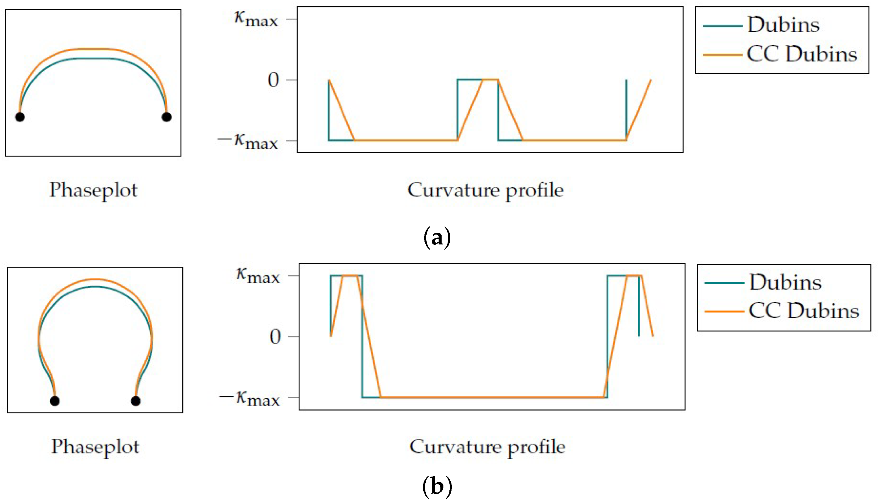
Figure 11 provides a visual comparison demonstrating the quantitative disparity between a conventional Dubins curve [
39] and a CC Dubins curve, specifically in the case of a flat U-turn and an
-turn. Furthermore, the characteristic curvature profile of these two turn types can be seen. While the path length of the CC turn slightly exceeds that of the traditional Dubins curve, the pronounced difference lies in the continuity of the curvature profile.
A comprehensive assessment encompassing various maximum curvatures
for the same maneuver and both turn types is illustrated in
Figure 12 and
Figure 13. The inspection of curvature profiles reveals a consistent presence of seven phases within the curves. Notably, three phases maintain constant curvatures at values
or 0, representing motion on a circular arc or straight line, respectively. A continuous transition between these curvature values is realized by introducing a slope of
to the curvature increments/decrements, resulting in clothoid arcs. This characteristic differentiates these CC Dubins paths from regular Dubins curves.
In order to shed light on the inter-region path smoothing, an illustrative example is showcased in
Figure 14b. This visual representation includes both the piecewise linear path
(depicted in black) and the smoothed paths calculated by weight-optimized NURBS curves for varying maximum curvatures
. The weight optimization process is solved by the ESA NLP solver WORHP [
41]. In this, a smoothness degree of
is employed, resulting in a curve
. This characteristic is also evident in the continuous and differentiable curvature profile. Both the phase plot and the curvature profile underscore the remarkable conformity of the resulting inter-region paths with the piecewise linear path while simultaneously adhering to the curvature constraint. It is important to emphasize that during the inter-region path smoothing, the objective is not merely to achieve the shortest path but rather to closely adhere to the piecewise linear path.
7.2. Application of the Optimal CCPP Algorithm to Real Agricultural Fields
In this section, we present the results of applying our method to four distinct real agricultural fields, with field data provided by NEXAT GmbH [
54]. To ensure better comparability, the fields were rescaled to similar dimensions, and the GTSP was solved using the Gurobi software, version 10.0.1 [
52]. The specifications of the considered fields and the resulting coverage paths are summarized in
Table 1 and visually depicted in
Figure 15,
Figure 16,
Figure 17 and
Figure 18.
However, a visual examination of the results may at times appear unconventional to observers unfamiliar with our methodology. This is primarily due to two reasons. First, our objective is to calculate a round-trip coverage path, and second, the inter-region paths are not always equivalent to the most direct straight-line connections. As a result, the optimal solution might not always align with intuitive expectations.
Computation times for our approach vary depending on the complexity of the field, ranging from milliseconds for Fields 1, 2, and 4 to a few minutes for Field 3. Since our primary focus is offline path planning within a known environment, as long as the computation time does not exceed several hours, it does not play a significant role.
Interpreting the efficiency of these outcomes can be challenging. For instance, solely considering path length may not provide a comprehensive evaluation of the overall path quality. Even though the considered optimization criteria is the minimization of the path length, to be able to further evaluate and compare the results, looking only at the path length without additional context is not recommended. Due to the guidance track system, the length of the intra-region paths can only be changed to some extent. Furthermore, as the inter-region paths are primarily for traversal between cells, and the actual field processing is handled by the intra-region paths, minimizing the length of the inter-region paths is desirable. To address this challenge, we introduce two distinct metrics. First, we compute the
ratio of the covered area (CA) using the formula
This ratio, which naturally exceeds 1 due to the design of the interior tracks ensuring complete coverage of the inner field, is desired to be minimized. It corresponds to the overlapping areas in the interior field and the paths along the headland. As observed in
Table 1, the area attributed to turns and inter-region paths hovers around 10–15%. This percentage is highest for Field 3, which has the most obstacles and resulting cells, necessitating a higher number of inter-region paths, thus increasing the amount of overlapping areas of the path and paths inside the headland area.
Second, we introduce the
inter-region path ratio (IR), defined as
A smaller value of IR signifies a more favorable outcome, indicating that less path is used for traversing between cells and more for actual field processing. The tabulated results in
Table 1 demonstrate that this ratio varies from 2.4 to 6.0%, underscoring the effectiveness of our method in maintaining shorter inter-region paths. As expected, the number of cells resulting from the decomposition directly impacts the amount of connection paths required.
7.3. Comparison of GTSP-Based Route Planning with a Heuristic Approach
In this section, we present a comparative analysis between the GTSP-based route planning approach proposed in this paper and a heuristic alternative. While the overall methodology, including the ROI decomposition, and the computation of intra- and inter-region paths remains consistent, the key difference between the two approaches lies in how the cell-traversing sequence is computed. For the evaluation, we use Fields 1 to 4 from
Figure 15,
Figure 16,
Figure 17 and
Figure 18.
The GTSP-based approach, which has been detailed in this paper, is the first method under consideration.
For the heuristic approach, we utilize the same node creation method as for the GTSP-based approach. This means that for a decomposition resulting in m cells, nodes are created, where each node represents a covered cell and the start position of the intra-path within that cell. Starting from a specified cell with a predetermined start track and position, a local search identifies the next yet-uncovered node. Thereby, the length of the inter-region path is considered as the cost function. This process continues until all nodes are covered, after which the path returns to the starting point. This results in one heuristic solution. To make a meaningful comparison with our optimal approach, we apply the heuristic method times, accounting for all possible start tracks and positions. Finally, we select the heuristic solution with the shortest overall path length for comparison with our GTSP-based approach.
The results of this comparison are presented in
Table 2. It is evident that the optimal GTSP-based approach consistently outperforms the heuristic local search approach in terms of both the overall path length and the combined length of the interior paths.
The magnitude of the GTSP-based approach’s advantage over the heuristic method varies across the fields. For Fields 1 and 2, the inter-region path length is approximately 13% shorter, showcasing the substantial advantage of the GTSP-based approach. In contrast, Fields 3 and 4 exhibit a more modest difference, with the inter-region path length being only about 2% shorter. This variation highlights the versatility and effectiveness of the GTSP-based approach, which can yield significant improvements in certain scenarios while still providing benefits in others.
8. Conclusions and Future Work
In summary, our study has introduced a comprehensive methodology for generating smooth complete coverage paths in agricultural fields while adhering to critical curvature constraints. This methodology encompasses four essential steps: ROI decomposition, guidance track generation, route planning, and smooth path planning. We have highlighted the modular nature of our approach, making it adaptable to diverse requirements and allowing for the interchangeability of methods within each step. The algorithms presented in this work are designed for easy implementation and understanding.
Through practical applications in real agricultural fields, we have validated the algorithm’s suitability for addressing the unique challenges posed by agricultural environments. The comparative evaluation against a heuristic approach has revealed the advantages of employing a GTSP-based problem formulation in the route planning phase.
It is essential to acknowledge that, as with any approach, our methodology has its limitations. One notable limitation is the relationship between computational effort and the number of cells in the GTSP. As the number of cells increases, the complexity of the GTSP also grows, which can, in extreme cases, lead to infeasibility for certain fields. When dealing with a very large number of cells, even powerful optimization solvers such as Gurobi may struggle to compute a solution within a reasonable time frame. However, it is worth noting that this limitation is generally not a concern for practical agricultural applications. Most agricultural fields tend to be rectangular in shape with relatively few obstacles, keeping the number of cells within a manageable range.
Nonetheless, when dealing with unconventional or irregular field geometries, our approach may face challenges, particularly during the computation and smoothing of the inter-region path. We cannot guarantee that our methodology will be suitable for all possible edge cases given the diverse range of field layouts and conditions. However, for the vast majority of typical agricultural scenarios, our approach remains a robust and efficient solution for coverage path planning. Careful consideration of field characteristics and a well-defined decomposition process can help mitigate these limitations, ensuring the effectiveness of our approach for real-world applications.
However, there are several areas for potential improvement. One limitation we have addressed is the sequential traversal of interior guidance tracks within a single cell and the restricted choice of start and end tracks in each cell. To enhance the algorithm’s efficiency, future work could focus on optimizing the sequencing of tracks within cells and the selection of start and end tracks.
Moreover, a critical aspect that remains to be integrated is the consideration of machine capacity constraints, which is particularly relevant in real-world agricultural scenarios where machines periodically return to a depot for various reasons, such as unloading harvested materials. This addition would involve the computation of multiple round-trip paths, some of which may not cover each cell but are constrained by their total path length and the need to pass through a designated depot location. Integrating this capability would further enhance the practical applicability of our approach, enabling more precise and effective path planning strategies in the field.
Overall, our work provides a strong foundation for addressing CCPP challenges, and we look forward to future developments that build upon these principles for enhanced efficiency and adaptability in agricultural field operations.


