Abstract
Agricultural tractors are subject to lateral forces when traveling on slopes, making it difficult to accurately follow a set course. In this paper, a steering compensation method is first proposed based on the force analysis of a tractor traveling on slopes, which compensates the steering angle according to the friction force and gravity force imposed on the tractor. Further, when traveling on slopes, acceleration and a load applied to the tractor are usually time-varying. To address this problem, this paper proposes a steering compensator that can automatically adjust a compensation coefficient, as well as a design for a model predictive controller with the steering compensator for a tractor. Simulation results show that under different traveling speeds, turning radius, and slope angles, the steering compensator allows the tractor to travel more smoothly, i.e., the distance between the actual traveling route and the reference route fluctuates within a smaller range. Further, during straight-line traveling, the static error can be effectively reduced, i.e., the distance between the actual traveling route and the reference route is closer to zero. Overall, the steering compensator enables the tractor to track the reference route more accurately.
1. Introduction
1.1. Path Tracking Control for a Tractor
In studies of path tracking control for tractors, the most common topic is pure pursuit control, which is based on heading angle and lateral deviations to obtain a steering angle. H. Wang et al. [1] detail a method of directly obtaining the control law in simple form and any relevant parameters. The article addresses some of the problems associated with the application of navigation systems in agriculture, including slow on-line speed, poor on-line stability, and poor adaptability to complex road environments. These problems can be summarized as path tracking and stability problems in cases of large position deviation or large heading angle deviation.
In practical applications, a reference route is often given in the form of a series of points rather than describing it with an ideal equation. As a result, the problem of path tracking is often treated as a problem of point tracking [2]. Some researchers then proposed a method called aiming pursuit control, which involves a model based on the steering pattern of a driver when driving a tractor. During straight-line tracking, a driver will aim at a point on the reference route in front of the tractor and then control the tractor toward that point by steering. In order to accurately track curved paths, many researchers have proposed a variety of dynamic adaptive methods for forward-looking distance and target point [3,4,5,6,7].
The principle of a PID (proportional–integral–derivative) controller is simple, intuitive, and very easy to use, and the related theory is very mature. As a result, it has long been used in industrial control. Although there are large limitations when PID is used in time-varying and nonlinear systems, generally satisfactory control results can be obtained after reasonable parameterization. Therefore, a number of researchers have designed navigation controllers based on PID [8]. Many studies have similarly used PIDs as navigation controllers and utilized performance metrics to parameterize controllers [9,10,11,12]. J. Hu and T. Li [11] use a linear quadratic regulator based on minimizing system error and error variation to determine the optimal parameters of a PID navigation controller. M. Zhang et al. [12] also designed and tuned a PID controller with the same approach and used a proportional controller for steering angle tracking.
Fuzzy control is widely used in the control of nonlinear systems, and it is simple and intuitive to realize the control of a system using existing operating experience. Like the PID controller, it does not require a model and is a kind of model-free control method. Many researchers have designed fuzzy controllers for tractors [13,14,15,16,17,18,19,20,21,22,23]. Z. Liu et al. [13] first obtained the position and attitude of a tractor based on machine vision, then designed a fuzzy controller with lateral and heading deviation as inputs and a desired steering angle as output, and finally used a PID controller to track the desired angle to realize motion control of the tractor.
Model predictive control (MPC) is based on a model of a system and a minimization of an objective function in a finite predictive horizon, using optimization for a control law. It has advantages in that it can easily take into account various constraints of a system as well as being able to make predictions at a certain distance, which is difficult to do with other controllers. A number of researchers have designed model predictive controllers based on linear time-varying models for tractors [24,25,26,27,28,29].
1.2. Path Tracking Control of Tractors on Sloping Roads
Nowadays, a considerable portion of cultivated land has a certain slope, so the development of agricultural equipment and control methods that can adapt to sloping land operations is of great importance for the advancement of agricultural automation. Crawler tractors and tractors with body attitude adjustment mechanisms have been widely studied in order to adapt agricultural machines to sloping land [30]. However, mechanically modifying tractors generally increases the cost of tractor manufacturing and agricultural operations significantly. In addition to focusing on the mechanical design aspects, by improving the existing control methods to make the tractor drive on slopes as close to level ground as possible, this could be an immediate upgrade to many tractors at essentially no additional cost (since it would only require modifying the program code in the original controllers). Therefore, upgrading the control methods of ordinary tractors to accommodate sloping ground may be a better option. The problem to be solved in this paper can be defined as a design of compensation algorithms to make the original controller applicable for controlling tractors traveling on slopes.
Currently, there are relatively few studies related to improving the control performance of tractors when traveling on a slope, but there are some articles that focus on the side-slip phenomenon of tractors. T. Kraus et al. [31] designed a nonlinear model predictive navigation controller for a tractor based on an extended kinematic model that takes into account side-slip. J. Backman et al. [32] developed a kinematic model for a tractor-trailer system considering side-slip effects and designed a nonlinear model predictive controller based on this model to realize tracking control of a trailer. A. Hill et al. [33] first developed an extended kinematic model considering the effect of side-slip and then designed an adaptive nonlinear model predictive control based on this model, which can adaptively optimize control gains on-line in order to achieve better performance.
1.3. Main Contributions of This Paper
Unlike the above-mentioned studies, this paper focuses on the adverse effects of lateral force on a tractor while traveling on a slope and compensates for this lateral force by adjusting a steering angle based on mechanical analysis. To address problems of time-varying loads and time-varying ground-catching forces on tractors in actual use, a steering angle compensation method with an automatically adjusted compensation coefficient is proposed. This method introduces the theory of PID control and determines the compensation coefficient based on a relationship between the actual traveling path of the tractor and a “desired path” estimated based on a kinematic model. Finally, based on a model predictive path tracking control task for a tractor, it is presented how to combine the proposed steering angle compensation method with a model predictive controller to achieve more accurate path tracking. Experimental results show that by introducing the steering angle compensation method proposed in this paper, a tractor can track a reference route more accurately when traveling on a sloping road.
The sections of this paper are organized as follows: The first section focuses on an overview of methods for path tracking control of tractors and methods of controlling tractors for the slipping problem, and a brief description of the method proposed in this paper is given. Section 2 presents the physical principles and specific algorithms of the steering angle compensation method. Section 3 describes a predictive control method that is referenced in this paper. Section 4 presents an algorithm that combines the proposed steering angle compensation algorithm with predictive control and applies it to the task of path-tracking a tractor. Experimental results are given in Section 5. Section 6 summarizes the contents of the paper.
The mathematical notations and their meanings involved in this paper are as follows: The m-dimensional set of vectors is denoted as . For a vector, .
2. Design of Steering Angle Compensators
2.1. Force Analysis of a Tractor Traveling on Slopes
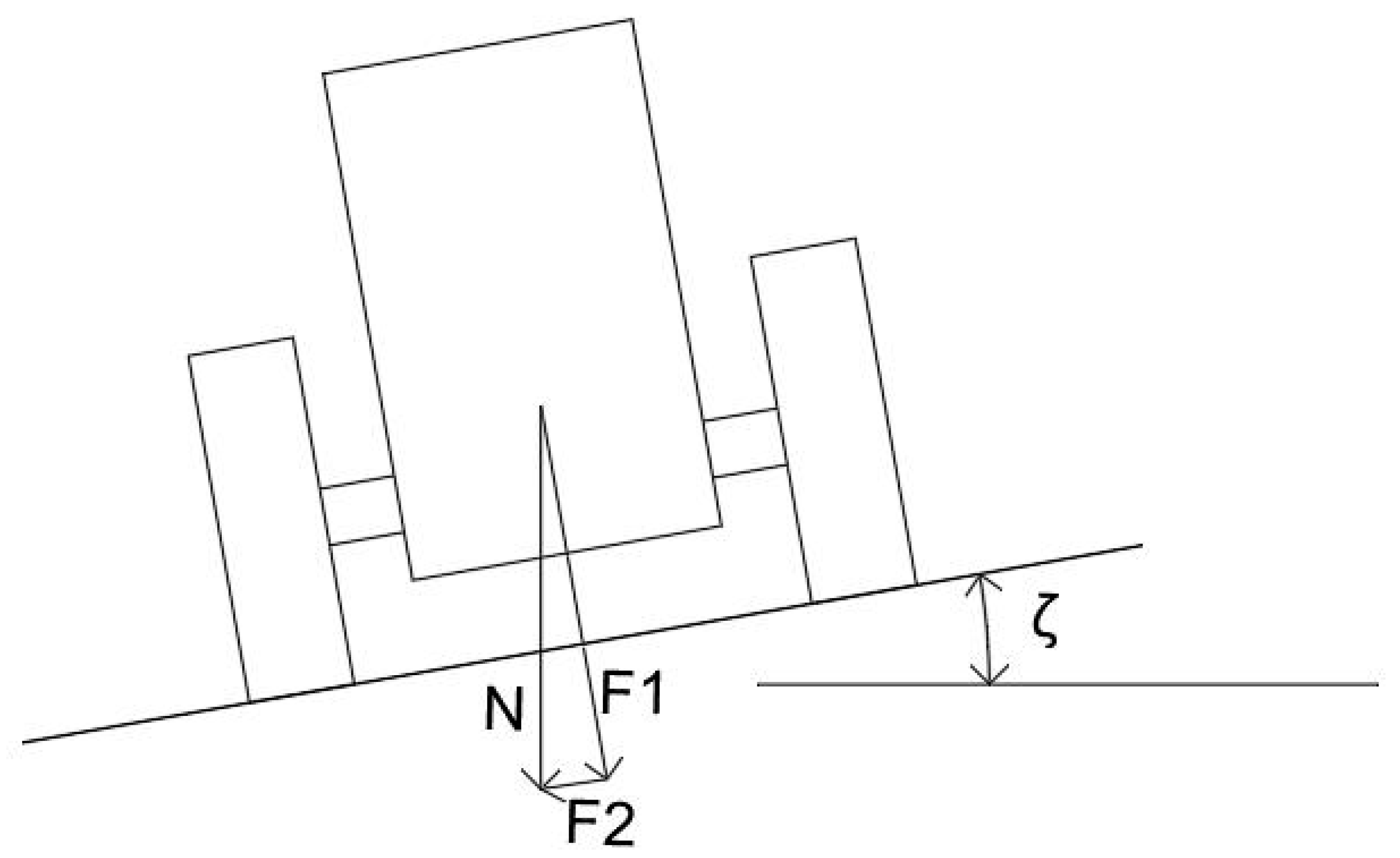
Figure 1 shows forces on a tractor while traveling on a slope.
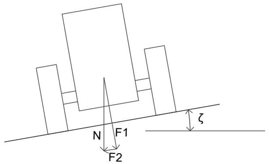
Figure 1.
Schematic diagram of forces on a tractor traveling on a slope.
As shown in Figure 1, N denotes gravitational force on the tractor, F1 denotes force on the tractor perpendicular to the ground, and F2 denotes force on the tractor parallel to the ground, i.e., lateral force. The angle made by the slope to the horizontal is denoted by . Thus, the lateral force F2 can be expressed as:
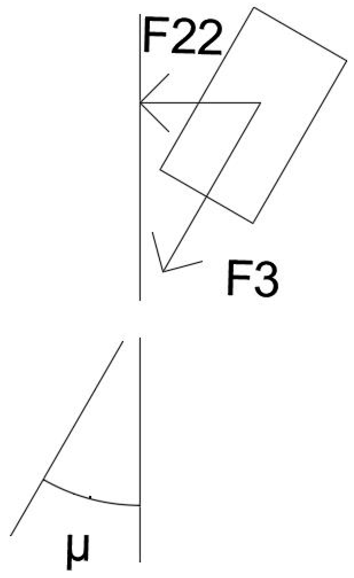
As shown in Figure 2, the steering angle of a tire is μ. F3 denotes the catch force of the tire, i.e., the force required to drive the tractor forward. F22 denotes a component of F3 perpendicular to the direction of the tractor before steering. Then, F22 can be expressed as:

Figure 2.
Mechanical relations of a tire during steering.
By utilizing the force F22 to compensate for the lateral force F2 of the tractor traveling on a slope, such that F22 = F2, it is clear that:
where K = N/F3.
It should be emphasized here that this method compensates for the steering angle of a tractor by using the force relationship of the tractor traveling on a slope to eliminate or mitigate the effects of the slope on driving performance. It is not by automatically adjusting the steering angle, which in turn induces the tractor to travel along a desired path. Nor is it an automatic steering control method that automatically adjusts a steering input to the tractor by observing a difference between the actual steering angle and the desired one.
2.2. Automatic Correction Method for Compensation Coefficients
From Equation (3), it can be seen that the compensation coefficient K is determined by the gravity force N and catching force F3 of the tractor, and by considering load changes as well as acceleration changes in the tractor in practice, we hope that the compensation coefficient K can be adjusted automatically to accurately compensate the steering angle. Moreover, in practice, it is difficult to accurately measure the gravity force N and the ground-catching force F3 on the tractor in real time. Therefore, we will introduce how to determine whether the steering angle compensator is under-compensated or over-compensated by the actual traveling paths of the tractor and its desired paths, so that the compensation coefficient K can be adjusted automatically.
Below, we describe how to automatically adjust the compensation coefficient and then obtain a compensating steering angle. Firstly, location of the tractor at the last moment is denoted as in global coordinates, and the location at the current moment is denoted as , and then its actual traveling path is roughly represented by vector , i.e., . Then we need to know the “desired path” of the tractor. Note that the “desired path” here is not a desired trajectory under trajectory tracking control as an input to a controller, but rather a route that the tractor will travel based on the initial steering angle without influence from slopes. This “desired path” can be estimated with a kinematic model. It is assumed here that the kinematic model can accurately describe the behavior of the tractor and is presented as an example. Based on the original steering angle and velocity input (denoted as and , respectively) of the tractor at the last moment, the following discretized kinematic model is then utilized [24]:
where is a discrete time variable, is the period, is a velocity input, and is a steering angle input. Based on , , and , the “desired point” can be obtained by Equation (4), and the “desired path” is denoted as . Based on the formula for the dot product of two vectors:
The angle between the real path and the “desired path” can be calculated, which is denoted as . Then, we need to know whether the real path is located on the left or right side of the “desired path” in order to determine the direction of the steering angle compensation, and we stipulate that the counterclockwise steering angle is positive and the clockwise steering angle is negative. When , the actual traveling path is on the left side of the “desired path”, so is negative; when , is positive, and the actual traveling path is on the right side of the “desired path”.
Through inertial navigation, satellite navigation, acceleration sensors, and other devices, the attitude of the tractor can be obtained, and by filtering, conversion, and fusion methods, the roll angle of the tractor can be obtained. Then, according to the previous mechanical analysis of vehicles traveling and steering on slopes, , the compensation coefficient is . Here, without distinguishing the direction of the roll angle, it is specified that the roll angle is always positive, and for ease of representation, let . Here, the gravitational force on the tractor changes as the load changes, and the ground-catching force of the tractor also changes as the vehicle acceleration changes. Therefore, in order to realize automatic adjustment of the compensating steering angle, we introduce one of the most common theoretical methods of PID controller in automatic control theory [12] to automatically adjust the value of during the tractor driving process. A simplified equation for incremental PID is as follows:
where is the discrete time variable, is the control increment, is the proportion coefficient, is the integration coefficient, is the differentiation coefficient, and is the difference between the target value and the actual output of a system. If is an angle between the actual path and the “desired path” and is the compensation coefficient , the compensation value (compensating steering angle) can be automatically adjusted. The incremental update law of the compensation coefficient is obtained as follows:
where is the proportion coefficient, is the integral coefficient, and is the differential coefficient, and those all need to be obtained according to the actual situation of the tractor and environment. The compensation coefficient is . Finally, the compensating angle is calculated as .
2.3. Steering Angle Compensation Algorithm
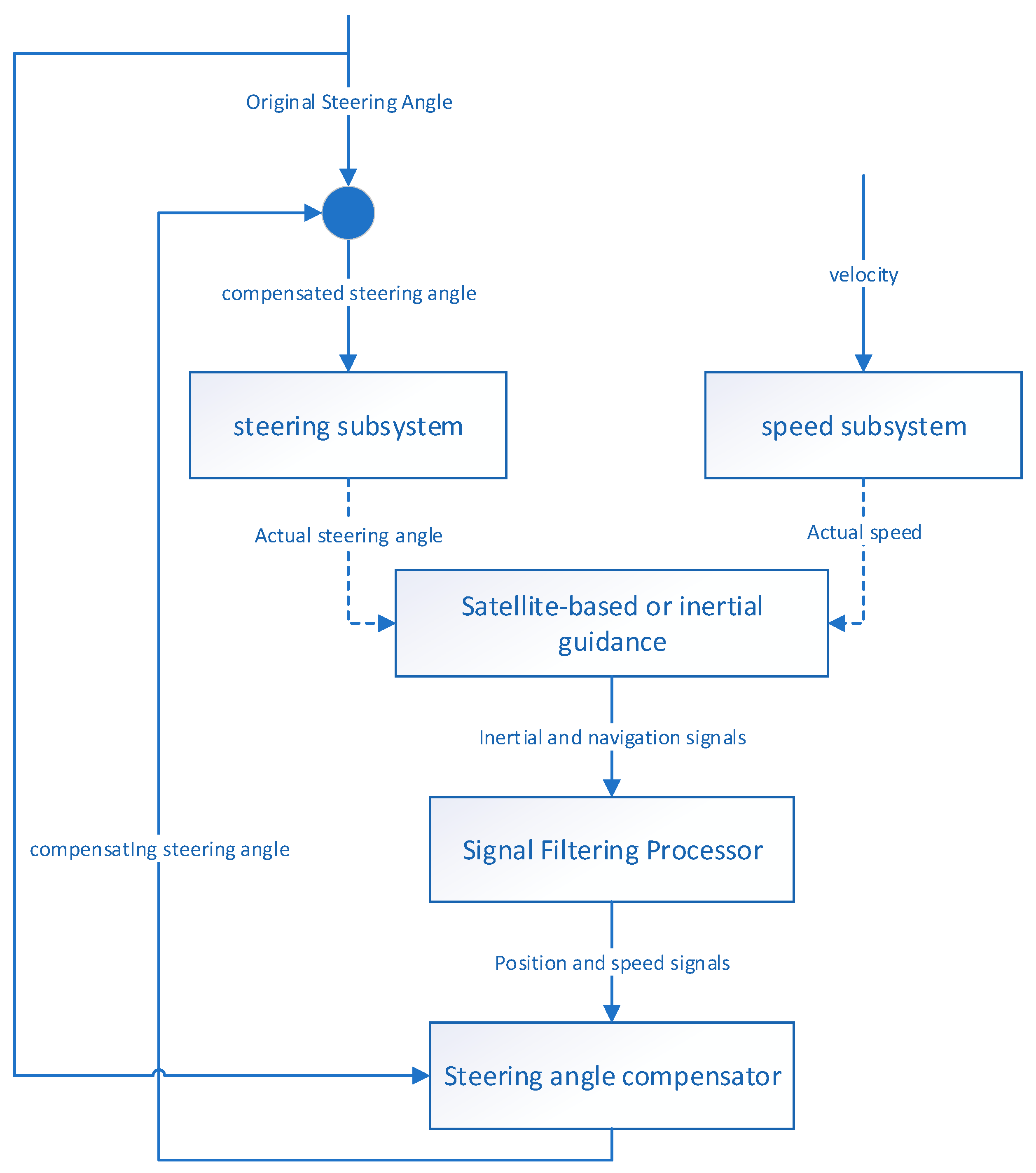
As shown in Figure 3, a schematic diagram of the principle of steering angle compensation, under the effects of compensated steering angle and velocity signals, the actual steering angle and actual velocity generated by the steering and velocity subsystems act on the tractor, respectively. In order to simplify the problem, it is assumed here that the actual steering angle is equal to the compensated steering angle signal and the actual velocity is equal to the velocity signal. The original steering angle is a steering signal given by manual steering or an automatic controller when no compensating device is added to the tractor; the compensated steering angle is obtained from the original steering control signal plus a compensating steering angle after the compensating device is added. Dotted lines in the figure indicate that actual steering angle and actual speed are not output to satellites and inertial devices in a realistic signal form, but rather signals measured by satellites and inertial devices are altered by influence on the state of the tractor. With a satellite positioning device and an inertial guidance device on the tractor, a signal filtering processor can be designed to process and estimate relevant signals to obtain the real-time position, speed, and roll angle of the tractor. A compensator based on real-time position, speed, and original steering angle signals of the tractor, using a kinematic model, according to the method introduced above to automatically calculate compensating steering angle, is used to determine the compensating steering angle plus the original steering angle to obtain a compensated steering signal and act on a steering sub-system.
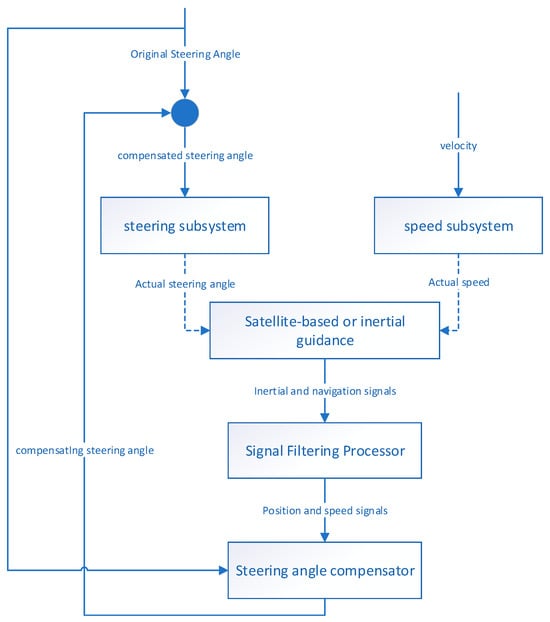
Figure 3.
Schematic diagram of the steering angle compensation.
In summary, a compensation algorithm is shown in Algorithm 1.
| Algorithm 1. Flowchart of the compensation algorithm |
| Input: proportion, integral, differential coefficient , and period . Initialized with . |
| Step 1: When , this step is skipped; otherwise, the kinematic model is used to calculate the “desired point” . Step 2: Position , original steering angle , and roll angle of the tractor are measured and obtained. Step 3: When , let the angle between the actual traveling route and the “desired route” be ; otherwise, based on position of the tractor, and the “desired point” , is calculated by Equation (5). Step 4: Based on and , the compensation coefficient is calculated by Equation (7). Step 5: Based on the roll angle and the compensation coefficient , the compensated steering angle is obtained. Step 6: The compensated steering angle is obtained and applied to the system based on summing the compensating angle with the original steering angle . Let . |
| Output: sum of the compensating angle and the original steering angle . |
Above all, it is necessary to set values for the proportional coefficient , integral coefficient , differential coefficient , and period . The initialization is carried out to make .
In the first step, when , this step is skipped; otherwise, based on the position of the last period of the tractor and the sampling period , the kinematic modeling (4) is utilized to calculate a “desired point” .
In the second step, the vehicle position , original steering angle , and roll angle are obtained by measurement.
In the third step, when , let angle , which is between the actual traveling path and the “desired path” . Otherwise, based on position of the tractor in the last period, position of it in the current period, and the “desired point” , can be calculated by utilizing the vector point multiplication Formula (5) and the judgment method of the position relationship between the actual traveling path and the “desired path”.
In the fourth step, based on and , the compensation coefficient is computed using the incremental update law (7).
In the fifth step, based on the roll angle and the compensation coefficient , the compensating steering angle is calculated using .
In the sixth step, based on the compensating steering angle , it is summed with the original steering signal to obtain a compensated steering signal and to act on the system. Let .
Finally, apply the compensated steering angle to the steering subsystem and return to the first step to repeat the calculation.
2.4. Symbols Covered in This Section and Their Meanings
Symbols covered in this section and their meanings are shown in Table 1 below:

Table 1.
Symbols and their meanings.
3. Model Predictive Control for Path Tracking of a Tractor
The steering angle compensator presented in Section 2 can be used in conjunction with a wide range of existing path tracking control methods for tractors, and this paper will take model predictive control as an example in order to illustrate in detail how this steering angle compensator can be used in conjunction with common control methods, so the model predictive controller design itself is not part of the main contribution of this paper.
This section mainly refers to Chapter 4 in book [34], which is briefly introduced as follows for the completeness of this paper. Under a fixed-coordinate system, the kinematic model of the tractor is:
where is the coordinate of the rear axle of the tractor, is the heading angle, is the turning angle, is the speed, and is the wheelbase of the tractor.
From the above equation, this is a system with inputs and states , which can be expressed in the following general form:
A given reference trajectory is also represented in the same form:
where reference values are denoted by , .
Expand Equation (10) at the reference trajectory points using a Taylor series expansion and ignore higher-order terms.
Subtracting Equation (10) from Equation (8) gives:
Further discretize Equation (11):
where, , and is the sampling time.
Transform Equation (12) as follows:
Then we get
where,
The output expression of the system can be obtained:
where,
Consider control and control increment constraints:
The objective function used is as follow:
where is the predictive horizon, is the control horizon, is the weighting coefficient, and is the relaxation factor.
4. Model Predictive Controller with Steering Angle Compensator
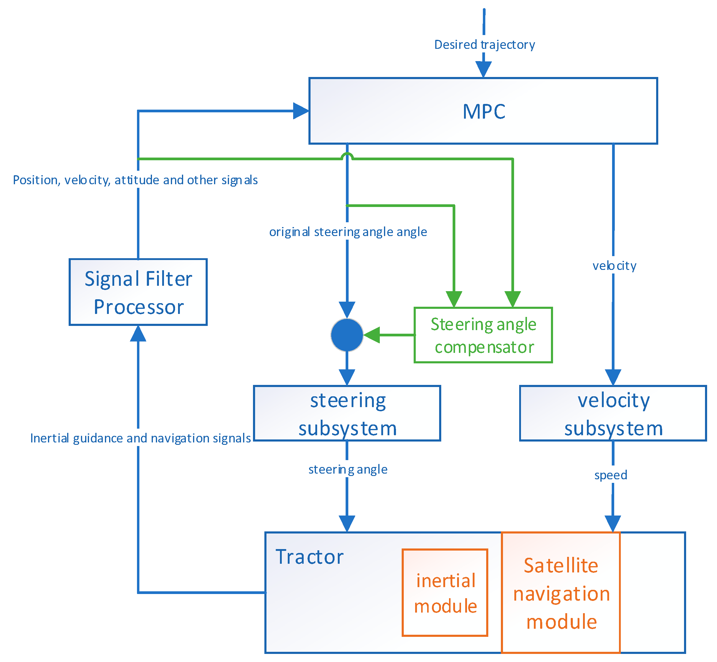
As shown in Figure 4, a schematic diagram of the steering angle compensation for path tracking control of the tractor based on a model predictive controller, the cyan marking is a compensator, and the steering angle (original steering signal) calculated by MPC is summed up with the compensating steering angle from the compensator to obtain a compensated steering angle. The compensation algorithm is the same as the one described in Section 2. It can be seen that the compensator can be independently and easily applied to an automatic path-tracking control system.
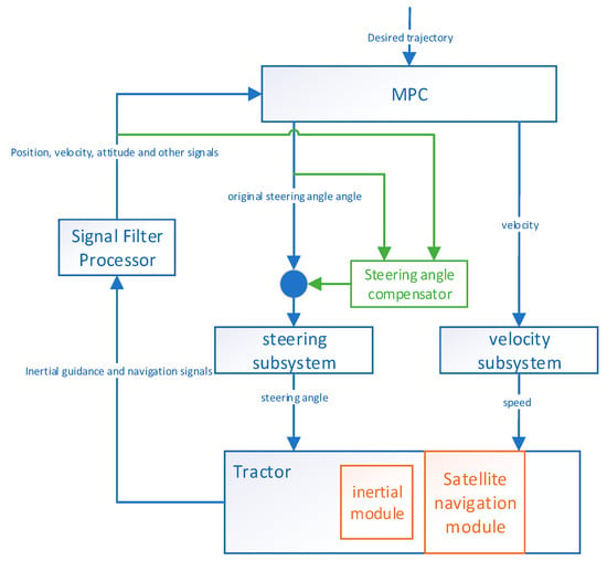
Figure 4.
Schematic of the steering angle compensation for path tracking control of the tractor.
In summary, the algorithm executed at each period when the angle compensator is embedded in a model predictive controller is shown in Algorithm 2 below:
| Algorithm 2. Flowchart of the MPC algorithm with a compensator. |
| Input: proportional, integral, and differential coefficients , real position, heading angle, speed and steering angle of the tractor roll angle reference position, heading angle, speed and steering angle series of the tractor , control and predictive horizon , weighting matrices and coefficient for objective function , upper and lower bounds for control increments and control variables as well as control period . Initialized with . |
| Step 1: Solve the optimization problem (18) to obtain the velocity control increments and the steering angle increments . And . Step 2: When , this step is skipped; otherwise, based on the previous position of the tractor as well as the velocity and steering angle outputted from MPC at the previous period , the kinematic model (4) is used to calculate the “desired point”. Step 3: When , set the angle between the actual traveling route and the “desired route” to zero, ; otherwise, let , and is calculated based on the vehicle position , , and the “desired point” using Equation (5). Step 4: Based on , and , the compensation coefficient is calculated by Equation (7) and . Step 5: Based on the roll angle and the compensation coefficient , the compensating steering angle is calculated using . Step 6: The compensating steering angle and the original steering angle are summed to obtain the compensated steering angle, which is the output and acts on the system with velocity . Let . |
| Output: compensated steering angle and velocity . |
First of all, it is necessary to set values of relevant parameters of the compensator and predictive controller, including proportional coefficient , integral coefficient , differential coefficient , period , current actual position , heading angle , speed , steering angle of the tractor, reference position, heading angle, speed and steering angle series of the tractor , control horizon , predictive horizon , weight matrices and coefficient of optimization problem (), and upper and lower bounds of constraints ), as well as initialization with .
In the first step, position (), heading angle , velocity and steering angle of the tractor in the current period are measured, and according to the reference position, heading angle, velocity, steering angle series , control horizon , predictive horizon , weighting matrices and coefficient , upper and lower bounds for control increments and control variables as well as control period , the optimization problem (18) is solved to obtain the velocity increment series and the steering angle increment series . The first element can be taken as . At the end, .
In the second step, when , this step is skipped; otherwise, based on the last position , speed , and steering angle outputted from MPC in the last period, a kinematic model (4) is utilized to compute the “desired point” .
In the third step, when k = 0, let the angle between the actual traveling path and the “desired path” be . Otherwise, based on position of the tractor in the last period, position in the current period, and the “desired point”, using the vector dot product Formula (5) and the positional relationship between the actual traveling path and the “desired path” , can be obtained.
In the fourth step, based on , and , the compensation coefficient is calculated using the incremental update law (7).
In the fifth step, based on the roll angle and the compensation coefficient , the compensating steering angle is calculated by .
In the sixth step, based on the compensating value , the compensated steering angle is obtained by summing with the steering angle , which is applied to the tractor with velocity . Let .
Finally, return to step 2 for repeated calculations.
5. Simulation Results
In this paper, experiments are conducted using simulink and carsim for joint simulation, which provides an extremely high-precision model of the tractor, while control is carried out by writing a program using the S-function module in simulink. Carsim is able to reflect the mechanics of the tractor and is recognized as a significant platform for evaluating the performances of various modeling, control, and optimization algorithms in vehicle domains.
Specific parameters of the tractor used in the simulation are shown in Table 2.

Table 2.
Tractor parameters.
The MPC parameters are configured as shown in Table 3.

Table 3.
MPC parameters.
Parameters of the PID angle compensator are configured as shown in Table 4.

Table 4.
PID parameters.
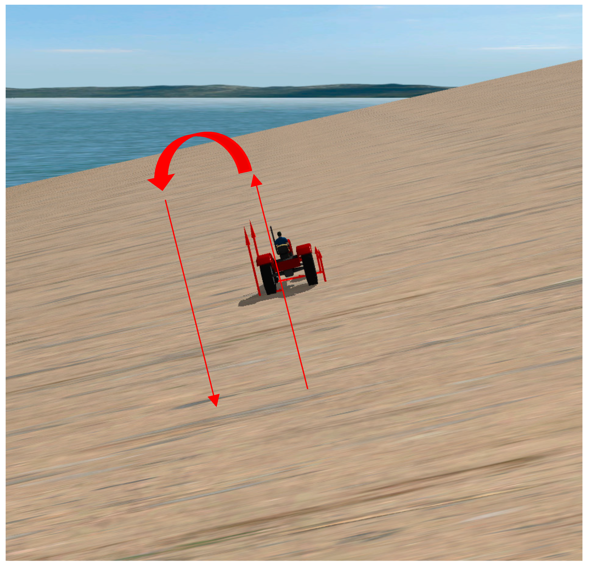
In all the simulation experiments, the tractor traveled in a sloping field, as shown in Figure 5. When the tractor was traveling in a straight line (i.e., in operation), the lateral force on the tractor was constant; when the tractor turned around, the lateral force on it would change continuously. In different groups of simulation experiments, we obtained a series of experimental results by making a single change in parameters such as slope gradient, speed during straight-line travel, and turning radius.
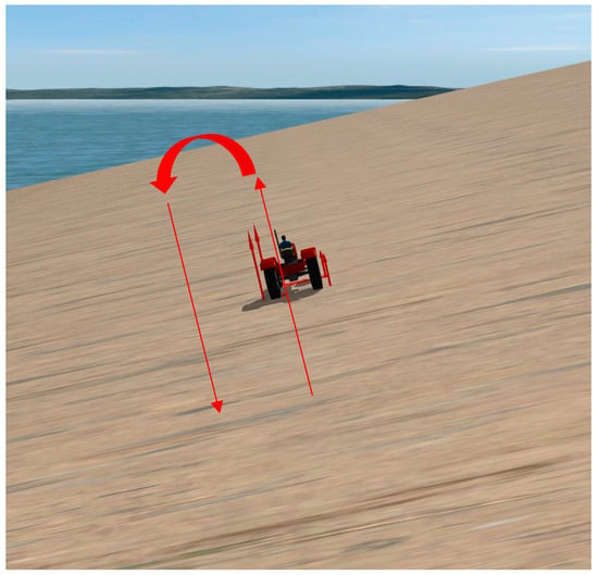
Figure 5.
Schematic representation of the topographic conditions of the slope and way of traveling in the simulation.
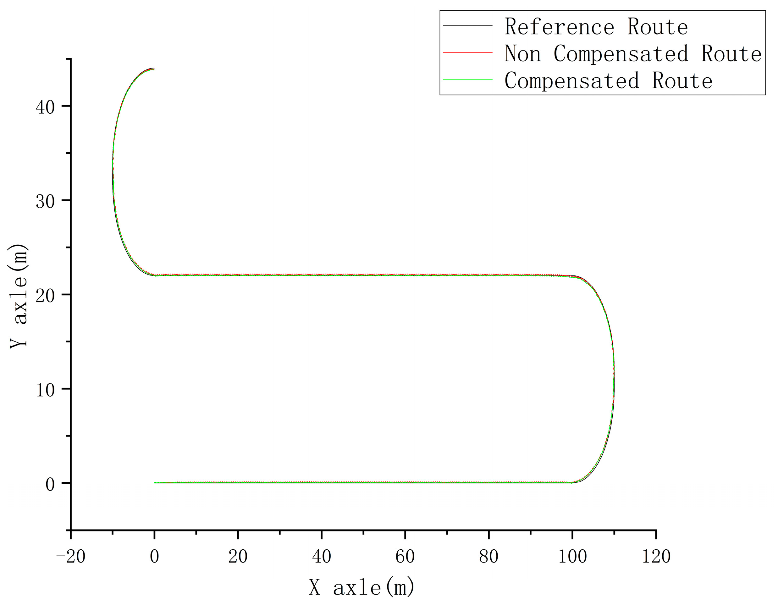
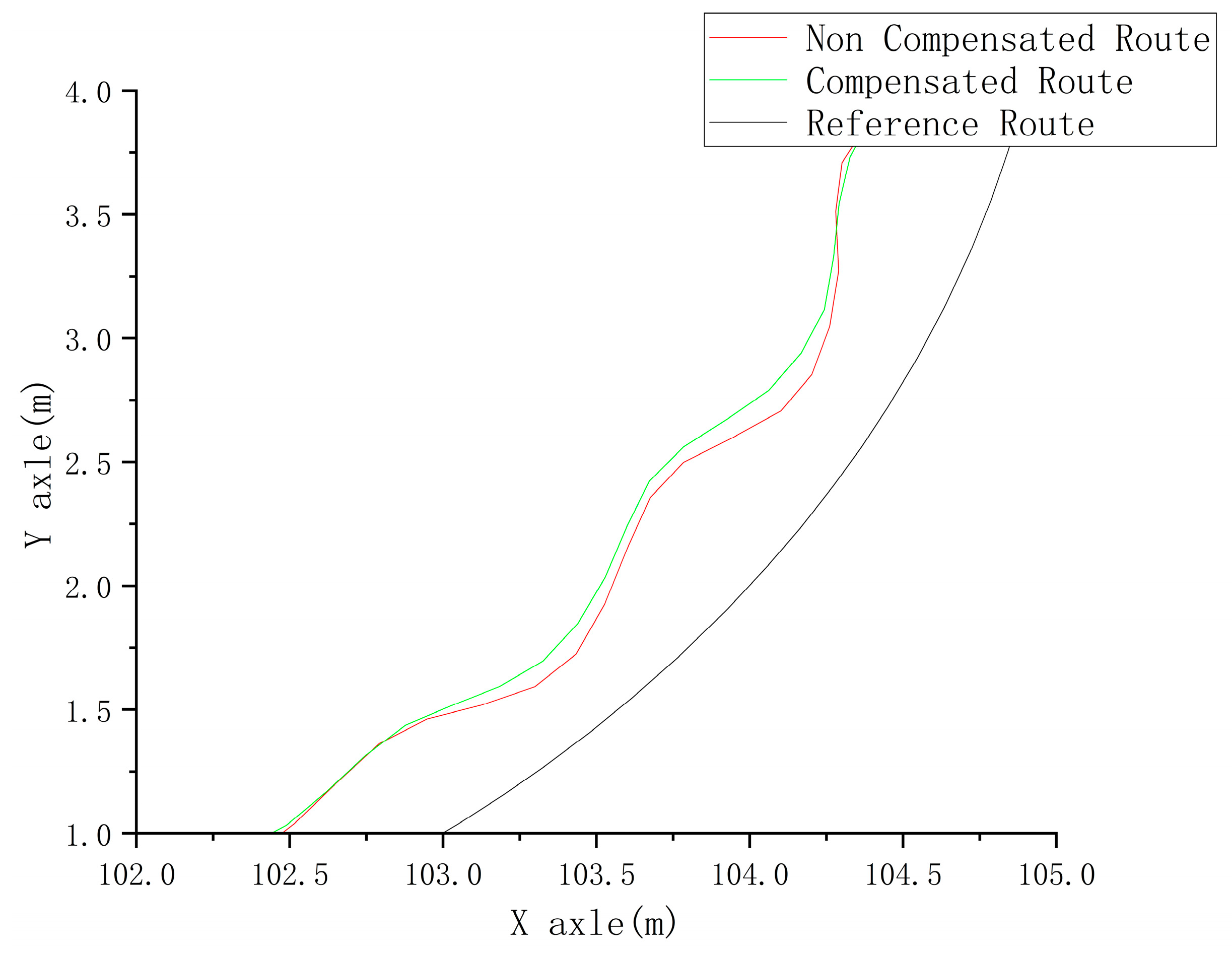
Furthermore, in order to illustrate more clearly the way the tractor travels in the simulation experiments, we take an experiment as an example to describe this in detail. The actual and reference routes of the MPC with and without an angle compensator are shown in Figure 6.
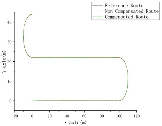
Figure 6.
(Non) compensated route vs. reference route.
Figure 6 shows the actual and reference routes of MPC with and without the addition of the angle compensator, respectively. The red curve in the figure shows the route obtained by a tractor under the control of MPC without the addition of the angle compensator, while the green curve shows a route with the addition of the compensator, and the blue one is a reference route. According to the parameter settings, the tractor starts from origin (0, 0), travels 100 m straight to (100, 0), turns one-quarter arc counterclockwise to reach (110, 10), travels 1 m straight to reach (110, 11), then turns one-quarter arc counterclockwise again to reach (100, 21). After completing the U-turn, it continues to drive straight in the opposite direction for 100 m to reach (0, 21), and then completes another clockwise U-turn, i.e., first turning clockwise through a quarter arc, then going straight for 1 m, and finally turning clockwise through another quarter arc again. Traveling in a straight line has a speed of 10 km/h, turning has a speed of 5 km/h, and making a U-turn has a radius of 10 m. From Figure 6, it can be seen that the actual path of the tractor can basically track the reference route regardless of whether an angle compensator is added or not. This result was shown in all other experiments with different parameter settings.
5.1. Simulation Results of a Tractor Traveling in a Straight Line at Different Speeds
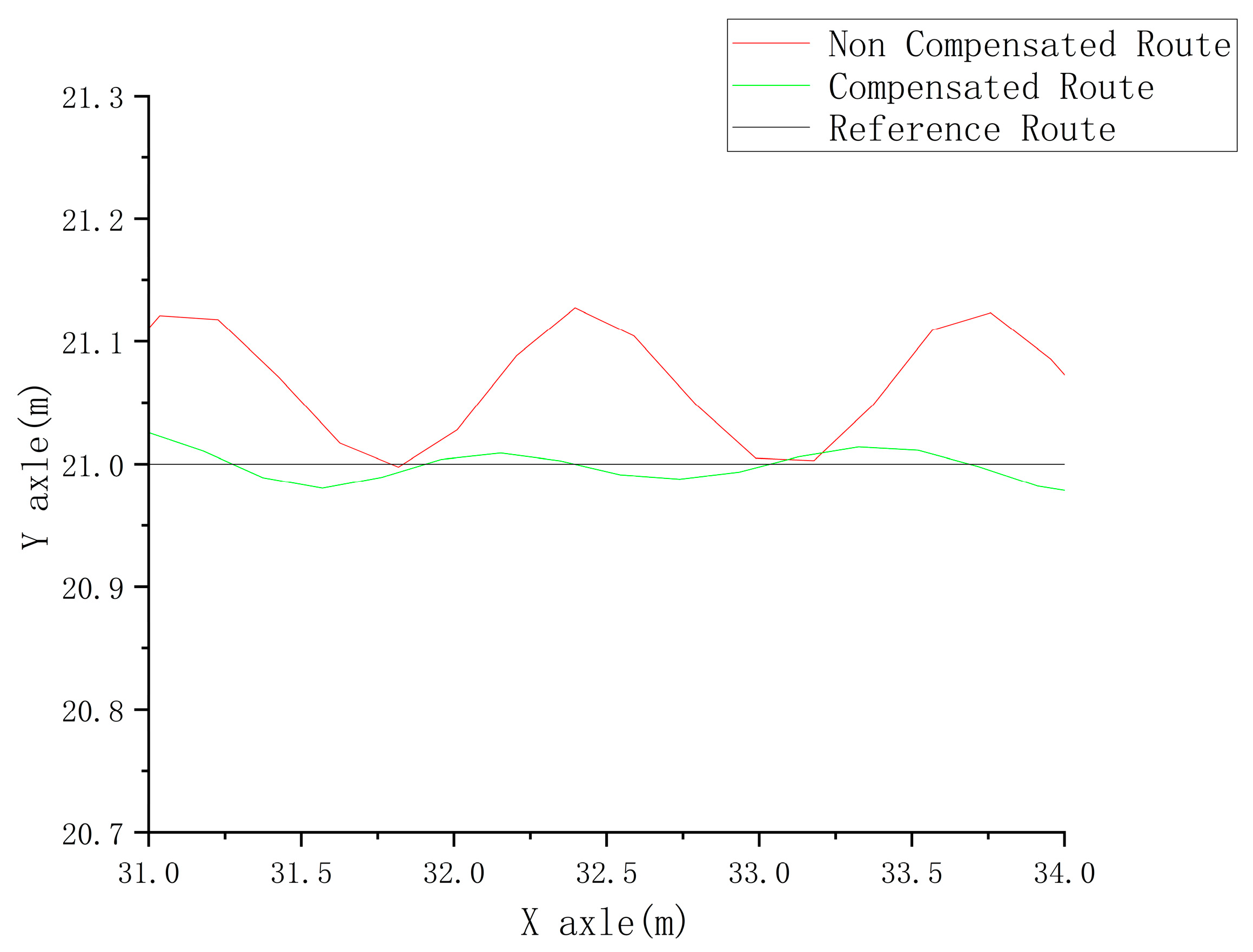
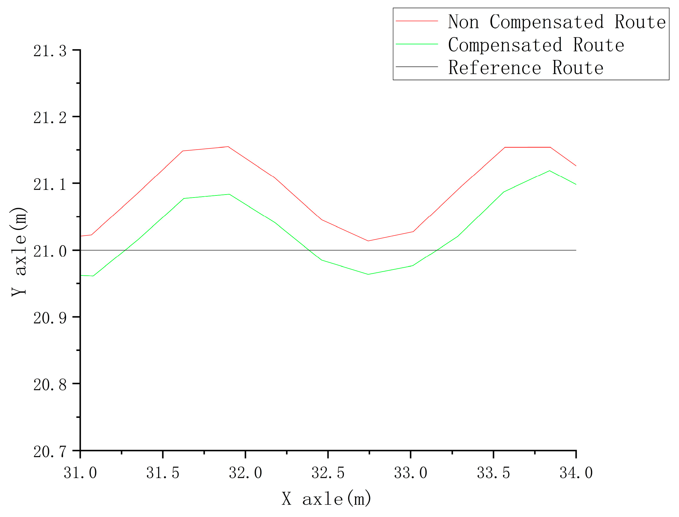
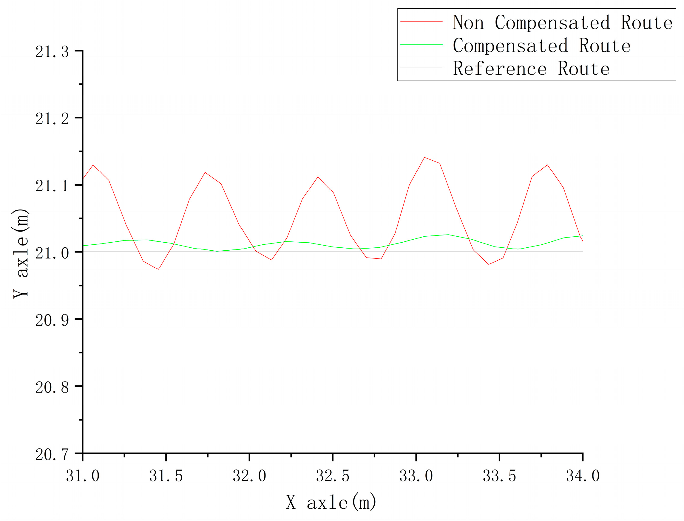
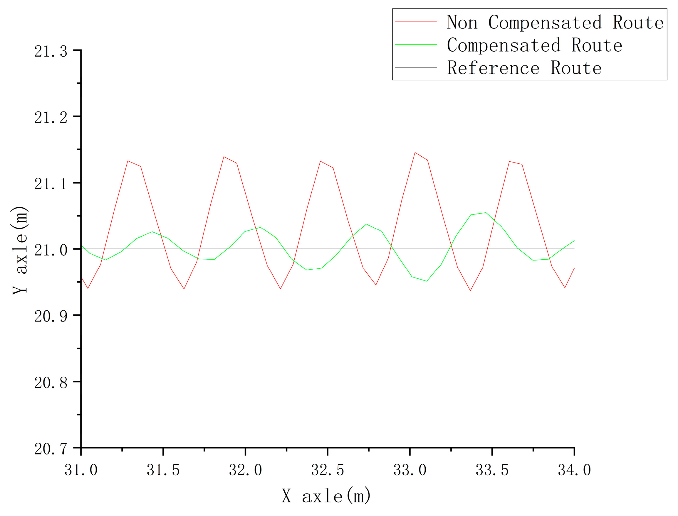
Given that the tractor’s speed in practical operating situations usually ranges between 3–7 km/h and the maximum operating speed usually does not exceed 10 km/h, we conducted four sets of experiments in simulation with speeds of 3 km/h, 5 km/h, 7 km/h, and 10 km/h. All experiments were conducted in a sloping field with a slope gradient of 0.22. The parameter settings of the MPC and compensator for different experiments in the simulation are shown in Table 5.

Table 5.
MPC and compensator parameters for different experiments.
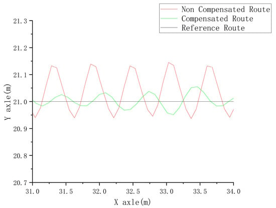
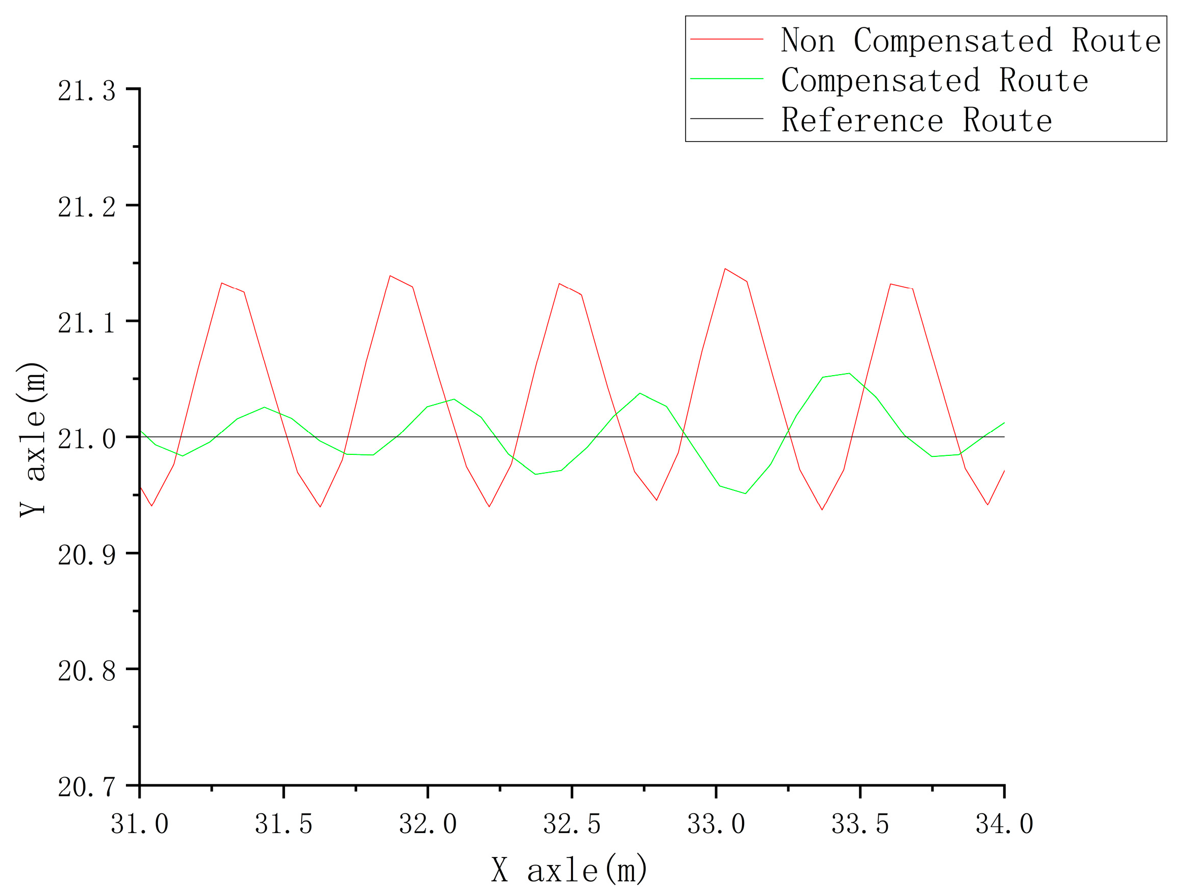
Figure 7.
(Non) compensated route vs. reference route localized (3 km/h).
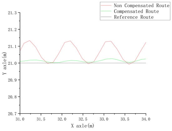
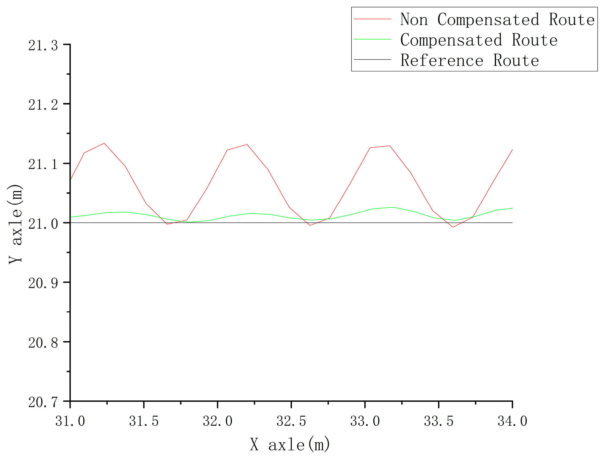
Figure 8.
(Non) compensated route vs. reference route localized (5 km/h).
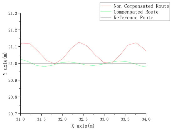
Figure 9.
(Non) compensated route vs. reference route localized (7 km/h).
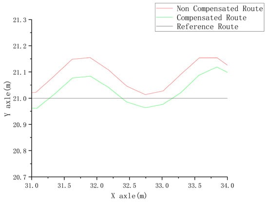
Figure 10.
(Non) compensated route vs. reference route localized (10 km/h).
From the above four simulation results, it can be intuitively seen that the steering angle compensator allows the tractor to track the reference routes better as well as make the controls smoother at different speeds. In order to better illustrate the effect of the compensator statistically, we introduce the distance between the actual traveling route and the reference route to quantify the experimental results. In the following, the average distance between the actual traveling route and the reference route , as well as the average absolute value of the distance of the actual traveling route at different simulation speeds, are given in Table 6. characterizes the degree of fluctuation of the tractor during straight-line driving, i.e., the degree of smoothness of control. The closer is to zero, the smoother the control is, and the less the tractor sways dramatically from side to side.

Table 6.
Average distance between the actual traveling route and the reference route and the average absolute value of the distance of the actual traveling route for different experiments.
From the data in Table 6, it can be seen that the inclusion of the compensator helps to reduce steady-state errors when the tractor is traveling on a slope in experiments of straight-line driving at various speeds, so that it can follow the reference route accurately. Moreover, in most cases, the compensator also makes the tractor travel more smoothly and reduces the magnitude of its side-to-side swaying.
5.2. Simulation Results of a Tractor Traveling under Different Turning Radii
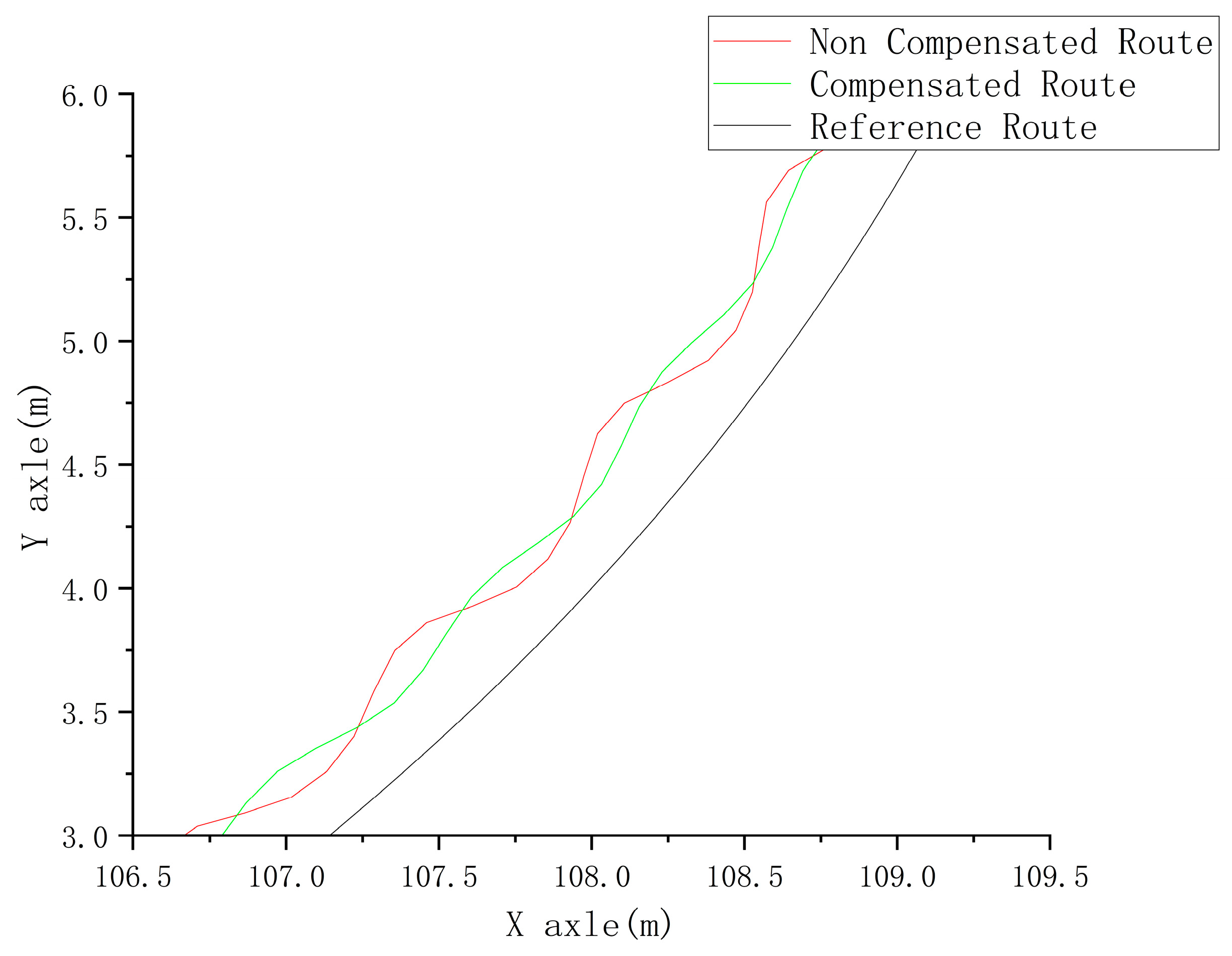
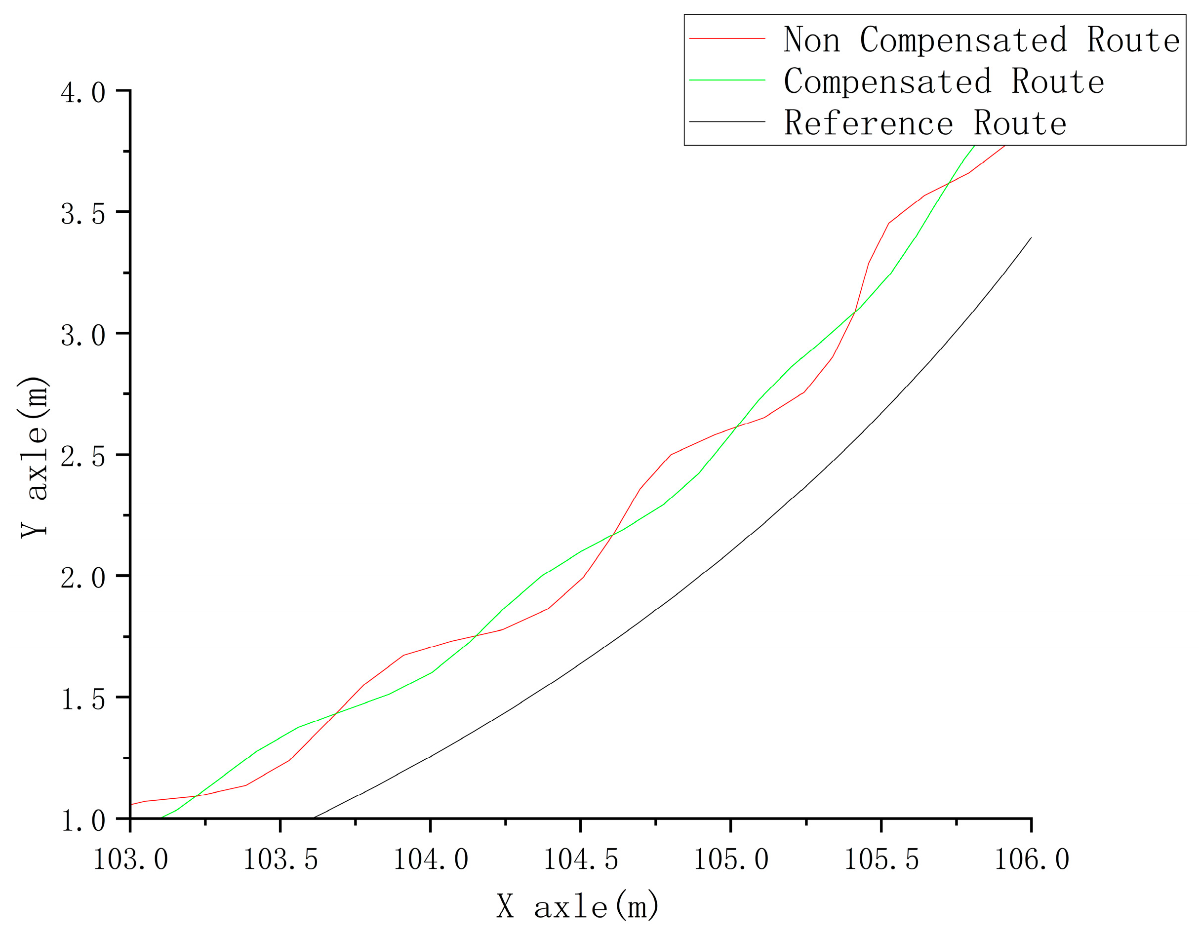
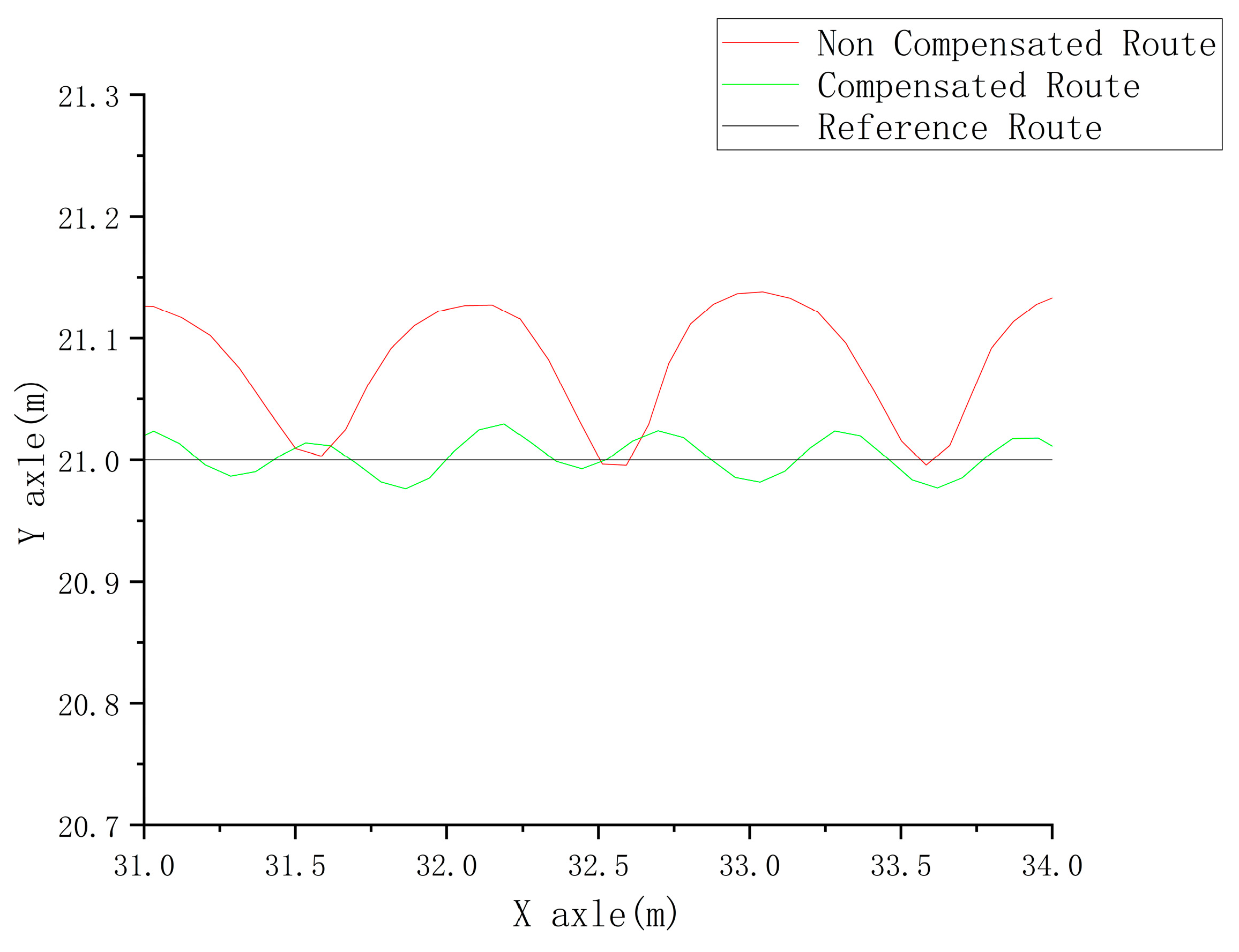
We obtained simulation results of the tractor traveling under different turning radii by setting the turning radius to 10 m, 7 m, and 5 m, respectively, in different experiments. All the experiments were carried out in a sloping field with a slope gradient of 0.22, and the speed of the tractor was 5 km/h. The parameter settings of the MPC and compensator for different experiments are shown in Table 7.

Table 7.
MPC and compensator parameters for different experiments.
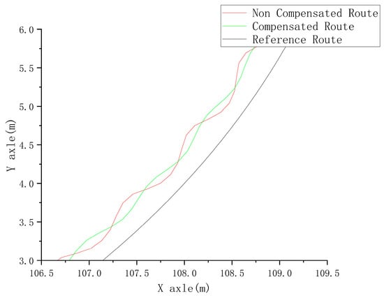
Figure 11.
(Non) compensated route vs. reference route localized (10 m).
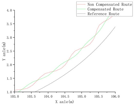
Figure 12.
(Non) compensated route vs. reference route localized (7 m).
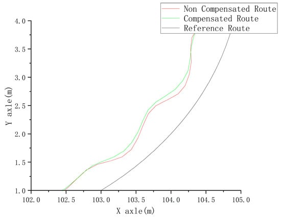
Figure 13.
(Non) compensated route vs. reference route localized (5 m).
From the above three simulation results, it can be intuitively seen that at different turning radii, the compensator does not significantly reduce the steady-state error of the path tracking control, but it makes it smoother. This is due to the fact that both the MPC and compensator use a kinematic model as a prediction model, i.e., it is assumed that the kinematic model (8) can accurately describe the motion laws of the tractor. As a matter of fact, when we use a joint simulation method between the carsim and the simulink for our experiments, the carsim provides an ultra-high-dimensional, high-precision model of the tractor. The mismatch between this model and the kinematic model becomes more and more serious when the arc of the turn is larger, i.e., when the radius is smaller. Furthermore, from the analysis in Section 2 of this paper, it can be seen that the steering angle compensator itself is also based on a model, and thus only by improving the accuracy of the adopted model can the path tracking bias be overcome more effectively.
The average distance between the actual traveling route and the reference route , as well as the average absolute value of the distance of the actual traveling route at different radii, are given in Table 8.

Table 8.
Average distance between the actual traveling route and the reference route and the average absolute value of the distance of the actual traveling route for different experiments.
5.3. Simulation Results of a Tractor Traveling under Different Slope Gradients
Relevant surveys show that the slope is below 15° on 87.5% of agricultural land [30]. Therefore, three groups were set up in our experiments with gradients of slopes of 0.11 (6.28°), 0.22 (12.42°), and 0.33 (18.27°), respectively. The speed of the tractor for all experiments was 3 km/h. The parameter settings of the MPC and compensator for different experiments are shown in Table 9.

Table 9.
MPC and compensator parameters for different experiments.
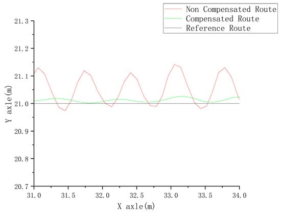
Figure 14.
(Non) compensated route vs. reference route localized (6.28°).
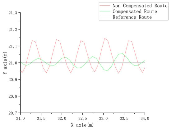
Figure 15.
(Non) compensated route vs. reference route localized (12.42°).
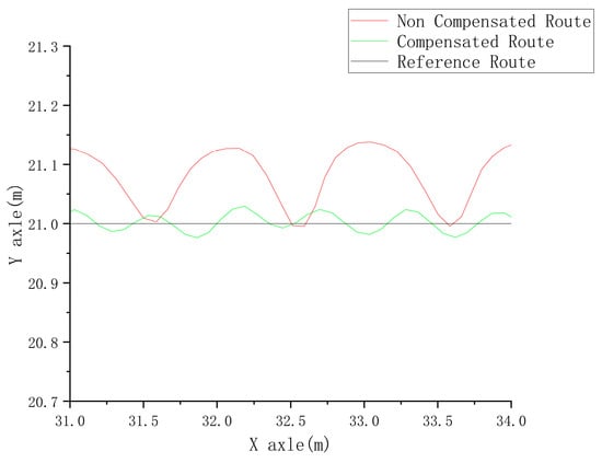
Figure 16.
(Non) compensated route vs. reference route localized (18.27°).
From the results of the above simulation experiments, it can be seen that as the gradient of the sloping land increases, the unfavorable effect on the tractor also increases. The addition of the compensator in different experiments allows the tractor to track the reference route more accurately and reduces the magnitude of left–right swaying during tracking.
The average distance between the actual traveling route and the reference route , as well as the average absolute value of the distance of the actual traveling route at different slopes, are given in Table 10.

Table 10.
Average distance between the actual traveling route and the reference route and the average absolute value of the distance of the actual traveling route for different experiments.
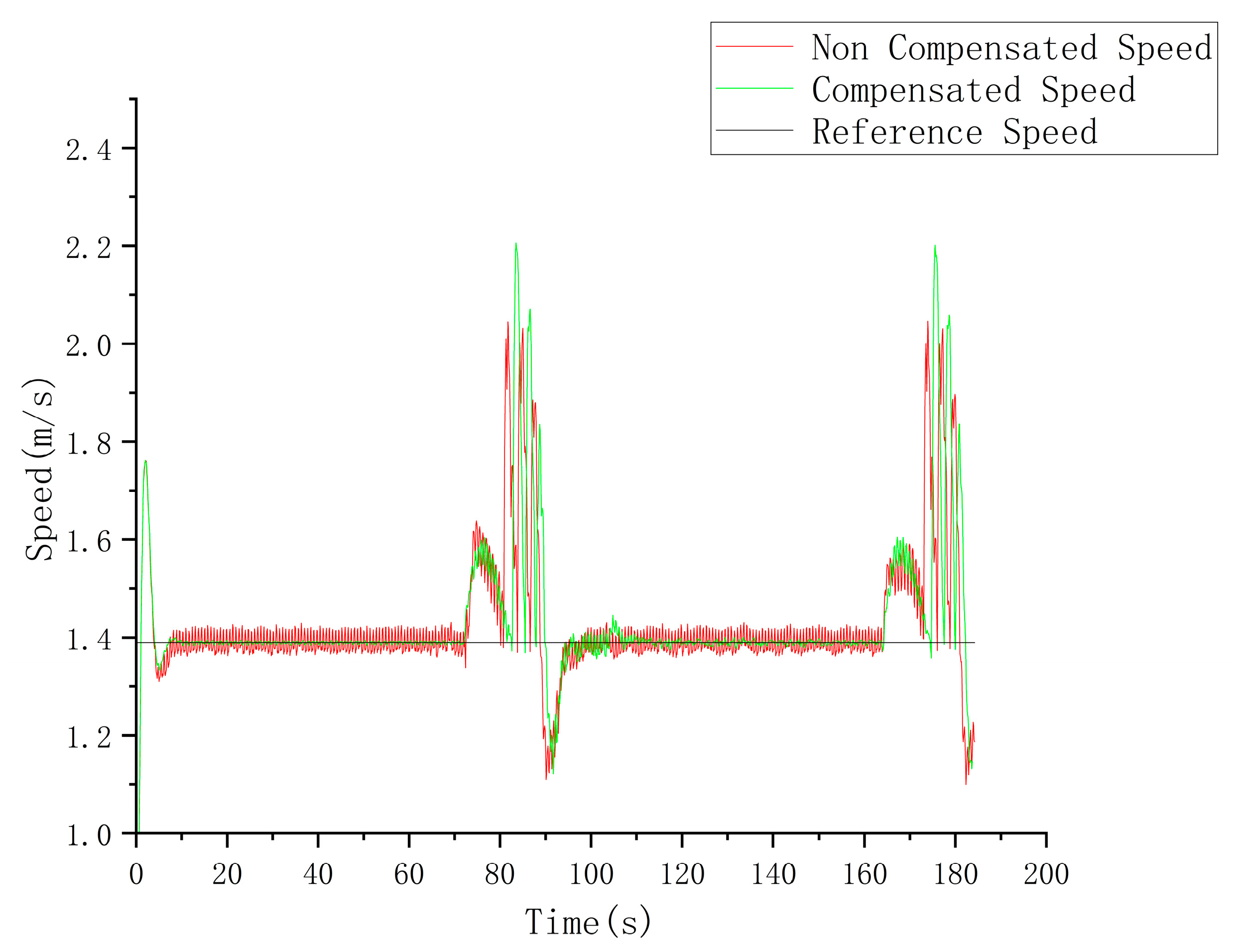
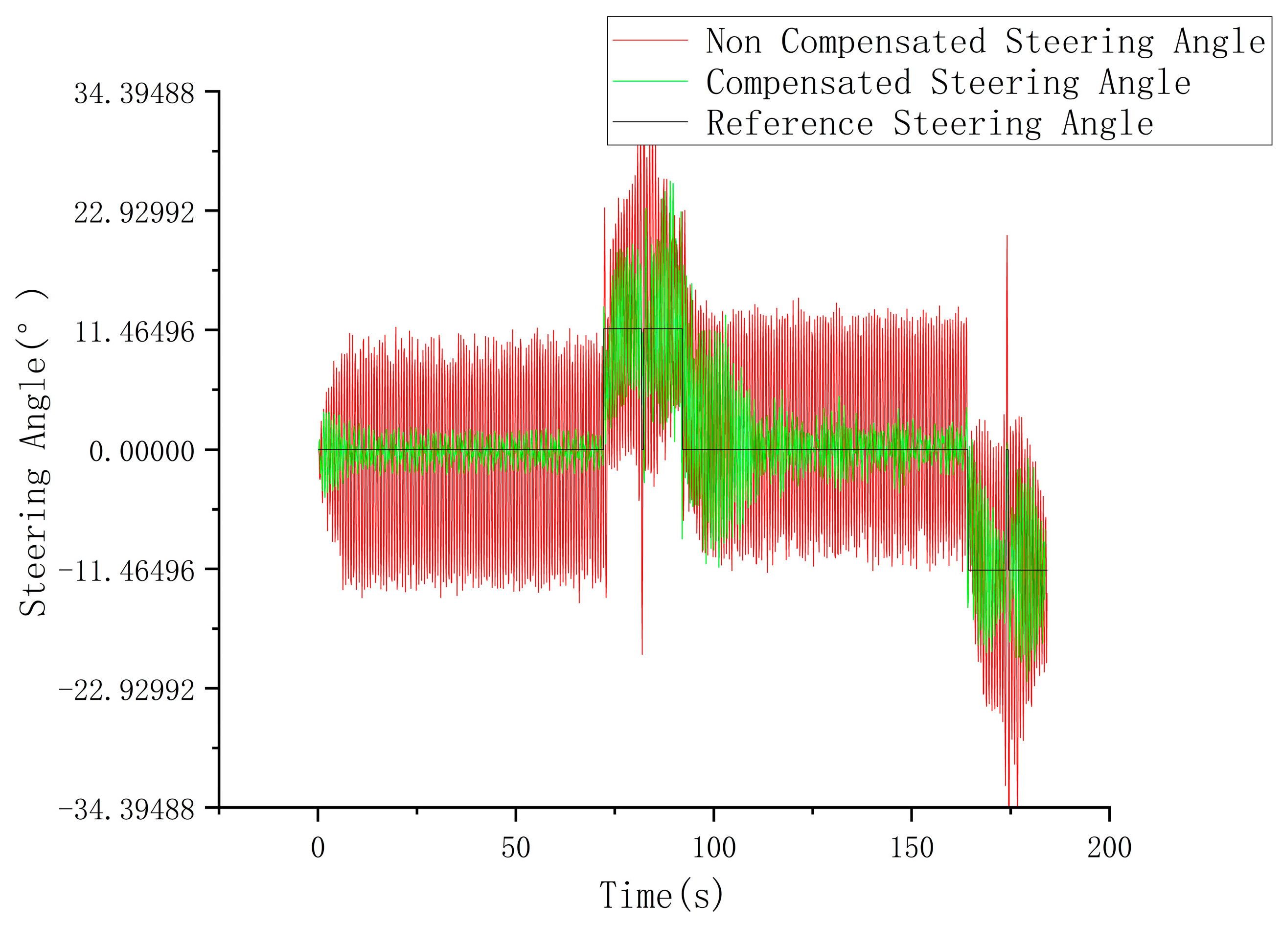
5.4. Effect of Compensator Incorporation on Speed and Steering Angle
From previous sets of experiments, it can be seen that the inclusion of the compensator can generally reduce the left–right swaying during path tracking of the tractor, and the following experimental results can lead to a similar conclusion from another aspect. In the following experiments, the speed set for straight line traveling is 5 km/h, the speed set for turning is also 5 km/h, and the turning radius is 10 m. Relevant parameters of the MPC and compensator are shown in Table 11.

Table 11.
MPC and compensator parameters for the experiment.
As shown in Figure 17, a graph of the actual speed versus the reference speed, the red curve is a speed obtained by the tractor under MPC without adding the compensation mechanism, while the green one is a speed when the compensation mechanism is added, and the black one is the reference speed. It can be seen that, in most cases, the inclusion of the compensation mechanism allows the velocity to fluctuate in a smaller range with smoother control.
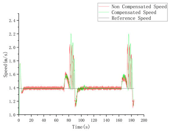
Figure 17.
Actual vs. reference speed.
As shown in Figure 18, a graph of the actual steering angle versus the reference steering angle, the red curve is a steering angle obtained when the tractor is controlled by MPC without adding the compensation mechanism, while the green one is a steering angle when the compensation mechanism is added, and the black one is a reference steering angle. It can be seen that, in most cases, the inclusion of the compensation mechanism allows the steering angle to fluctuate in a smaller range with smoother control.
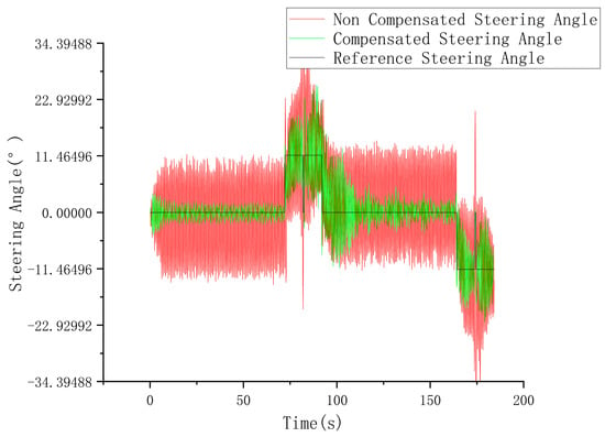
Figure 18.
Actual steering angle vs. desired steering angle.
In fact, it is an important objective to avoid frequent and large fluctuations of action mechanisms in control systems, since in general, their large fluctuations lead to an increase in the maintenance costs of associated components and even to a significant reduction in their service life.
6. Summary and Outlook
6.1. Summary
Aiming at the problem that it is more difficult to accurately track a reference route when a tractor is traveling on a slope, this paper proposes a method of compensating the lateral force on the tractor using a steering angle by analyzing the forces of the tractor when it is traveling on a slope. However, since the tractor is often affected by factors such as variable load and variable speed in practical use and it is difficult to measure mechanical parameters such as gravity force and tire-catching force of the tractor in real time, it is difficult to obtain an accurate steering compensation coefficient. For this problem, this paper proposes a method to adjust the steering compensation coefficient in real time according to the actual traveling conditions of the tractor by introducing a PID feedback mechanism so that the steering angle of the tractor can be accurately compensated in the case of changing environmental factors. Furthermore, this paper presents how this compensation mechanism can be used for a tractor system under MPC.
Finally, in order to verify the effectiveness of the compensator designed in this paper, a series of experiments were designed and simulated under different driving speeds, turning radius, and slope gradient conditions. Experimental results show that adding the compensation mechanism can reduce or even eliminate a static error in the case of straight-line driving, and it can keep speed and steering angle of the tractor in a smaller fluctuation range when driving, i.e., a smoother control. The results show that this method can effectively reduce the adverse effects of tractors traveling on slopes.
6.2. Outlook
In this paper, we have designed a steering angle compensator and used model predictive control as an example of how this compensator can be used for the path tracking control task of a tractor. In fact, as can be seen from the contents of this paper, the implementation of the compensator does not depend on the model predictive controller; in other words, the compensator can be used in a wide range of various other forms of controllers, and we would like to see a wide range of research on the combination of this compensator with other controllers in the future.
On the other hand, we also believe that the application of this compensator is not limited to tractors. The compensator presented in this paper uses a simple kinematic model, and by adapting it to other types of vehicle models, it should be applicable to special vehicles such as tracked vehicles, four-wheel steered vehicles, tractors with trailers, and others.
Author Contributions
Conceptualization, J.O. and L.X.; methodology, J.O. and L.X.; software, J.O.; validation, J.O. and L.X.; formal analysis, J.O. and L.X.; investigation, J.O. and L.X.; resources, L.X.; data curation, J.O.; writing—original draft preparation, J.O.; writing—review and editing, L.X.; visualization, J.O.; supervision, L.X.; project administration, L.X.; funding acquisition, Q.F., R.T., and J.D. All authors have read and agreed to the published version of the manuscript.
Funding
This work was supported by the Ministry of Education—China Mobile Research Fund major project (MCM2020—J-2).
Institutional Review Board Statement
Not applicable.
Data Availability Statement
Data are contained within the article.
Conflicts of Interest
The authors declare no conflict of interest.
References
- Wang, H.; Wang, G.; Luo, X.; Zhang, Z.; Gao, Y.; He, J.; Yue, B. Path tracking control method of agricultural machine navigation based on aiming pursuit model. Trans. Chin. Soc. Agric. Eng. 2019, 35, 11–19. [Google Scholar]
- Han, X.Z.; Kim, H.-J.; Moon, H.-C.; Kang, Y.-S.; Kim, J.-H.; Kim, Y.-J. Development of path generation algorithms for Korean auto-guidance tillage tractor. In Proceedings of the American Society of Agricultural and Biological Engineers Annual International Meeting, Dallas, TX, USA, 29 July–1 August 2012; pp. 4723–4732. [Google Scholar]
- Han, J.-H.; Park, C.-H.; Kwon, J.H.; Lee, J.; Kim, T.S.; Jang, Y.Y. Performance Evaluation of Autonomous Driving Control Algorithm for a Crawler-Type Agricultural Vehicle Based on Low-Cost Multi-Sensor Fusion Positioning. Appl. Sci. 2020, 10, 4667. [Google Scholar] [CrossRef]
- Han, X.Z.; Kim, H.J.; Kim, J.Y.; Yi, S.Y.; Moon, H.C.; Kim, J.H.; Kim, Y.J. Path-tracking simulation and field tests for an auto-guidance tillage tractor for a paddy field. Comput. Electron. Agric. 2015, 112, 161–171. [Google Scholar] [CrossRef]
- Li, G.; Wang, Y.; Guo, L.; Tong, J.; He, Y. Improved Pure Pursuit Algorithm for Rice Transplanter Path Tracking. Trans. Chin. Soc. Agric. Mach. 2018, 49, 21–26. [Google Scholar]
- Yao, L.; Pitla Santosh, K.; Yang, Z.; Xia, P.; Zhao, C. Path tracking of mobile platform in agricultural facilities based on ultra wideband wireless positioning. Trans. Chin. Soc. Agric. Eng. 2019, 35, 17–24. [Google Scholar]
- Zhang, W.; Ai, C.-S.; Zhang, Y.-Z.; Li, W.-X. Intelligent path tracking control for plant protection robot based on fuzzy PD. In Proceedings of the 2nd International Conference on Advanced Robotics and Mechatronics (ICARM), Hefei, China, 27–31August 2017; pp. 88–93. [Google Scholar]
- Taka, R.; Barawid, O.; Ish, K.; Noguch, N. Development of Crawler-Type Robot Tractor based on GPS and IMU. IFAC Proc. Vol. 2010, 43, 151–156. [Google Scholar] [CrossRef]
- Arvanitis, K.G.; Pasgianos, G.D.; Kalogeropoulos, G. Controller design for automatic guidance of agricultural vehicles at high field speeds. In Proceedings of the 15th Mediterranean Conference on Control and Automation, Athens, Greece, 27–29 June 2007; p. 1403. [Google Scholar]
- English, A.; Ross, P.; Ball, D.; Upcroft, B.; Corke, P. Learning Crop Models for Vision-Based Guidance of Agricultural Robots. In Proceedings of the IEEE/RSJ International Conference on Intelligent Robots and Systems (IROS), Hamburg, Germany, 28 September–2 October 2015; pp. 1158–1163. [Google Scholar]
- Hu, J.; Li, T. Cascaded navigation control for agricultural vehicles tracking straight paths. Int. J. Agric. Biol. Eng. 2014, 7, 36–44. [Google Scholar]
- Zhang, M.; Lu, X.; Tao, J.; Yin, W.; Feng, X. Design and Experiment of Automatic Guidance Control System in Agricultural Vehicle. Trans. Chin. Soc. Agric. Mach. 2016, 47, 42–47. [Google Scholar]
- Liu, Z.; Chen, Y.; Xi, Y.; Liu, G.; Zhang, M.; Liu, J. Machine Vision Based Path Tracking for Agricultural Vehicles. J. Agric. Mach. 2009, 40, 18–22. [Google Scholar]
- Ding, Y.; Zhan, P.; Zhou, Y.; Yang, J.; Zhang, W.; Zhu, K. Design and experiment of motion controller for information collection platform in field with Beidou positioning. Trans. Chin. Soc. Agric. Eng. 2017, 33, 178–185. [Google Scholar]
- Jeon, C.W.; Kim, H.-J.; Han, X.Z.; Kim, J.-H. Fuzzy logic-based steering controller for an autonomous head—Feed combine harvester. In Proceedings of the 2017 ASABE Annual International Meeting, Spokane, WA, USA, 16–19 July 2017. [Google Scholar]
- Meng, Q.; Qiu, R.; He, J.; Zhang, M.; Ma, X.; Liu, G. Development of agricultural implement system based on machine vision and fuzzy control. Comput. Electron. Agric. 2015, 112, 128–138. [Google Scholar] [CrossRef]
- Wang, F.J.; Hang, B. Path Tracking Control For a Four Wheel Differentially Steered Vision Robot. In Proceedings of the 11th International Conference on Electrical Machines and Systems, Huazhong Univ Sci & Technol, Wuhan, China, 17–20 October 2008; pp. 1608–1611. [Google Scholar]
- Wei, L.; Zhang, X.; Jia, Q.; Liu, Y. Automatic Navigation System Research for PZ60 Rice Planter. In Proceedings of the 8th IFIP WG 5.14 International Conference (CCTA), Beijing, China, 16–19 September 2014; pp. 653–661. [Google Scholar]
- Xie, Y.; Yin, J.; Yu, C.; He, K.; Hu, X.; Li, R. Obstacle Avoidance Navigation Algorithm and Analog Experiment for Wheeled AGV Running along Vineyard Ridge Road. Trans. Chin. Soc. Agric. Mach. 2018, 49, 13–22. [Google Scholar]
- Zhang, T.; Li, H.; Chen, D.; Huang, P.; Zhuang, X. Agricultural Vehicle Path Tracking Navigation System Based on Information Fusion of Multi-source Sensor. Trans. Chin. Soc. Agric. Mach. 2015, 46, 37–42. [Google Scholar]
- Zhou, J.; Cao, M.g.; Zhang, M.; Li, S. Remote Monitoring and Automatic Navigation System for Agricultural Vehicles Based on WLAN. In Proceedings of the 4th International Conference on Wireless Communications, Networking and Mobile Computing, Dalian, China, 12–17 October 2008; IEEE: Piscataway, NJ, USA; p. 2991. [Google Scholar]
- Zhou, J.; Wang, X.; Wang, X.; Liu, G.; Li, S. Autonomous Navigation System based on GPS for Agricultural Vehicles. In Proceedings of the International Forum on Mechanical and Material Engineering (IFMME 2013), Guangzhou, China, 13–14 June 2013; p. 1404. [Google Scholar]
- Zhou, J.; Zhang, M.; Cao, M.g.; Li, S.; Liu, B. Automatic navigation system for electric power vehicles with EPS. In Proceedings of the 2008 IEEE Vehicle Power and Propulsion Conference (VPPC), Piscataway, NJ, USA, 3–5 September 2008. [Google Scholar]
- Liu, Z.; Zhang, W.; Lu, Z.; Zheng, W.; Mu, G.; Cheng, X. Design on Trajectory Tracking Controller of Agricultural Vehicles under Disturbances. Trans. Chin. Soc. Agric. Mach. 2018, 49, 378–386. [Google Scholar]
- Mitsuhashi, T.; Chida, Y.; Tanemura, M. Autonomous Travel of Lettuce Harvester using Model Predictive Control. In Proceedings of the 6th International-Federation-of-Automatic-Control (IFAC) Conference on Sensing, Control and Automation Technologies for Agriculture (AGRICONTROL), Sydney, Australia, 4–6 December 2019; pp. 155–160. [Google Scholar]
- Peilin, X.; Yuan, W.; Guodong, Y.; Shuaipeng, L.; Yunyi, S. Path Tracking of Orchard Tractor Based on Linear Time-varying Model Predictive Control. In Proceedings of the 2019 Chinese Control And Decision Conference (CCDC), Piscataway, NJ, USA, 3–5 June 2019. [Google Scholar]
- Xu, G.; Chen, M.; He, X.; Pang, H.; Miao, H.; Cui, P.; Wang, W.; Diao, P. Path following control of tractor with an electro-hydraulic coupling steering system: Layered multi-loop robust control architecture. Biosyst. Eng. 2021, 209, 282–299. [Google Scholar] [CrossRef]
- Yao, Z.; Liu, G.; Zhang, D.; Shen, Y.; Wang, Z. Path Tracking Control for Four-Wheel-Independent-Driven Agricultural High Clearance Sprayer with New Front-Rear-Dual-Steering-Axle. In Proceedings of the 2020 Chinese Automation Congress, Shanghai, China, 6–8 November 2020. [Google Scholar]
- Yiheng, L.; Guodong, Y.; Qingfeng, L.; Li, W. Cross-line-Turn Path Tracking of Intelligent Agricultural Vehicle Based on MPC in Standard Orchard. In Proceedings of the 2018 Chinese Control And Decision Conference (CCDC), Piscataway, NJ, USA, 9–11 June 2018. [Google Scholar]
- Sun, J.; Liu, Z.; Yang, F.; Sun, Q.; Liu, Q.; Luo, P. A Review of Research on Agricultural Equipment and Key Technologies for Slope Operations in Hilly Mountainous Areas. J. Agric. Mach. 2023, 54, 1–18. [Google Scholar]
- Kraus, T.; Ferreau, H.J.; Kayacan, E.; Ramon, H.; De Baerdemaeker, J.; Diehl, M.; Saeys, W. Moving horizon estimation and nonlinear model predictive control for autonomous agricultural vehicles. Comput. Electron. Agric. 2013, 98, 25–33. [Google Scholar] [CrossRef]
- Backman, J.; Oksanen, T.; Visala, A. Nonlinear model predictive trajectory control in tractor-trailer system for parallel guidance in agricultural field operations. IFAC Proc. Vol. 2010, 43, 133–138. [Google Scholar] [CrossRef]
- Hill, A.; Laneurit, J.; Lenain, R.; Lucet, E. Online gain setting method for path tracking using CMA-ES: Application to off-road mobile robot control. In Proceedings of the IEEE/RSJ International Conference on Intelligent Robots and Systems (IROS), Electr Network, 24 October–24 January 2020; IEEE: Piscataway, NJ, USA; pp. 7697–7702. [Google Scholar]
- Gong, J.; Xu, Y.J.W. Trajectory tracking control for a given trajectory. In Model Predictive Control for Driverless Vehicles; Beijing Institute of Technology Press: Beijing, China, 2014; pp. 74–81. [Google Scholar]
Disclaimer/Publisher’s Note: The statements, opinions and data contained in all publications are solely those of the individual author(s) and contributor(s) and not of MDPI and/or the editor(s). MDPI and/or the editor(s) disclaim responsibility for any injury to people or property resulting from any ideas, methods, instructions or products referred to in the content. |
© 2023 by the authors. Licensee MDPI, Basel, Switzerland. This article is an open access article distributed under the terms and conditions of the Creative Commons Attribution (CC BY) license (https://creativecommons.org/licenses/by/4.0/).

