Article

Variability in Estimating Crop Model Genotypic Parameters: The Impact of Different Sampling Methods and Sizes

1
State Key Laboratory of Efficient Utilization of Arid and Semi-arid Arable Land in Northern China, The Institute of Agricultural Resources and Regional Planning, Chinese Academy of Agricultural Sciences, Beijing 100081, China
2
Collaborative Innovation Center on Forecast and Evaluation of Meteorological Disasters, Nanjing University of Information Science & Technology, Nanjing 210044, China
3
School of Environmental Science and Engineering, Tiangong University, Tianjin 300387, China
4
Agricultural Information Institute of Chinese Academy of Agricultural Sciences, Beijing 100081, China
*
Author to whom correspondence should be addressed.
Agriculture 2023, 13(12), 2207; https://doi.org/10.3390/agriculture13122207
Submission received: 31 October 2023 / Revised: 24 November 2023 / Accepted: 27 November 2023 / Published: 28 November 2023
(This article belongs to the Section Crop Genetics, Genomics and Breeding)

Abstract

:
Generic parameter calibration for crop growth models is a very important step in model use. However, studies of the effect of sample size and sampling methods on the calibration and validation of genotypic parameters have seldom been conducted. Scientists commonly apply the hold-out (HO) method, by default, to deal with samples for calibration and validation in the practice of model use. In this paper, we applied the hold-out, cross-validation (CA), and bootstrapping (BS) methods with different sample sizes to analyze the influence of sampling methods and sample size on the final calibration results of genotypic parameters. The results showed that, (1) overall, CA and BS performed better than HO at most observation stations. However, there was great variability in the calibration and validation results obtained from the three methods. (2) Because of data quality differences, we could not conclude that the more samples there were, the greater the validation accuracy of the three methods. (3) The CV of the genotypic parameter values for the three methods and sample sizes varied greatly. Thus, when genotypic parameter calibration is performed, both sampling methods and sample size should be considered.

1. Introduction

Since crop growth models have the unique advantage of providing in-depth information regarding the interaction between crop genotypic traits and environmental variables, management practices, such as DSSAT, APSIM, and WOFOST, have been widely applied [1,2,3,4]. Crop growth models are expressed by mathematical equations and functions, which represent the physiological and physical processes of the crop life cycle [5]. Because not every aspect of cropping systems can be effectively modeled, various sources of uncertainty exist in the crop-modeling process [6]. Notably, observation, model, and prediction uncertainties have been summarized to perform corresponding analyses [7]. Model inputs, model structure, and model parameters have been defined as the three major sources of model uncertainties [7,8,9]. Decomposing and quantifying sources of uncertainty not only enhances the scientific validity and practicality of crop models but also aids in making more effective decisions in agricultural production and resource management [10].
Parameter uncertainty arises from variability in model parameter values. This can stem from the data used for calibration, the limited amount of available data, or the calibration process itself. [11]. The parameters of a crop growth model can be categorized into genotypic parameters, soil parameters, management practice parameters, and other parameters, of which genotypic parameters are characterized by comparatively strong uncertainty [12,13]. Uncertainty in genotypic parameters is mainly derived from low-quality calibration data, limited calibration samples, and inappropriate calibration methods [10]. Observation and input uncertainty, which is usually caused by using indirect observation data, in the calibration process of genotypic parameters has a significantly negative impact on the accuracy of the final output [14,15]. The calibration methods for estimating genotypic parameters and the customized application of a method by users also influence eventual results. Some articles have estimated parameters by using trial and error [16,17], whereas others have used different approaches for calibration, such as GLUE [18,19,20], EFAST [21,22], and Bayesian approaches, including the Markov chain Monte Carlo (MCMC) algorithm, the MCMC method based on the Adaptive Metropolis algorithm (MCMC-AM) algorithm [22,23,24,25], etc., resulting in different ways of estimating parameter uncertainty. In addition, the genetic algorithm (GA) [26], the shuffled complex evolution method (SCE-UA) developed by the University of Arizona [5,27], particle swarm optimization [28,29], simplex algorithm (SA) [30], maximum likelihood solution (MLS) [31], Powell’s conjugate direction method (PCD) [32], the annealing algorithm (AA) [33], and the unconstrained Levenberg–Marquardt algorithm (ULM) [34] have also been applied to estimate the genotypic parameters of crop growth models. In addition, in the calibration process for genotypic parameters, the initial value range of parameters, the number of algorithm iterations, and the selection of the objective function impact the quantification of uncertainty [35]. Some studies have focused on uncertainty due to calibration, while others have explored the uncertainty of both calibrated and uncalibrated parameters [11]. Moreover, the number and sets of parameters vary depending on the crop model [17,36,37,38].
At present, most scholars focus on model parameter estimate methods, and the impact of the sample size and sampling methods on the calibration results is rarely considered. Although a few methods have obtained output statistics and optimal parameters by repeating model simulations with randomly sampled input variables [22,23], the existing sampling methods for calibrating genotypic parameters from a systemic analysis perspective are still lacking. Moreover, the most popular sampling method is the hold-out (HO) method, which is characterized by insufficient sample utilization and is extremely dependent on users’ subjective experiences. Eventually, the accuracy of the calibration of genotypic parameters must be impacted. In fact, there are other sampling methods, such as cross-validation and bootstrapping, that provide useful sample information. However, few relevant studies have explored the influence of different sampling methods and different sample sizes on calibration analyses of genotypic parameters.
Based on the abovementioned factors, the objectives of this study were to (1) explore whether different sampling methods have an impact on the calibration of genotypic parameters and, if so, to select the optimal sampling method for different sample sizes; (2) conduct a comparison to determine which sampling method is best in cases with single-station and multi-station data; and (3) explore new orientations that can improve the efficiency and accuracy of modeling and provide references for resolving the low application efficiency of genotypic parameter calibration when using crop growth models.

2. Materials and Methods

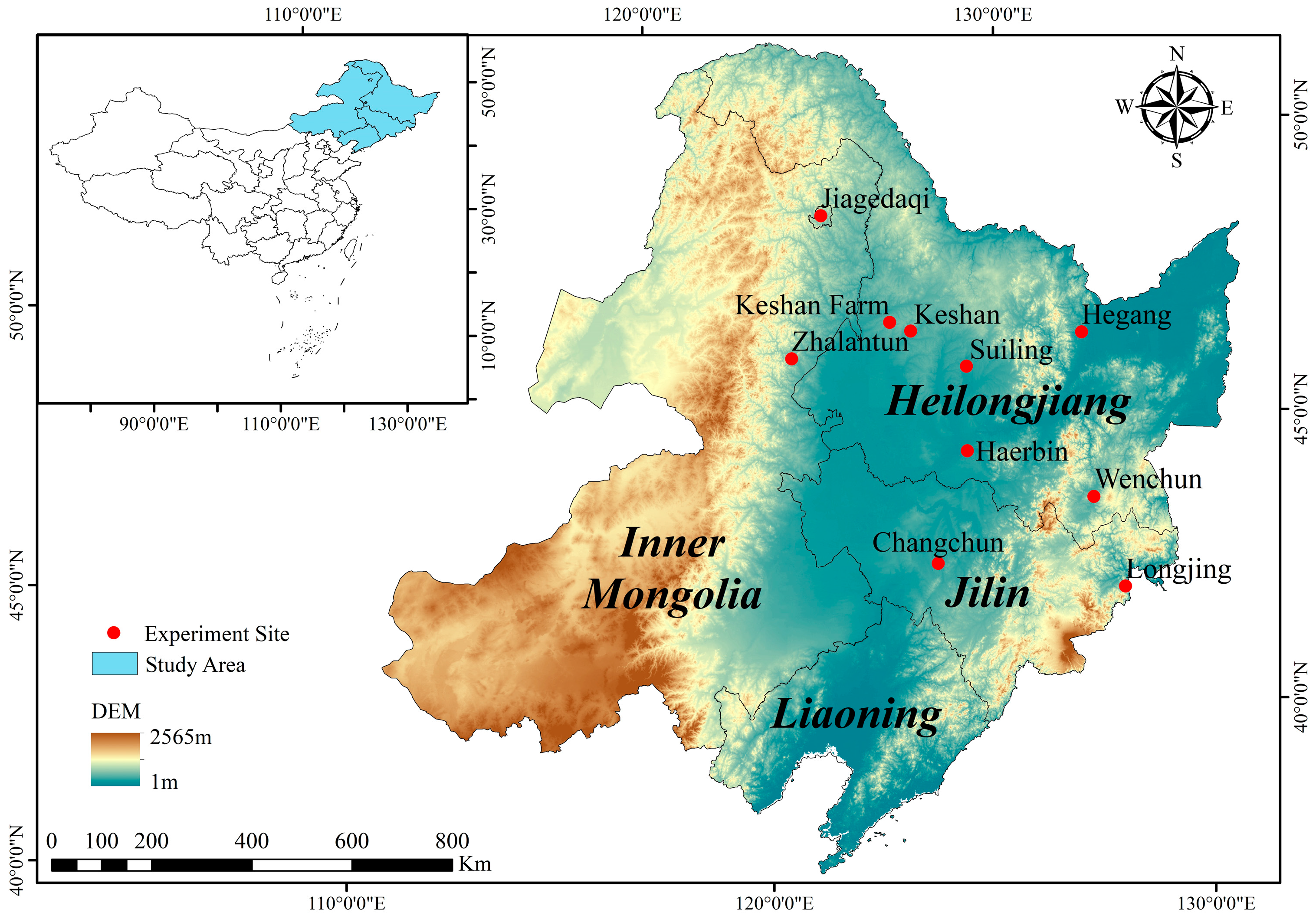
2.1. Field Experiments

The study area is located in the northeast subregion of the Northern Single-Cropping Zone (NSCZ) of potatoes in China (Figure 1), with a temperate continental monsoon climate and seasonal weather variations. This zone includes the Heilongjiang, Jilin, Eastern Inner Mongolia, and Liaoning Provinces. It is one of the main production areas for fresh vegetable varieties and one of the main potato starch processing areas [39].
Field experiments were conducted at the ten observation stations for the period of 2016–2020 (Table 1), which are part of the northeast group of the national potato variety regional trials [40], and the experimental area for each station was 700 m2. The potato variety in this study was Kexin #13 with medium-to-late maturation characteristics. Three replicates were conducted in each experimental field. The average yield was 35 tons per hectare, and the average growing period was 120 days within the same trial group, according to a unified experimental plan and technical operating procedures. The sowing depth was 22 cm with a plant distance of 30 cm, while the sowing density reached 60,000 plants/hm2. The sowing and harvest dates for each station were obtained in terms of actual records. Fertilization was performed in the initial stage of tuber formation with an amount equal to 130 kg/hm2. The observed data derived from the experiment were the average value of the three replicates.

2.2. DSSAT-SUBSTOR Model Inputs

In this study, the DSSAT-SUBSTOR model and potato genotypic parameters were selected. DSSAT-SUBSTOR is a process-based crop model that has been tested and applied in various potato-producing areas of China [41,42,43]. It can simulate potato phenology and yield based on potato genotypic parameters, weather, soil, and field management data.
The meteorological data inputs required by the DSSA-SUBSTOR model include the daily maximum temperature (°C), the daily minimum temperature (°C), daily radiation (MJ·m−2·d−1), and daily precipitation (mm), which were obtained from the China Meteorological Administration (http://www.cma.gov.cn/, accessed on 31 October 2023). Soil data derived from the China Soil Database (http://vdb3.soil.csdb.cn/, accessed on 31 October 2023) were pH, field capacity (g/cm3), saturated water content (g/cm3), bulk density in the different soil layers (g/cm3), organic matter content (g/cm3), and other basic parameters [44]. The management data for the model included the seeding method, planting density, sowing and harvesting dates, fertilization and irrigation amounts and dates, etc., which were generally derived from experimental records. In addition, genotypic parameters for potatoes are shown in Table 2 [45].

2.3. Sampling Methods and Sampling Design Framework

2.3.1. Introduction to Sampling Methods

The hold-out (HO), cross-validation (CA), and bootstrapping (BS) sampling methods were selected in this study to analyze the differences in the effectiveness of calibration results for SUBSTOR genotypic parameters. The sampling demonstration for the three methods is shown in Figure 2. HO is a method in which samples are directly taken from the sample pool, not returned, and divided into calibration and validation groups. The calibrated samples group is used to estimate genotypic parameters, while the validated samples group is used to test the assessment accuracy and precision [46]. CA is a method in which the sample pool is, through hierarchical sampling, divided into k subdatasets that have similar sizes and are mutually exclusive. One sample subdataset is the validation group, while the remaining k-1 sample subdatasets are calibration groups for each round of sampling. After calibration and validation over K iterations, the mean value is regarded as the final output. This technique is advantageous because it minimizes the variance linked to a single train/test split, thereby offering a more accurate assessment of the model’s performance [47]. BS is a method of sampling with replacement. There are a total of m samples in the initial pool, and n samples are randomly taken out and put back N times (n ≤ m). After N times, some original samples may be selected multiple times, while others might not be selected at all. The samples that are not selected can be used as a validation set for assessing the performance of the model, whereas the selected samples form the calibration set, used for training and tuning the model [48].

2.3.2. Sampling Design Framework

In terms of research requirements and because of differences in the quality of data used in field experiments, sample data from Harbin, Wenchun, Zhalantun, Keshan, Suiling, Hegang, Jiage, and Keshan Farm for 2016 to 2020 and from Changchun and Longjing for 2016, 2018, 2019, and 2020 were used. Thus, a total of 48 samples were applied in this study (Table 1). A comparison of the calibration results of the three sampling methods was conducted for each of the eight observation stations mentioned above, and the differences in results derived from the eight observation stations caused by using a single sampling method were analyzed. In addition, the differences in 48 samples were used to compare the calibration results of the genotypic parameters by using the three sampling methods.
To maintain the consistency of the sample data distribution before and after sampling and according to the sampling principle and the capacity of the original samples, the percentage of total samples for validation was uniformly 20–40% and for calibration was 60–80%. However, calibration and validation samples can be partitioned into groups in many ways. The estimation results obtained by using a single sampling method are often not stable and reliable. Thus, numerous random partitions were adopted, and at least five calibration sample groups for each sampling method were used in the GLUE module of the DSSA-SUBSTOR model for generic parameter estimation. After the genotypic parameters were determined for the five calibration sample groups, the results could be tested based on the validation sample group. Finally, the average values of the calibrated genotypic parameters were selected as the estimated values for the sampling method.
The specific sampling process is shown in Table 3 and Table 4. In single-station sampling (Table 3), the HO method randomly selects data from 3 years as the calibration set and from the remaining 2 years as the validation set. For the CA method, we set k = 5 to perform five-fold cross-validation. In this process, the five years are divided into five equal subsets with a 4:1 split. The crop model is calibrated based on four years and validated based on the remaining year. This procedure is repeated five times, with each subset used exactly once as the validation set. The BS sampling method with replacement obtains data proportions of 3:2 and 4:1 for the calibration and validation sets. Given the characteristics of sampling with replacement, some years will be repeatedly sampled, and the proportion of the dataset division will not be exactly the same each time.
In multi-station sampling (Table 4), we treat all trials across all sites and years as a single total sample set with a size of 48 and then apply each of the three sampling methods to this sample set. For the HO method, 5 samples were established without replacement from all 48 samples to obtain five different calibration and validation sets. The difference from single-station sampling lies in the range of division ratios. The random division is conducted with 60–80% of the samples forming the calibration set and 20–40% as the validation set. For the CA method, 48 samples were divided into 5 subsets by year, rotating 1 subset as the validation set and the others as the calibration sets. The specific process is the same as for a single station. For the BS method, 5 samples were conducted with replacement for all 48 samples to obtain 5 different calibration and validation sets. Given the differences in sampling methods, the proportions of calibration and validation samples were not completely consistent. However, the abovementioned 20–40% and 60–80% proportions were maintained for the validation set and the calibration set.

2.4. Genotypic Parameter Calibration and Validation

In this study, the generalized likelihood uncertainty estimation (GLUE) method embedded in DSSAT was used to estimate genotypic parameters [49]. The GLUE module runs over 6000 iterations to obtain a group of genotypic parameters. Based on calibrated generic parameters and the observation input data for validation, the DSSAT-SUBSTOR model can simulate yield values for validation. The root mean square error (RMSE) and the relative root mean square error (RRMSE) were used to analyze the error between the simulated and observed yields for each sampling result (Equations (1) and (2)). The average value of the errors for all the samplings was the final estimated error.
R M S E = i = 1 n S i R i 2 n
R R M S E = i = 1 n S i R i 2 n R ¯ × 100 %
Ri is the observation yield value; Si is the simulated yield value; n is the number of validation samples; and R ¯ is the average value of the observation yield. It is generally believed that the smaller the RMSE and RRMSE values are, the better the consistency between the simulated and the observation values. In this study, R language version 4.1.2, Origin 2023, and WPS version 11.1.0.14309 were used for data processing.

3. Results

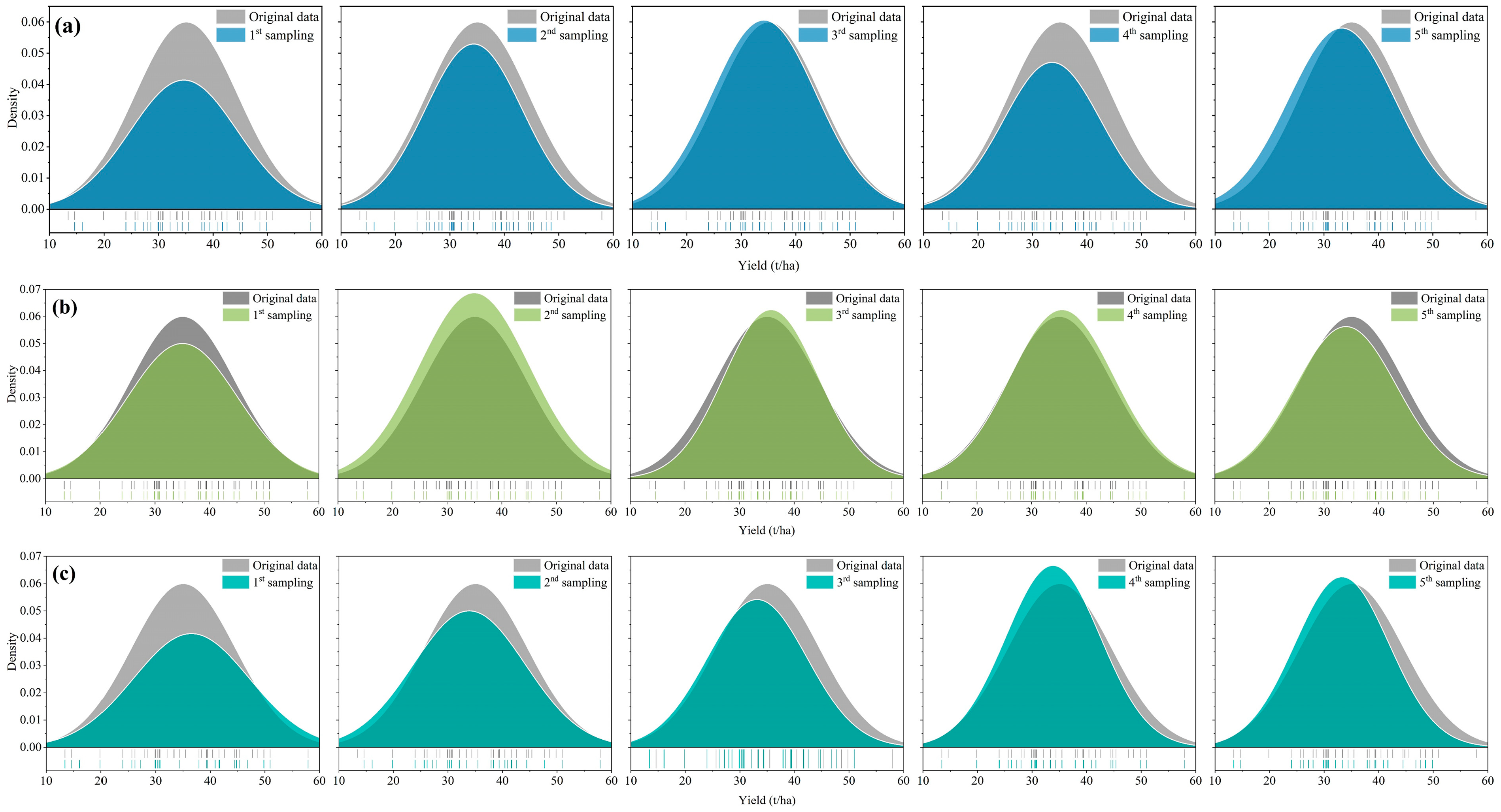
3.1. Statistical Distribution Consistency Analysis of Calibration Set and Original Sample Data

To avoid additional bias in calibration and validation sample data partitioning, the statistical distributions of all sample data before and after partitioning need to be as consistent as possible to ensure the generalizability of the DSSAT-SUBSTOR model for all sample data and to obtain better calibration results. Figure 3 shows the statistical distributions of all sample data before and after partitioning with the three sampling methods; these distributions were very consistent with each other and were suitable for subsequent genotypic parameter calibration. The overlap between the post-sampling fitting curve and the prior fitting curve exceeded 91% in all instances, which demonstrated that the calibration sample data were consistent with the original data and could be applied.

3.2. Validation of the Calibrated Yield Results Obtained with the Three Sampling Methods for Data from Each of the Observation Stations

The validation results for the RMSE and RRMSE of the yields and their coefficient of variation (CV) values are shown in Table 5, while the correlation analysis is depicted in Appendix A, Figure A1, Figure A2 and Figure A3. In terms of the RMSE and RRMSE from Table 5, the validation accuracies of the calibrated results obtained with the three sampling methods for a single observation station differed from each other. The performance of CA was best for the observation stations in Zhalantun, Hegang, Suiling, Keshan Farm, and Haerbin, and the accuracy of BS was highest for Chunshan and Keshan. HO was better than the other two methods for Jiagedaqi only. For Haerbin station, the CV values of RMSE and RRMSE were both approximately 10%, lower than those of the other stations except for Keshan, which indicated that the gap in the validation accuracy of the calibrated results obtained with the three methods was small. However, the RMSE and RRMSE for Haerbin were the highest among the eight stations, which suggested that the quality of the data obtained at Haerbin was not sufficient. Compared with Haerbin, the data quality for Hegang and Keshan was much better. The CV values of the RMSE and RRMSE showed that the differentiation of the validation accuracy of the calibrated results obtained with the three sampling methods at the eight stations varied. A value of 6.07% for Keshan Farm indicated that the effectiveness of the three sampling methods for calibrating genotypic parameters varied little, and the CV values of the RMSE and RRMSE were greater than 20% at Zhalantun, Wenchun, Hegang, and Keshan, which indicated that the prudent selection of the sampling method was necessary. According to relevant research on the performance evaluation of the DSSAT-SUBSTOR model, the average RMSE and RRMSE values of the tuber fresh weight of potatoes are 5.23 t/ha and 21%, respectively. The calibration results of this study are consistent with the accuracy of existing studies [50]. In addition, the CV values of the RMSE and RRMSE were quite different at various geospatial locations, which suggested that environmental variables impact the differentiation of the calibrated results obtained with the three methods.

3.3. CV Values of Calibrated Genotypic Parameters for the Three Sampling Methods

As shown in Table 6 and Table 7, the CV values for the five genotypic parameters differentiated from each other for each of the eight observation stations, and the CV values of the calibrated single genotypic parameters at all eight observation stations derived from the three sampling methods were similar; however, these values varied greatly between the genotypic parameters. Compared with the other four parameters, the CV values of the calibrated results obtained with the three sampling methods for all eight observation stations were the lowest, which verified that the G3 value had little effect on the geographic and environmental variables. The CV value of P2 was the highest among the five genotypic parameters, suggesting that P2, which influences the phenology of potato growth, is affected most by natural and ecological elements. In terms of Table 6, there was no obvious regularity in the sequence of the CV values of the five genotypic parameters for each station. In Table 7, compared with those of parameters G3, PD, and TC, the CVs of P2 and G2 for the three methods were the lowest, which showed that the calibrated results for each of the two parameters obtained with the three sampling methods were similar. Moreover, the calibrated result for TC was the opposite, with a maximum value of 21.04%. Overall, HO, CA, and BS displayed different calibration effectiveness values for the five genotypic parameters.

3.4. Comparison of Validation Results for Calibrated Genotypic Parameters Obtained with the Three Sampling Methods Using All 48 Samples

In terms of the averaged RMSE and RRMSE values in Table 8, the validation accuracy of the calibrated genotypic parameters obtained using all 48 samples was not better than that obtained with the samples from a single observation station, which may have been caused by the difference in data quality between the different stations. The CVs of the RMSE and RRMSE values derived from 15 sets of data (Table 8) obtained with the three sampling methods were 26.80% and 26.89%, much higher than 16.64% and 20.07, respectively, which were the average values of the corresponding CVs obtained with data from a single observation station (except for Keshan station). The results showed that, as the number of samples increased, the difference in validation accuracy for calibrating genotypic parameters with the three methods increased. For genotypic parameter calibration, CV values for multi-station data obtained with the three methods were quite different from those for single-station data (Table 8); this verified that calibration results derived from data from a single station are inferior to those obtained using all 48 samples, and the genotypic parameter calibration results varied greatly because of different manipulation pathways and sample use strategies.

4. Discussion

Sample size and sampling methods are seldom discussed when the genotypic parameters of crop growth models are calibrated. The default method for dividing samples for calibration and validation is the HO method. However, our findings suggest that different sample sizes and sampling methods are superior in certain cases, thus influencing the calibration and validation results for genotypic parameters. For small sample sizes, the calibration and validation results derived from the HO, CA, and BS methods varied greatly. With an increasing sample size, the gap between the calibration and validation results among the three methods did not narrow. In addition, for the different geographic locations, the calibration and validation results obtained with the three methods were different, and the HO method was not the best after the test. Notably, the mechanism of the three methods of sampling differed, and the information exploration and sample use strategies highly varied, especially for small sample sizes. Compared with the HO method, CA and BS are more suitable for cases with small sample sizes. The abovementioned results verified that, in the calibration and validation of genotypic parameters, sample methods and sample sizes should be considered.
In this study, RMSE, RRMSE, and the CVs of RMSE and RRMSE for the eight observation stations did not show any obvious geographic regularity with ascending latitude and elevation. However, because of differences in data quality, the RMSE and RRMSE for each of the stations differed greatly. Except for those of Haerbin station, the RMSE and RRMSE values of each single observation station were lower than the average RMSE and RRMSE values derived from the 48 samples. Thus, genotypic parameter calibration should be performed with data from a single observation station only if the corresponding RMSE and RRMSE values are small.
The calibration results of the five genotypic parameters obtained with the three sampling methods and using different sample sizes were quite different. For G3, the CVs of the calibrated results obtained with the three sampling methods for the eight observation stations were lower than 4%, as shown in Table 5, and the CVs of P2 were all greater than 30%. The fluctuation in CVs among the eight stations was affected not only by input data quality but also by the value range of each genotypic parameter. The value range of G3 should be much narrower than that of the other four genotypic parameters, and the calibration results for G3 were not affected by geographic or environmental elements; in contrast, P2 was considerably influenced by natural ecological indicators. Although the CV of the calibration results for P2 at the eight stations was the largest, the values obtained with different methods varied little. Compared with P2, the variations in G2 among the three methods were obvious.
Given the differences in quality from the different stations, we could not conclude that the more samples there were, the better the calibration result would be. In cases based on the genotypic parameter calibration results from a single observation station or a small sample size, not only the RMSE and RRMSE values but also the CV of the validation accuracy of the calibration results obtained with the three methods should be considered. If the RMSE and RRMSE meet the relevant accuracy requirements, and the CV of the calibration results is small, the calibrated genotypic parameters are likely suitable. In this study, the genotypic parameters calibrated for Keshan seemed optimal for use. For genotypic parameter calibration results from a large sample pool, since there was abundant sample information, the effectiveness of the three sample methods varied. The RMSE and RRMSE values were considered the main indicators of final genotypic parameter calibration in such cases. Although the calibration results from a single observation station seemed acceptable, overfitting may have occurred [51]. Thus, if possible, large samples with high-quality data are still needed.
One limitation of this study was a lack of observed phenological data. Since phenological data were not available, we used yield, a single indicator, to perform calibration. In addition, uncertainty existed in the process of sampling; for instance, the percentage of partitioned samples can be manipulated by users. To control variables and reduce the unreasonableness of sample partitioning, a fixed percentage was adopted in the sampling procedure in this study; therefore, the influence of the sample-partitioning percentage on sampling was ignored. In future studies, the sampling percentage should be fully considered.

5. Conclusions

Generic parameter calibration for crop growth models is a very important step in model use. Scientists generally apply the HO method, by default, to obtain samples for calibration and validation in practical model use. Our results indicate that the size of the sample sets used for calibration and validation and the sampling method have very important effects on the final calibration results for genotypic parameters. First, at the different observation stations, it was difficult to conclude which of the HO, CA, and BS methods performed best. Moreover, CA and BS outperformed the HO method at most observation stations, suggesting that the sampling method should be appropriately selected before calibrating genotypic parameters. In addition, as the sampling size increased, the effectiveness of calibration with the three methods showed increased differentiation. Given data quality differences, we could not conclude that the greater the number of samples there were, the greater the validation accuracy of the three methods. The CVs of the genotypic parameter values derived from the three methods and sample sizes varied greatly, and this variation was also affected by the value ranges selected and the natural environmental conditions. Thus, when genotypic parameter calibration is performed, both the sampling methods and sample size should be seriously considered.

Author Contributions

Conceptualization, Y.H.; data curation, X.W. and H.C.; funding acquisition, Y.H.; methodology, Y.Z.; project administration, Y.H.; resources, H.C. and S.H.; software, X.M.; supervision, X.M.; visualization, S.H.; writing—original draft, X.M. and X.W.; writing—review and editing, Y.Z. All authors have read and agreed to the published version of the manuscript.

Funding

This research was funded by the National Natural Science Foundation of China “Study on temporally and spatially precise assessment on potato cultivation suitability based on dynamic process-oriented mode” (41771562); the Agricultural Science and Technology Innovation Program (G2023-18-2); and the Fundamental Research Funds for Central Non-profit Scientific Institution (G2023-01-27).

Institutional Review Board Statement

Not applicable.

Data Availability Statement

Data are contained within the article.

Conflicts of Interest

The authors declare no conflict of interest.

Appendix A

Validation results of the three sampling methods for single- and multi-station data.
Figure A1. Validation results of the HO sampling methods for single- and multi-station data: (a) represents single-station data, and (b) represents multi-station data.
Agriculture 13 02207 g0a1
Figure A2. Validation results of the CA sampling methods for single- and multi-station data: (a) represents single-station data, and (b) represents multi-station data.
Agriculture 13 02207 g0a2
Figure A3. Validation results of the BS sampling methods for single- and multi-station data: (a) represents single-station data, and (b) represents multi-station data.
Agriculture 13 02207 g0a3

References

  1. Farina, R.; Sándor, R.; Abdalla, M.; Álvaro-Fuentes, J.; Bechini, L.; Bolinder, M.A.; Brilli, L.; Chenu, C.; Clivot, H.; De Antoni Migliorati, M.; et al. Ensemble Modelling, Uncertainty and Robust Predictions of Organic Carbon in Long-term Bare-fallow Soils. Glob. Chang. Biol. 2021, 27, 904–928. [Google Scholar] [CrossRef] [PubMed]
  2. Sándor, R.; Ehrhardt, F.; Grace, P.; Recous, S.; Smith, P.; Snow, V.; Soussana, J.-F.; Basso, B.; Bhatia, A.; Brilli, L.; et al. Ensemble Modelling of Carbon Fluxes in Grasslands and Croplands. Field Crops Res. 2020, 252, 107791. [Google Scholar] [CrossRef]
  3. Seidel, S.J.; Palosuo, T.; Thorburn, P.; Wallach, D. Towards Improved Calibration of Crop Models—Where Are We Now and Where Should We Go? Eur. J. Agron. 2018, 94, 25–35. [Google Scholar] [CrossRef]
  4. Porwollik, V.; Müller, C.; Elliott, J.; Chryssanthacopoulos, J.; Iizumi, T.; Ray, D.K.; Ruane, A.C.; Arneth, A.; Balkovič, J.; Ciais, P.; et al. Spatial and Temporal Uncertainty of Crop Yield Aggregations. Eur. J. Agron. 2017, 88, 10–21. [Google Scholar] [CrossRef]
  5. Huang, J.; Gómez-Dans, J.L.; Huang, H.; Ma, H.; Wu, Q.; Lewis, P.E.; Liang, S.; Chen, Z.; Xue, J.-H.; Wu, Y.; et al. Assimilation of Remote Sensing into Crop Growth Models: Current Status and Perspectives. Agric. For. Meteorol. 2019, 276–277, 107609. [Google Scholar] [CrossRef]
  6. Walker, W.E.; Harremoës, P.; Rotmans, J.; Sluijs, J.P.; van der Asselt, M.B.A.; van Janssen, P.; von Krauss, M.P.K. Defining Uncertainty: A Conceptual Basis for Uncertainty Management in Model-Based Decision Support. Integr. Assess. 2003, 4, 5–17. [Google Scholar] [CrossRef]
  7. Wallach, D.; Thorburn, P.; Asseng, S.; Challinor, A.J.; Ewert, F.; Jones, J.W.; Rotter, R.; Ruane, A. Estimating Model Prediction Error: Should You Treat Predictions as Fixed or Random? Environ. Model. Softw. 2016, 84, 529–539. [Google Scholar] [CrossRef]
  8. Tao, F.; Rötter, R.P.; Palosuo, T.; Gregorio Hernández Díaz-Ambrona, C.; Mínguez, M.I.; Semenov, M.A.; Kersebaum, K.C.; Nendel, C.; Specka, X.; Hoffmann, H.; et al. Contribution of Crop Model Structure, Parameters and Climate Projections to Uncertainty in Climate Change Impact Assessments. Glob. Chang. Biol. 2018, 24, 1291–1307. [Google Scholar] [CrossRef]
  9. Wallach, D.; Thorburn, P.J. Estimating Uncertainty in Crop Model Predictions: Current Situation and Future Prospects. Eur. J. Agron. 2017, 88, A1–A7. [Google Scholar] [CrossRef]
  10. Ramirez-Villegas, J.; Koehler, A.-K.; Challinor, A.J. Assessing Uncertainty and Complexity in Regional-Scale Crop Model Simulations. Eur. J. Agron. 2017, 88, 84–95. [Google Scholar] [CrossRef]
  11. Chapagain, R.; Remenyi, T.A.; Harris, R.M.B.; Mohammed, C.L.; Huth, N.; Wallach, D.; Rezaei, E.E.; Ojeda, J.J. Decomposing Crop Model Uncertainty: A Systematic Review. Field Crops Res. 2022, 279, 108448. [Google Scholar] [CrossRef]
  12. Ma, L.; Malone, R.W.; Heilman, P.; Ahuja, L.R.; Meade, T.; Saseendran, S.A.; Ascough, J.C.; Kanwar, R.S. Sensitivity of Tile Drainage Flow and Crop Yield on Measured and Calibrated Soil Hydraulic Properties. Geoderma 2007, 140, 284–296. [Google Scholar] [CrossRef]
  13. Varella, H.; Buis, S.; Launay, M.; Guérif, M. Global Sensitivity Analysis for Choosing the Main Soil Parameters of a Crop Model to Be Determined. Agric. Sci. 2012, 3, 24661. [Google Scholar] [CrossRef]
  14. Rosenzweig, C.; Elliott, J.; Deryng, D.; Ruane, A.C.; Müller, C.; Arneth, A.; Boote, K.J.; Folberth, C.; Glotter, M.; Khabarov, N.; et al. Assessing Agricultural Risks of Climate Change in the 21st Century in a Global Gridded Crop Model Intercomparison. Proc. Natl. Acad. Sci. USA 2014, 111, 3268–3273. [Google Scholar] [CrossRef] [PubMed]
  15. Wang, X.X.; He, J.R.; Williams, R.C.; Izaurralde, J.D. Atwood sensitivity and uncertainty analyses of crop yields and soil organic carbon simulated with epic. Trans. ASAE 2005, 48, 1041–1054. [Google Scholar] [CrossRef]
  16. Araya, A.; Hoogenboom, G.; Luedeling, E.; Hadgu, K.M.; Kisekka, I.; Martorano, L.G. Assessment of Maize Growth and Yield Using Crop Models under Present and Future Climate in Southwestern Ethiopia. Agric. For. Meteorol. 2015, 214–215, 252–265. [Google Scholar] [CrossRef]
  17. Deb, P.; Kiem, A.S.; Babel, M.S.; Chu, S.T.; Chakma, B. Evaluation of Climate Change Impacts and Adaptation Strategies for Maize Cultivation in the Himalayan Foothills of India. J. Water Clim. Chang. 2015, 6, 596–614. [Google Scholar] [CrossRef]
  18. Li, Z.; He, J.; Xu, X.; Jin, X.; Huang, W.; Clark, B.; Yang, G.; Li, Z. Estimating Genetic Parameters of DSSAT-CERES Model with the GLUE Method for Winter Wheat (Triticum aestivum L.) Production. Comput. Electron. Agric. 2018, 154, 213–221. [Google Scholar] [CrossRef]
  19. Pathak, T.B.; Jones, J.W.; Fraisse, C.W.; Wright, D.; Hoogenboom, G. Uncertainty Analysis and Parameter Estimation for the CSM-CROPGRO-Cotton Model. Agron. J. 2012, 104, 1363–1373. [Google Scholar] [CrossRef]
  20. Sun, M.; Zhang, X.; Huo, Z.; Feng, S.; Huang, G.; Mao, X. Uncertainty and Sensitivity Assessments of an Agricultural–Hydrological Model (RZWQM2) Using the GLUE Method. J. Hydrol. 2016, 534, 19–30. [Google Scholar] [CrossRef]
  21. Jin, X.; Li, Z.; Nie, C.; Xu, X.; Feng, H.; Guo, W.; Wang, J. Parameter Sensitivity Analysis of the AquaCrop Model Based on Extended Fourier Amplitude Sensitivity under Different Agro-Meteorological Conditions and Application. Field Crops Res. 2018, 226, 1–15. [Google Scholar] [CrossRef]
  22. Tan, J.; Cao, J.; Cui, Y.; Duan, Q.; Gong, W. Comparison of the Generalized Likelihood Uncertainty Estimation and Markov Chain Monte Carlo Methods for Uncertainty Analysis of the ORYZA_V3 Model. Agron. J. 2019, 111, 555–564. [Google Scholar] [CrossRef]
  23. Cooman, A.; Schrevens, E. A Monte Carlo Approach for Estimating the Uncertainty of Predictions with the Tomato Plant Growth Model, Tomgro. Biosyst. Eng. 2006, 94, 517–524. [Google Scholar] [CrossRef]
  24. Dzotsi, K.A.; Basso, B.; Jones, J.W. Parameter and Uncertainty Estimation for Maize, Peanut and Cotton Using the SALUS Crop Model. Agric. Syst. 2015, 135, 31–47. [Google Scholar] [CrossRef]
  25. Wallach, D.; Thorburn, P.J. The Error in Agricultural Systems Model Prediction Depends on the Variable Being Predicted. Environ. Model. Softw. 2014, 62, 487–494. [Google Scholar] [CrossRef]
  26. Ines, A.V.M.; Honda, K.; Das Gupta, A.; Droogers, P.; Clemente, R.S. Combining Remote Sensing-Simulation Modeling and Genetic Algorithm Optimization to Explore Water Management Options in Irrigated Agriculture. Agric. Water Manag. 2006, 83, 221–232. [Google Scholar] [CrossRef]
  27. Dong, T.; Liu, J.; Qian, B.; Zhao, T.; Jing, Q.; Geng, X.; Wang, J.; Huffman, T.; Shang, J. Estimating Winter Wheat Biomass by Assimilating Leaf Area Index Derived from Fusion of Landsat-8 and MODIS Data. Int. J. Appl. Earth Obs. Geoinf. 2016, 49, 63–74. [Google Scholar] [CrossRef]
  28. Jin, X.; Li, Z.; Yang, G.; Yang, H.; Feng, H.; Xu, X.; Wang, J.; Li, X.; Luo, J. Winter Wheat Yield Estimation Based on Multi-Source Medium Resolution Optical and Radar Imaging Data and the AquaCrop Model Using the Particle Swarm Optimization Algorithm. ISPRS J. Photogramm. Remote Sens. 2017, 126, 24–37. [Google Scholar] [CrossRef]
  29. Silvestro, P.C.; Pignatti, S.; Pascucci, S.; Yang, H.; Li, Z.; Yang, G.; Huang, W.; Casa, R. Estimating Wheat Yield in China at the Field and District Scale from the Assimilation of Satellite Data into the Aquacrop and Simple Algorithm for Yield (SAFY) Models. Remote Sens. 2017, 9, 509. [Google Scholar] [CrossRef]
  30. Jégo, G.; Pattey, E.; Liu, J. Using Leaf Area Index, Retrieved from Optical Imagery, in the STICS Crop Model for Predicting Yield and Biomass of Field Crops. Field Crops Res. 2012, 131, 63–74. [Google Scholar] [CrossRef]
  31. Dente, L.; Satalino, G.; Mattia, F.; Rinaldi, M. Assimilation of Leaf Area Index Derived from ASAR and MERIS Data into CERES-Wheat Model to Map Wheat Yield. Remote Sens. Environ. 2008, 112, 1395–1407. [Google Scholar] [CrossRef]
  32. He, B.; Li, X.; Quan, X.; Qiu, S. Estimating the Aboveground Dry Biomass of Grass by Assimilation of Retrieved LAI Into a Crop Growth Model. IEEE J. Sel. Top. Appl. Earth Obs. Remote Sens. 2015, 8, 550–561. [Google Scholar] [CrossRef]
  33. Jin, H.; Li, A.; Wang, J.; Bo, Y. Improvement of Spatially and Temporally Continuous Crop Leaf Area Index by Integration of CERES-Maize Model and MODIS Data. Eur. J. Agron. 2016, 78, 1–12. [Google Scholar] [CrossRef]
  34. Curnel, Y.; de Wit, A.J.W.; Duveiller, G.; Defourny, P. Potential Performances of Remotely Sensed LAI Assimilation in WOFOST Model Based on an OSS Experiment. Agric. For. Meteorol. 2011, 151, 1843–1855. [Google Scholar] [CrossRef]
  35. Roux, S.; Brun, F.; Wallach, D. Combining Input Uncertainty and Residual Error in Crop Model Predictions: A Case Study on Vineyards. Eur. J. Agron. 2014, 52, 191–197. [Google Scholar] [CrossRef]
  36. Ibrahim, O.M.; Gaafar, A.A.; Wali, A.M.; Tawfik, M.M.; El-Nahas, M.M. Estimating Cultivar Coefficients of a Spring Wheat Using GenCalc and GLUE in DSSAT. J. Agron. 2016, 15, 130–135. [Google Scholar] [CrossRef]
  37. Tao, F.; Zhang, Z.; Liu, J.; Yokozawa, M. Modelling the Impacts of Weather and Climate Variability on Crop Productivity over a Large Area: A New Super-Ensemble-Based Probabilistic Projection. Agric. For. Meteorol. 2009, 149, 1266–1278. [Google Scholar] [CrossRef]
  38. Trnka, M.; Dubrovský, M.; Semerádová, D.; Žalud, Z. Projections of Uncertainties in Climate Change Scenarios into Expected Winter Wheat Yields. Theor Appl Clim. 2004, 77, 229–249. [Google Scholar] [CrossRef]
  39. Wang, Z. Potato Processing Industry in China: Current Scenario, Future Trends and Global Impact. Potato Res. 2023, 66, 543–562. [Google Scholar] [CrossRef]
  40. Na, T. Analysis of Accuracy and Stability in Regional Trial of Potato Varieties. Chin. Acad. Agric. Sci. 2011. Available online: https://www.cnki.net/KCMS/detail/detail.aspx?dbcode=CMFD&dbname=CMFD2012&filename=1012318224.nh&uniplatform=OVERSEA&v=3HNO6lOT58LlKVk4qABr8jWx3PCs11KNuQbKz2gjn0g-iepASYD5CjSi8R6hXY7p (accessed on 31 October 2023).
  41. Duan, D.; YingBin, H.; JinKuan, Y.; Li, L.; RuiYang, X.; WenJuan, L. Parameter Sensitivity Analysis and Suitability Evaluation of DSSAT-SUBSTOR Potato Model. J. Anhui Agric. Univ. 2019, 46, 521–527. [Google Scholar]
  42. Gao, F.; Luan, X.; Yin, Y.; Sun, S.; Li, Y.; Mo, F.; Wang, J. Exploring Long-Term Impacts of Different Crop Rotation Systems on Sustainable Use of Groundwater Resources Using DSSAT Model. J. Clean. Prod. 2022, 336, 130377. [Google Scholar] [CrossRef]
  43. Wang, H.; Cheng, M.; Liao, Z.; Guo, J.; Zhang, F.; Fan, J.; Feng, H.; Yang, Q.; Wu, L.; Wang, X. Performance Evaluation of AquaCrop and DSSAT-SUBSTOR-Potato Models in Simulating Potato Growth, Yield and Water Productivity under Various Drip Fertigation Regimes. Agric. Water Manag. 2023, 276, 108076. [Google Scholar] [CrossRef]
  44. Fleisher, D.H.; Cavazzoni, J.; Giacomelli, G.A.; Ting, K.C. Adaptation of SUBSTOR for Controlled-Environment Potato Production with Elevated Carbon Dioxide. Trans. ASAE 2003, 46, 531–538. [Google Scholar] [CrossRef] [PubMed]
  45. Griffin, T.S.; Johnson, B.S.; Ritchie, J.T.; IBSNAT Project; University of Hawaii (Honolulu); Department of Agronomy and Soil Science; Michigan State University, Department of Crop and Soil Science. A Simulation Model for Potato Growth and Development: SUBSTOR-Potato Version 2.0; IBSNAT Research Report Series; Michigan State University, Department of Crop and Soil Sciences: East Lansing, MI, USA, 1993. [Google Scholar]
  46. Zhou, Z. Machine Learning; Tsinghua University Press: Beijing, China, 2016. [Google Scholar]
  47. Dietterich, T.G. Approximate Statistical Tests for Comparing Supervised Classification Learning Algorithms. Neural Comput 1998, 10, 1895–1923. [Google Scholar] [CrossRef] [PubMed]
  48. Efron, B.; Tibshirani, R.J. An Introduction to the Bootstrap; Chapman and Hall/CRC: Broken Sound Parkway, NW, USA, 1994; ISBN 978-0-429-24659-3. [Google Scholar]
  49. Jones, J.W.; He, J.; Boote, K.J.; Wilkens, P.; Porter, C.H.; Hu, Z. Estimating DSSAT Cropping System Cultivar-Specific Parameters Using Bayesian Techniques. In Advances in Agricultural Systems Modeling; Ahuja, L.R., Ma, L., Eds.; American Society of Agronomy and Soil Science Society of America: Madison, WI, USA, 2015; pp. 365–393. ISBN 978-0-89118-196-5. [Google Scholar]
  50. Raymundo, R. Performance of the SUBSTOR-Potato Model across Contrasting Growing Conditions. Field Crops Res. 2017, 202, 57–76. [Google Scholar] [CrossRef]
  51. Yang, Y.; Wilson, L.T.; Li, T.; Paleari, L.; Confalonieri, R.; Zhu, Y.; Tang, L.; Qiu, X.; Tao, F.; Chen, Y.; et al. Integration of Genomics with Crop Modeling for Predicting Rice Days to Flowering: A Multi-Model Analysis. Field Crops Res. 2022, 276, 108394. [Google Scholar] [CrossRef]
Figure 1. Locations of observation stations in the study area.
Agriculture 13 02207 g001
Figure 2. Sampling demonstration for the three methods. Note: The variable “D” in black represents the calibration set, the red “D” represents the validation set, and “D1” is the first sampling; “m” represents the total number of samples in the original dataset. In the BS method, “D′” represents the samples that were never selected for the validation dataset, and “D-D′” represents the selected samples for the calibration dataset.
Agriculture 13 02207 g002
Figure 3. The statistical distribution of sample data before and after sampling with the three methods: (a) represents the HO method, (b) represents the CA method, and (c) represents the BS method.
Agriculture 13 02207 g003
Table 1. Meteorological and experimental sites in this study.
Experimental SiteYearLongitude (°)Latitude (°)Altitude (m)Observed Yield (t/ha)GSL * (d)≥10 °C GDD *Soil Type
Haerbin2016–2020126.6345.7515532.8 ± 13.2 *114 ± 72243 ± 186SiLo *
Wenchun2016–2020129.5044.4225144.2 ± 3.9124 ± 42259 ± 85SiLo
Zhalantun2016–2020122.7448.0330737.4 ± 5.4131 ± 112240 ± 142ClLo *
Keshan2016–2020125.8748.0723627.6 ± 2.7113 ± 42252 ± 86SiClLo *
Keshan Farm2016–2020125.3748.3031547.1 ± 8121 ± 102251 ± 182SiClLo
Suiling2016–2020127.1047.2321235.9 ± 4.4107 ± 92254 ± 214SiClLo
Hegang2016–2020130.2747.3322831.1 ± 1.8123 ± 112258 ± 169SiLo
Jiagedaqi2016–2020124.1250.4037228.7 ± 6117 ± 72237 ± 105Lo *
Changchun2016, 2018–2020125.3243.8323734.7 ± 13.5124 ± 62266 ± 106SiLo
Longjing2016, 2018–2020129.7042.7024233.5 ± 9.2122 ± 52263 ± 77Lo
Note *: ≥10 °C GDD represents the accumulated growing degree days (GDD) above 10 °C. The number 32.8 ± 13.2 indicates the mean value (32.8) with a standard deviation of 13.2; GSL represents Growing Season Length (days); Lo: Loam; SiLo: Silty Loam; ClLo: Clay Loam; SiClLo: Silty Clay Loam.
Table 2. Genotypic parameters for potatoes in DSSAT.
Genotypic ParametersDefinitionType
G2 (cm2·m−2·d−1)Leaf expansion rateFor yield
G3 (g·m−2·d−1)Tuber growth rateFor yield
PDDeterminacyFor yield
P2Sensitivity of tuber initiation to photoperiodFor phenology
TC (°C)Coefficient for critical temperatureFor phenology
Table 3. Summary of sampling methods and selected years in single-station sampling.
Sampling Sequence NumberSampling MethodCalibration YearValidation Year
1HO2017, 2018, 20192016, 2020
22016, 2018, 20192017, 2020
32016, 2017, 20192018, 2020
42016, 2017, 20182019, 2020
52017, 2018, 20202016, 2019
6CA2017, 2018, 2019, 20202016
72016, 2018, 2019, 20202017
82016, 2017, 2019, 20202018
92016, 2017, 2018, 20202019
102016, 2017, 2018, 20192020
11BS2017, 2018, 2020, 2018, 20202016, 2019
122017, 2019, 2020, 2019, 20202016, 2018
132017, 2018, 2019, 2020, 20202016
142016, 2018, 2019, 2016, 20182017, 2020
152016, 2018, 2019, 2020, 20182017
Table 4. Summary of sampling methods and sample division in multi-station sampling.
Sampling Sequence NumberSampling MethodsCalibration SetValidation Set
1HO29 *19 **
234 *14 **
333 *15 **
434 *14 **
531 *17 **
6CA2017, 2018, 2019, 2020 ***2016 ****
72016, 2018, 2019, 2020 ***2017 ****
82016, 2017, 2019, 2020 ***2018 ****
92016, 2017, 2018, 2020 ***2019 ****
102016, 2017, 2018, 2019 ***2020 ****
11BS30 *18 **
1231 *17 **
1334 *14 **
1431 *17 **
1530 *18 **
Note: * indicates the number of calibration samples randomly selected from the 48 total samples; ** refers to the number of validation samples, which are the remaining samples after * selections. *** represents the years selected for calibrating genotypic parameters, and **** designates the years selected for validation.
Table 5. Accuracy comparison of calibration results obtained with the three sampling methods for each of the eight observation stations.
Observation StationSampling MethodsMean of RMSECV of RMSEMean of RRMSECV of RRMSE
ZhalantunHO8.7020.86%23.09%21.84%
CA5.7415.34%
BS8.1223.11%
WenchunHO6.3520.04%14.93%22.99%
CA4.5810.35%
BS4.5410.12%
HegangHO3.0126.63%9.45%25.04%
CA1.845.93%
BS2.096.73%
SuilingHO10.0615.17%31.87%18.32%
CA7.7324.40%
BS7.9022.83%
KeshanHO3.8237.45%13.55%37.41%
CA2.8910.48%
BS1.726.08%
Keshan FarmHO6.406.07%12.87%7.85%
CA5.9612.67%
BS6.7314.58%
JiagedaqiHO7.6016.94%25.22%18.35%
CA10.2535.70%
BS7.8927.96%
HaerbinHO14.5211.22%38.59%8.79%
CA11.6935.64%
BS13.9842.46%
Table 6. Calibrated genotypic parameters obtained with the three sampling methods and the corresponding CV for each observation station.
Observation StationSampling MethodG2G3PDP2TC
ZhalantunHO1772.5424.460.780.4816.98
CA1683.8023.620.680.5016.48
BS1779.3622.380.760.4216.44
CV3.05%4.46%7.15%8.92%1.81%
WenchunHO1384.0623.740.760.4017.50
CA1585.5623.521.000.4018.30
BS1329.6423.961.000.4017.70
CV9.41%0.93%15.06%0.00%2.33%
HegangHO1548.4823.280.840.6415.96
CA1266.1023.600.840.8017.56
BS1476.3223.020.960.8018.44
CV10.26%1.25%7.87%12.37%7.26%
SuilingHO1262.1822.940.600.8018.58
CA1576.1821.700.760.7419.44
BS1544.8422.960.680.8219.34
CV11.84%3.20%11.76%5.29%2.46%
KeshanHO1683.1423.720.880.8619.78
CA1835.7223.380.880.8419.10
BS1619.5823.001.000.9020.58
CV6.49%1.54%7.53%3.53%3.74%
Keshan FarmHO1597.3423.180.780.3418.86
CA1729.3023.800.600.3416.58
BS1810.8423.880.660.3616.88
CV6.29%1.62%13.48%3.33%7.10%
JiagedaqiHO1756.3821.980.920.7218.92
CA1460.3023.220.820.7218.80
BS1559.7022.640.780.7220.24
CV9.46%2.74%8.58%0.00%4.14%
HaerbinHO1633.2823.200.780.7216.84
CA1348.5823.300.920.5415.82
BS1764.5023.280.820.5615.18
CV13.44%0.23%8.58%16.26%5.25%
Table 7. CV of the five genotypic parameters for each of the three sampling methods for all eight observation stations.
Sampling MethodG2G3PDP2TC
HO11.28%3.08%12.14%30.89%7.26%
CA12.39%2.84%15.95%31.10%7.62%
BS10.40%2.39%16.59%34.37%10.51%
CV of CV8.82%12.75%16.17%6.06%21.04%
Table 8. RSME, RRMSE, and CVs for yield and genotypic parameters obtained with the three sampling methods using 48 samples.
Sampling Sequence NumberSampling MethodG2G3PDP2TCRMSERRMSE
1HO2044.4023.100.900.7018.208.8525.57%
2HO1230.4022.700.900.7018.3011.4533.32%
3HO1962.3025.000.800.7018.408.5425.00%
4HO2091.2025.801.000.7019.6010.8232.21%
5HO1729.4023.300.700.8020.109.5828.82%
Average1811.5423.980.860.7218.929.8528.98%
6CA1960.0024.000.600.7019.7011.1631.85%
7CA992.0021.900.900.7021.109.1926.28%
8CA1813.2023.401.000.5016.4012.8235.83%
9CA1902.1024.301.000.6017.708.2923.30%
10CA1790.0022.700.800.7017.2017.0450.11%
Average1691.4623.260.860.6418.4211.7033.48%
11BS990.7024.001.000.6018.307.0019.61%
12BS2193.3024.900.800.7018.307.9121.76%
13BS1702.0022.400.800.7016.9016.7545.88%
14BS1750.3021.800.600.8021.509.6026.95%
15BS1104.2025.500.800.8021.3010.7128.86%
Average1548.1023.720.800.7219.2610.3928.61%
CV23.22%5.17%15.55%11.13%8.25%26.80%26.89%
Disclaimer/Publisher’s Note: The statements, opinions and data contained in all publications are solely those of the individual author(s) and contributor(s) and not of MDPI and/or the editor(s). MDPI and/or the editor(s) disclaim responsibility for any injury to people or property resulting from any ideas, methods, instructions or products referred to in the content.

