
Simulating Soil–Disc Plough Interaction Using Discrete Element Method–Multi-Body Dynamic Coupling

Abstract
:1. Introduction
2. Materials and Methods
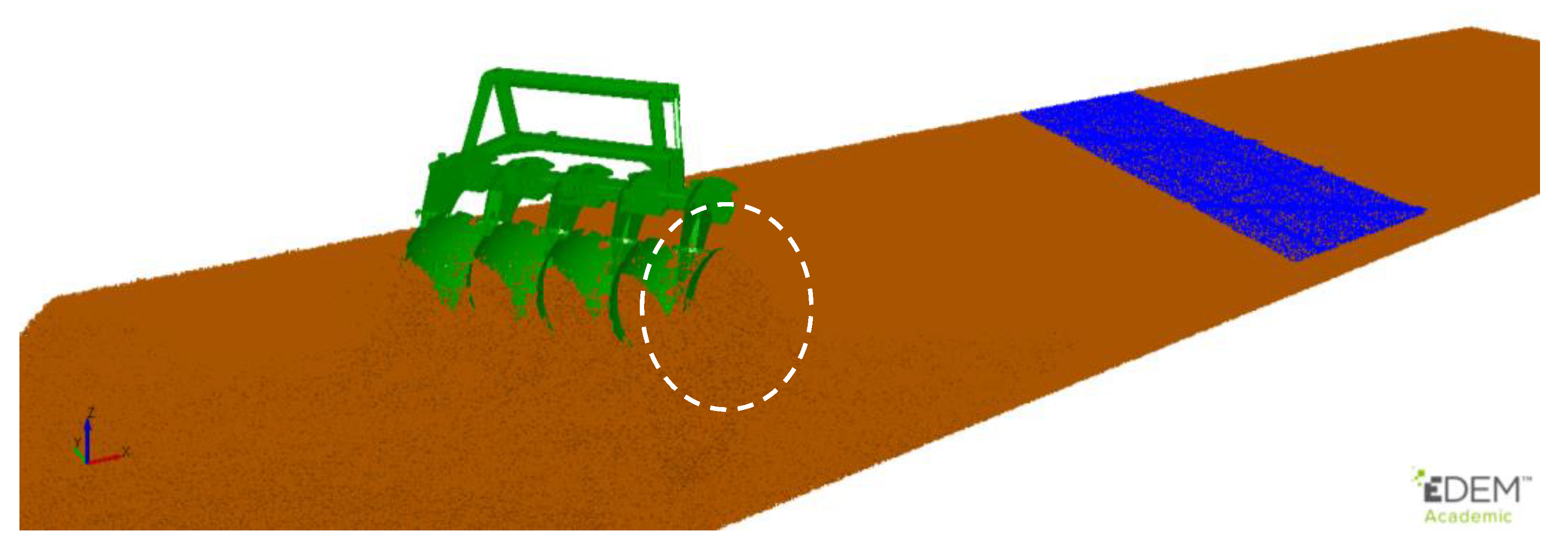
2.1. DEM and DEM-MBD Coupling Simulations

| Property | Value | Source |
|---|---|---|
| The density of sand particles (kg m−3) | 2600 | [20] |
| The density of steel (kg m−3) | 7865 | [21] |
| Shear modulus of soil (Pa) | 1 × 10⁷ | [22] |
| Shear modulus of steel (Pa) | 7.9 × 10¹⁰ | [21] |
| Poisson’s ratio of soil | 0.3 | [23] |
| Poisson’s ratio of steel | 0.3 | [24] |
| Yield strength of the soil (Pa) | 1.16 × 10⁶ | The default value in EDEM |
| Coefficient of friction (soil–soil) | 0.5 | Direct shear test |
| Coefficient of friction (soil–steel) | 0.5 | Direct shear test |
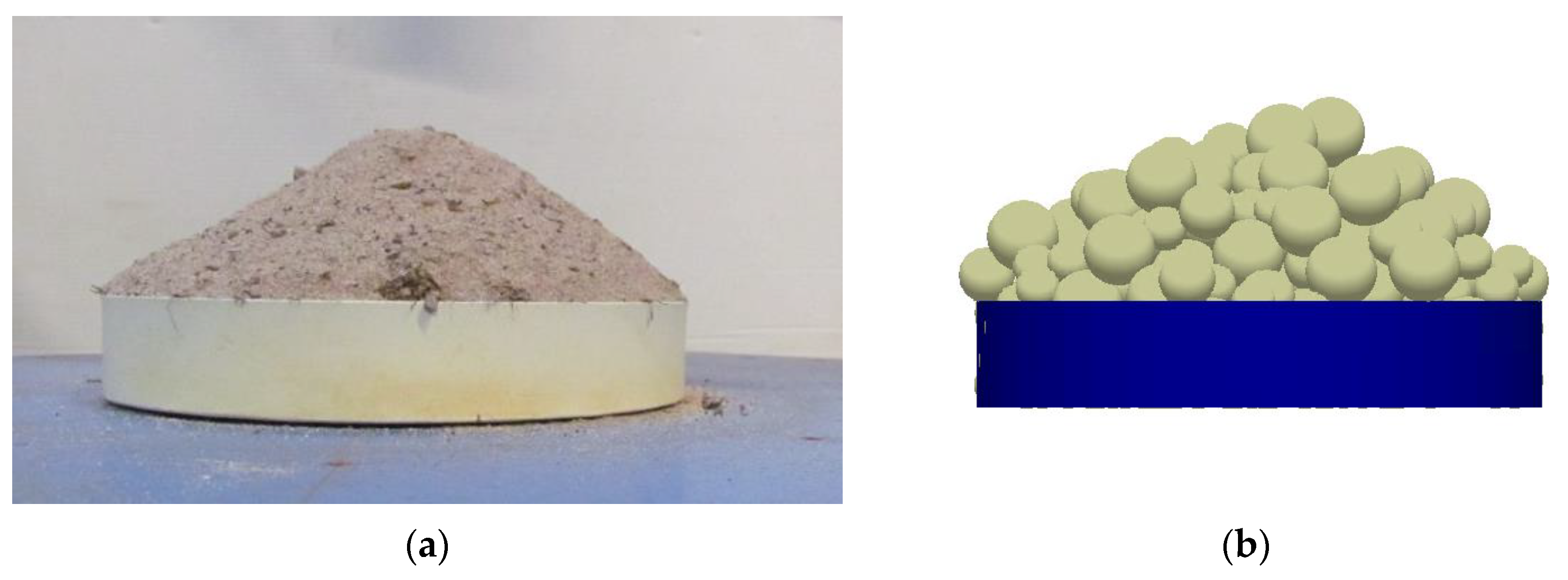
| Coefficient of rolling friction (soil–soil) | 0.15 | Calibrated by the angle of repose test |
| Coefficient of rolling friction (soil–steel) | 0.05 | Inclined surface test |
| Cohesive energy density between soil–soil (N m−2) | 2000 | Calibrated by the angle of the repose test |
| Particle size distribution | 0.5–2 | Selected based on the PSD of soil |
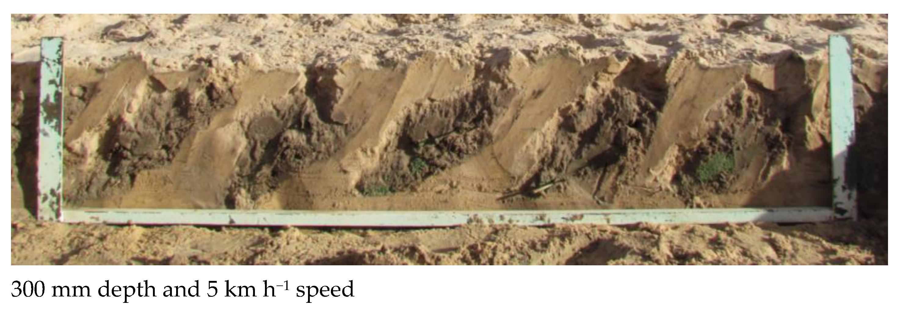
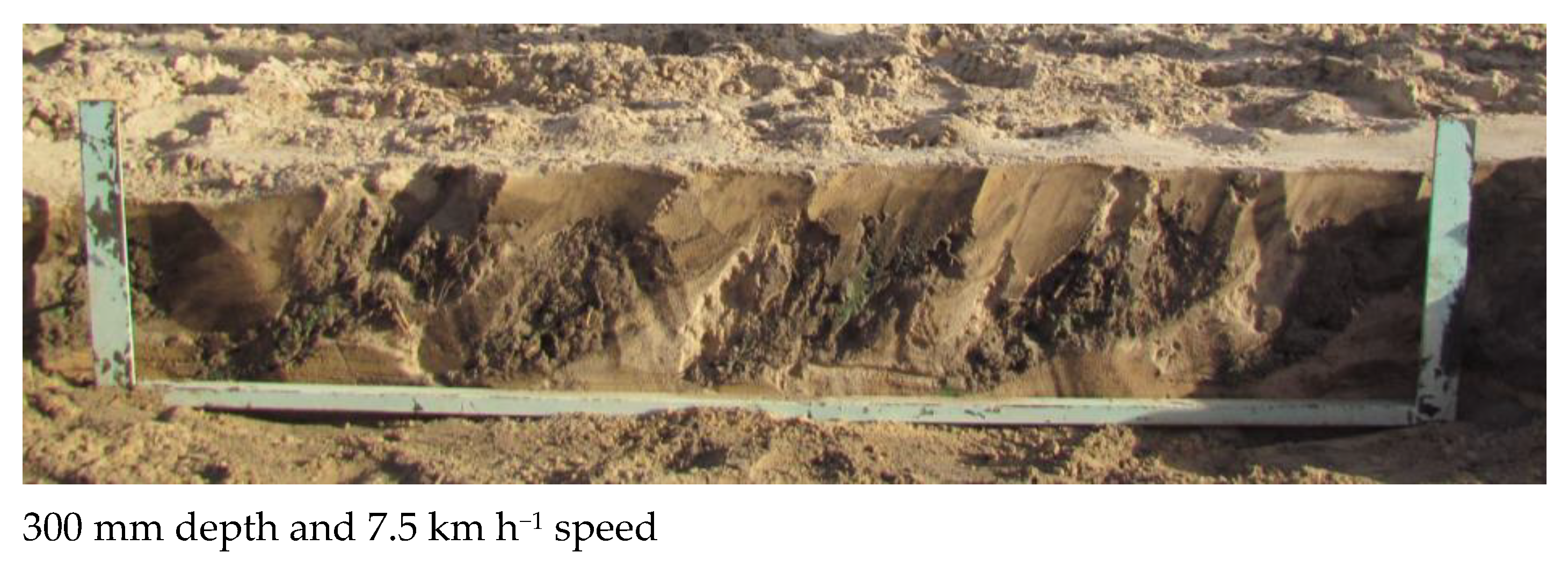
2.2. Field Tests
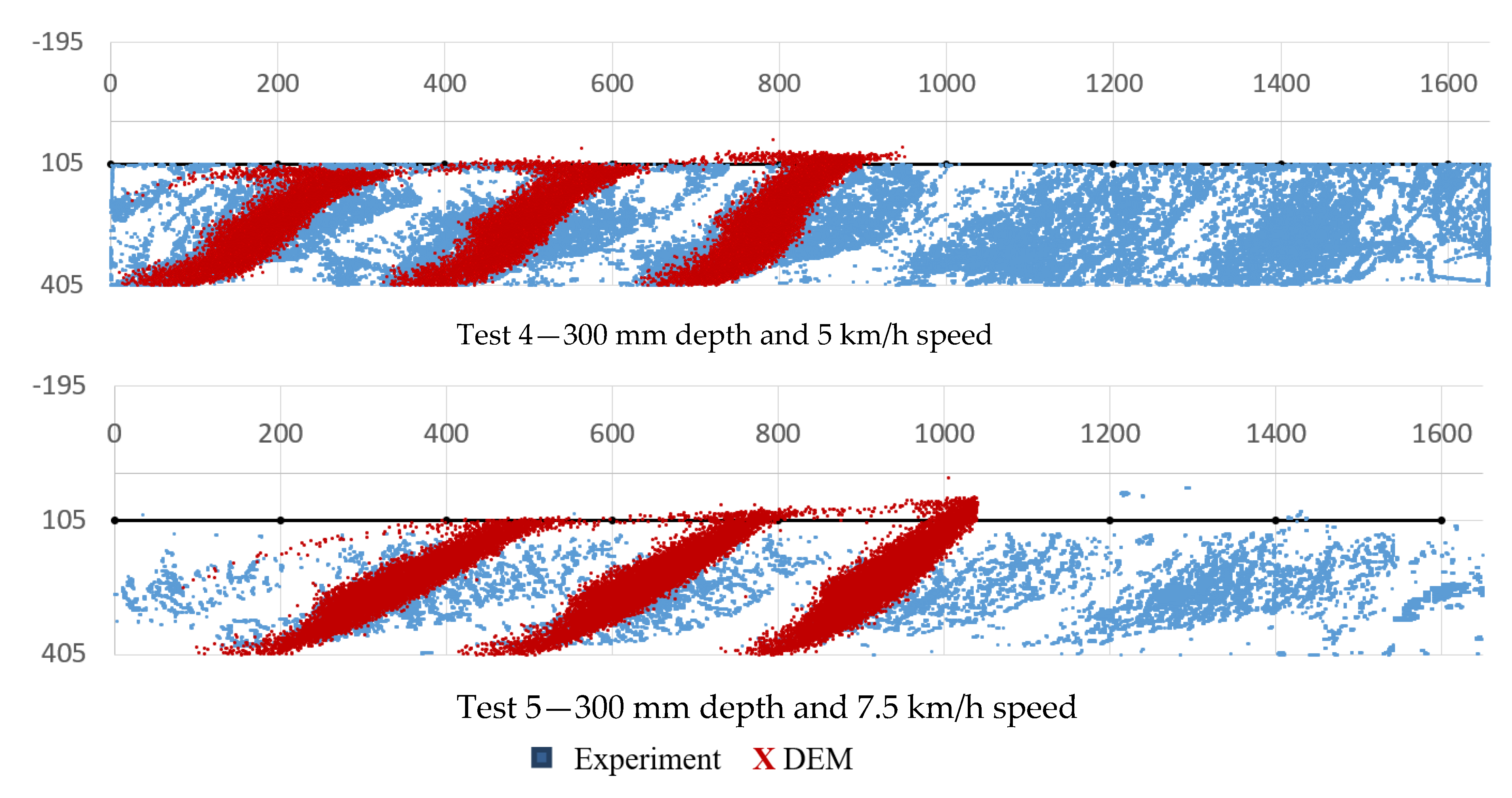
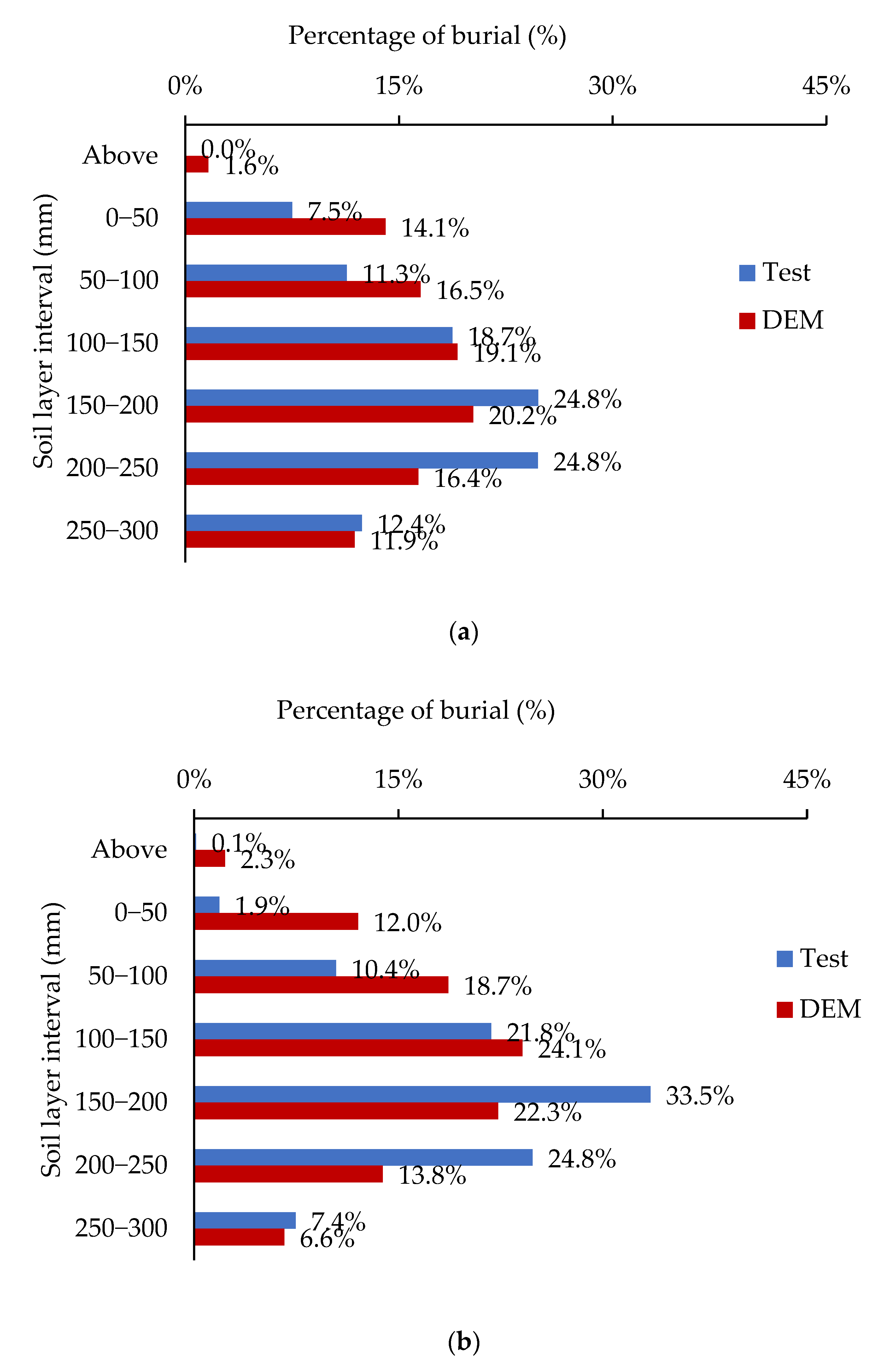
3. Results
4. Conclusions
Author Contributions
Funding
Institutional Review Board Statement
Data Availability Statement
Acknowledgments
Conflicts of Interest
Nomenclature
| a | Indices for sphere or implement |
| Ac | Contact area, (m2) |
| b | Indices for sphere or implement |
| e | Coefficient of restitution |
| Fc | Cohesion force, (N) |
| Fdn | Normal damping force, (N) |
| Fdt | Tangential damping force, (N) |
| Fn | Normal total contact force, (N) |
| Fsn | Normal contact force, (N) |
| Fst | Tangential contact force, (N) |
| Ft | Tangential total contact force, (N) |
| I | Moment of inertia, (kg m2) |
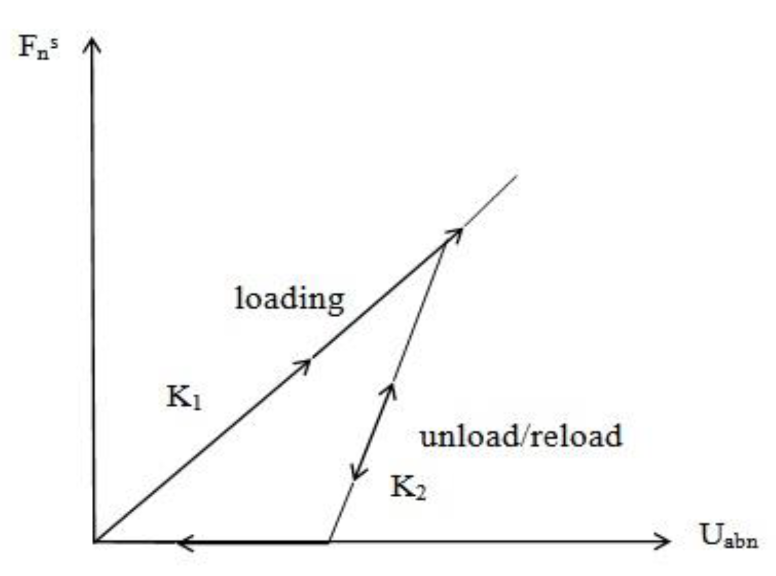
| K1 | Stiffness for loading, (N m−1) |
| K2 | Stiffness for unloading/reloading, (N m−1) |
| M | Moment, (N m) |
| Mr | Moment due to rolling friction, (N m) |
| m | Mass, (kg) |
| meq | Equivalent mass (kg) |
| nc | Damping factor |
| nk | Stiffness factor |
| r | Radius (m) |
| req | Equivalent radius, (m) |
| rcon | Perpendicular distance of contact point from the centre of mass, (m) |
| R | Rotational acceleration, (rad s−2) |
| Uabn | Normal component of the relative displacement, (m) |
| Uabt | Tangential component of the relative displacement, (m) |
| Ůabn | Normal component of the relative velocity, (m s−1) |
| Ůabt | Tangential component of the relative velocity, (m s−1) |
| U0 | Residual overlap, (m) |
| Ü | Translational acceleration, (m s−2) |
| Y | Yield strength (MPa) |
| Greek letters | |
| µ | Coefficient of friction |
| μr | Coefficient of rolling friction |
| λθ | Unit vector of angular velocity |
| ξ | Cohesion energy density (J m−3) |
References
- Nkakini, S.O. Draught force requirements of a disc plough at various tractor forward speeds in loamy sand soil during ploughing. Int. J. Adv. Res. Eng. Tech. 2015, 6, 52–68. [Google Scholar]
- Aybek, A.; Baser, E.; Arslan, S.; Ucgul, M. Determination of the effect of biodiesel use on power take-off performance characteristics of an agricultural tractor in a test laboratory. Turk. J. Agric. For. 2011, 35, 103–113. [Google Scholar] [CrossRef]
- Pratley, J.E.; Kirkegaard, J. (Eds.) Australian Agriculture in 2020: From Conservation to Automation; Agronomy Australia by Graham Centre for Agricultural Innovation; Charles Sturt University: Wagga Wagga NSW, Australia, 2019. [Google Scholar]
- Van Muysen Van Oost, W.K.; Govers, G. Soil translocation resulting from multiple passes of tillage under normal field operating conditions. Soil Tillage Res. 2006, 87, 218–230. [Google Scholar] [CrossRef]
- Li, S.; Lobb, D.; Lindstrom, M.J. Tillage translocation and tillage erosion in cereal-based production in Manitoba, Canada. Soil Tillage Res. 2007, 94, 164–182. [Google Scholar] [CrossRef]
- Plouffe, C.; Lague, C.; Tessier, S.; Richard, M.J.; McLaughlin, N.B. Moldboard plow performance in a clay soil: Simultaneous and experiment. Trans. ASAE 1999, 42, 1531–1539. [Google Scholar] [CrossRef]
- Aikins, K.A.; Antille, D.L.; Ucgul, M.; Barr, J.B.; Jensen, T.A.; Desbiolles, J.M. Analysis of effects of operating speed and depth on bentleg opener performance in cohesive soil using the discrete element method. Comput. Electron. Agric. 2021, 187, 106236. [Google Scholar] [CrossRef]
- Aikins, K.A.; Barr, J.B.; Antille, D.L.; Ucgul, M.; Jensen, T.A.; Desbiolles, J.M. Analysis of effect of bentleg opener geometry on performance in cohesive soil using the discrete element method. Biosyst. Eng. 2021, 209, 106–124. [Google Scholar] [CrossRef]
- Aikins, K.A.; Ucgul, M.; Barr, J.B.; Jensen, T.A.; Antille, D.L.; Desbiolles, J.M. Determination of discrete element model parameters for a cohesive soil and validation through narrow point opener performance analysis. Soil Tillage Res. 2021, 213, 105123. [Google Scholar] [CrossRef]
- Ucgul, M.; Saunders, C.; Fielke, J.M. A Method of quantifying discrete element method simulations of top soil burial from a mouldboard plough. In Proceedings of the 2016 ASABE Annual International Meeting, Orlando, FL, USA, 17–20 July 2016. [Google Scholar]
- Zeng, Z.; Ma, X.; Chen, Y.; Qi, L. Modelling residue incorporation of selected chisel ploughing tools using the discrete element method (DEM). Soil Tillage Res. 2020, 197, 104505. [Google Scholar] [CrossRef]
- Sadek, M.A.; Chen, Y.; Zeng, Z. Draft force prediction for a high-speed disc implement using discrete element modelling. Biosyst. Eng. 2021, 202, 133–141. [Google Scholar] [CrossRef]
- Fielke, J.M.; Ucgul, M.; Saunders, C. Discrete element modelling of soil-implement interaction considering soil plasticity, cohesion and adhesion. In 2013 Kansas City, Missouri, July 21–July 24, 2013; American Society of Agricultural and Biological Engineers: St. Joseph, MI, USA, 2013. [Google Scholar]
- EDEM. EDEM Theory Reference Guide; DEM Solutions Ltd.: Edinburgh, UK, 2011. [Google Scholar]
- Walton, O. Elastic-Plastic Contact Model; Company Report, DEM Solutions: Edinburgh, UK, 2006. [Google Scholar]
- Walton, O.R.; Braun, R.L. Stress calculations for assemblies of inelastic spheRes. in uniform shear. Acta Mech. 1986, 63, 73–86. [Google Scholar] [CrossRef]
- Raji, A.O. Discrete Element Modelling of the Deformation of Bulk Agricultural Particles. Ph.D. Thesis, University of Newcastle, Newcastle upon Tyne, UK, 1999. [Google Scholar]
- Li, P.; Ucgul, M.; Lee, S.H.; Saunders, C. A new approach for the automatic measurement of the angle of repose of granular materials with maximal least square using digital image processing. Comput. Electron. Agric. 2020, 172, 105356. [Google Scholar] [CrossRef]
- Li, P.; Lee, S.-.H.; Park, J.-S. Development of a global batch clustering with gradient descent and initial parameters in colour image classification. IET Image Process 2019, 13, 161–174. [Google Scholar] [CrossRef]
- Huser, A.; Kvernvold, O. Prediction of sand erosion in process and pipe components. In BHR Group Conference Series Publication; Mechanical Engineering Publications Limited: London, UK, 1998; Volume 31, pp. 217–228. [Google Scholar]
- Hudson Tool Steel. P20 Mold Steel. 2016. Available online: http://www.hudsontoolsteel.com/technical-data/steelP0 (accessed on 10 October 2022).
- Academia. Some Useful Numbers for Rocks and Soils. 2015. Available online: www.academia.edu/4056287/Some_Useful_Numbers_for_rocks_and_soils (accessed on 10 October 2022).
- Asaf, Z.; Rubinstein, D.; Shmulevich, I. Determination of discrete element model parameters required for soil tillage. Soil Tillage Res. 2007, 92, 227–242. [Google Scholar] [CrossRef]
- Budynas, R.G.; Nisbett, K.J. Shigley’s Mechanical Engineering Design; McGraw-Hill Education: New York, NY, USA, 2012. [Google Scholar]
- Li, P.; Ucgul, M.; Lee, S.H.; Saunders, C. A new method to analyse the soil movement during tillage operations using a novel digital image processing algorithm. Comput. Electron. Agric. 2019, 156, 43–50. [Google Scholar] [CrossRef]
- Ucgul, M.; Saunders, C.; Davies, S. Insights into One-Way Disc Ploughs. Available online: https://groundcover.grdc.com.au/innovation/precision-agriculture-and-machinery/insights-into-one-way-disc-ploughs (accessed on 20 October 2022).


| Sieve Size (mm) | Percentage Retained (%) |
|---|---|
| 2.36 | 7.2 |
| 1.18 | 10.6 |
| 0.6 | 20.2 |
| 0.3 | 39.0 |
| 0.15 | 19.6 |
| 0.075 | 3.2 |
| <0.075 | 0.2 |
Disclaimer/Publisher’s Note: The statements, opinions and data contained in all publications are solely those of the individual author(s) and contributor(s) and not of MDPI and/or the editor(s). MDPI and/or the editor(s) disclaim responsibility for any injury to people or property resulting from any ideas, methods, instructions or products referred to in the content. |
© 2023 by the author. Licensee MDPI, Basel, Switzerland. This article is an open access article distributed under the terms and conditions of the Creative Commons Attribution (CC BY) license (https://creativecommons.org/licenses/by/4.0/).
Share and Cite
Ucgul, M. Simulating Soil–Disc Plough Interaction Using Discrete Element Method–Multi-Body Dynamic Coupling. Agriculture 2023, 13, 305. https://doi.org/10.3390/agriculture13020305
Ucgul M. Simulating Soil–Disc Plough Interaction Using Discrete Element Method–Multi-Body Dynamic Coupling. Agriculture. 2023; 13(2):305. https://doi.org/10.3390/agriculture13020305
Chicago/Turabian StyleUcgul, Mustafa. 2023. "Simulating Soil–Disc Plough Interaction Using Discrete Element Method–Multi-Body Dynamic Coupling" Agriculture 13, no. 2: 305. https://doi.org/10.3390/agriculture13020305