Abstract
The appearance and meat quality of Penaeus vannamei are important indexes in the production process, and the quality of the product will be reduced if the defective shrimp is mixed in during processing. In order to solve this problem, a quality detection model of Penaeus vannamei based on deep learning was put forward. Firstly, the self-made dataset of Penaeus vannamei was expanded to enhance the generalization ability of the neural network. Secondly, the backbone of YOLOv5 (you only look once v5) is replaced by the lightweight network PP-LCNet that removes the dense layer at the end, which reduces the model parameters and calculation. Then, the 7 × 7 convolution DepthSepConv module is embedded in a PP-LCNet backbone, which effectively strengthens the feature extraction ability of the network. Ultimately, SiLU activation function is used to replace the Hardsigmoid and Hardswish activation functions in the PP-LCNet backbone to enhance the regularization ability and detection speed of the network. Through comparative experiments, the all-round performance of the Shrimp-YOLOv5s network is higher than the current mainstream classical model and the lightweight model. The mAP@0.5, mAP@0.5:0.95, detection speed, parameters, and calculation of Shrimp-YOLOv5s are 98.5%, 88.1%, 272.8 FPS (frames per second), 4.8 M, and 9.0 GFLOPs (giga floating point operations) respectively.
1. Introduction
Penaeus vannamei is one of the varieties of cultured shrimps with the highest output in the world. Its meat is firm and delicious, so it is very popular among consumers. In recent years, the annual output of Penaeus vannamei in China has hit record highs, with a national output of 1,815,600 tons in 2019 and 1,862,900 tons in 2020. In terms of the export scale of Penaeus vannamei, China ranks among the top five in the world [1], and Penaeus vannamei has already occupied a very important position in the aquatic industry of China. With the rise of the South American white shrimp industry, the number of processed products of South American white shrimp is increasing, and people’s requirements for product quality are becoming increasingly stringent [2]. In the process of fishing and transportation, Penaeus vannamei will experience mechanical damage such as squeezing and collision with objects such as fishing nets and transport containers, which will lead to the incompleteness or even death of shrimp bodies. Both kinds of defective shrimp are unqualified, which affects the quality of processed products and food safety [3,4]. At the same time, when the number of live shrimp in the transport container is too dense, many factors such as hypoxia, stress, and infectious diseases directly lead to the death of live shrimps [5]. The meat of dead Penaeus vannamei very easily rots and breeds bacteria, and when eaten by humans, it can cause gastrointestinal inflammation and even poisoning. According to national food safety requirements, these shrimp do not meet product quality safety standards [6]. Before shrimp is processed, some stale shrimp or incomplete shrimp are often mixed into it, which must be screened. However, this important link is usually completed by trained testing personnel, which requires high labor costs and has a limited accuracy. Therefore, it is of major significance to research methods of picking out the problem shrimp before processing. Yu et al. divided shrimp into two fresh grades according to volatile basic nitrogen (TVB-N) content, shrimp were divided into two fresh grades, and then the freshness of shrimp was classified by combining the stacked auto-encoders (SAE) algorithm and near-infrared hyperspectral imaging (HSI) technology. The accuracy of this method in calibration and prediction sets was 96.55% and 93.97% respectively [7]. In work by Liu et al. designed to distinguish soft-shelled shrimp from normal shrimp, the whole connection layer and convolution layer with poor performance in AlexNet network were removed, and a convolution layer splitting operation was added to the network. The network parameters were reduced, and the detection accuracy was improved, reaching 97.2% [8]. Aiming at the problem that the traditional shrimp recognition algorithm based on machine vision relies too much on feature setting, Hu et al. proposed an intelligent deep convolution neural network based on an improved LeNet-5 network. Two-layered CNN (convolutional neural network) and two-layered FC (fully connected) were used to reconstruct the LeNet-5 network to achieve efficient matching and recognition, and the final accuracy rate reached 96.84% [9]. Prema et al. put forward a hybrid SVM (support vector machines) and CNN model based on GAN (generative adversarial network), using a DCGANs(deep convolutional generative Adversarial Networks) enhancement algorithm to amplify the shrimp dataset. The findings demonstrated the model’s 98.1% accuracy rate for determining shrimps’ freshness [10]. Deep learning-based target identification technology is currently employed extensively across numerous industries; the YOLO (you only look once) series algorithm [11,12,13,14,15,16,17] is a significant part of target detection technology, and it is also widely used in food quality detection. Liu et al. improved the backbone structure of YOLOv3-tiny and introduced focusing loss, which improved the detection speed of damaged corn without decreasing the detection accuracy. The accuracy of the final model reached 89.8% [18]. Fahad et al. used deep learning target detection technology to detect the mold on food surface for the first time and found that the overall performance of YOLOv5 was superior to YOLOv4 and YOLOv3, with an average accuracy of 99.6% [19]. Wei et al. optimized a cherry dataset using a flood filling algorithm, which reduced the influence of environmental factors. After YOLOv5 network training, the accuracy of the final cherry-grading model reached 99.6% [20].
Although the traditional YOLO algorithm guarantees the model’s accuracy, it involves a lot of running parameters and calculations, making it difficult to deploy embedded devices and difficult to meet industrial requirements for detection speed. In order to solve these problems, a lightweight Penaeus vannamei quality detection model based on a YOLOv5s neural network was proposed, which not only kept the high detection accuracy of the model but also improved the detection speed and reduced the computational complexity of the model. This model takes into account the advantages of high detection accuracy, high speed, and low calculation cost and is suitable for embedded deployment and assembly line processing.
2. Materials and Methods
2.1. YOLOv5 Model
The overall layout of YOLOv5 is similar to that of YOLOv4, with the addition of a different CSP (cross stage partial) structure, focus structure, and CIOU (complete intersection over union) loss function. The diagram of YOLOv5s is shown in Figure 1, and its structure is divided into four sections: input, backbone, neck, and prediction.
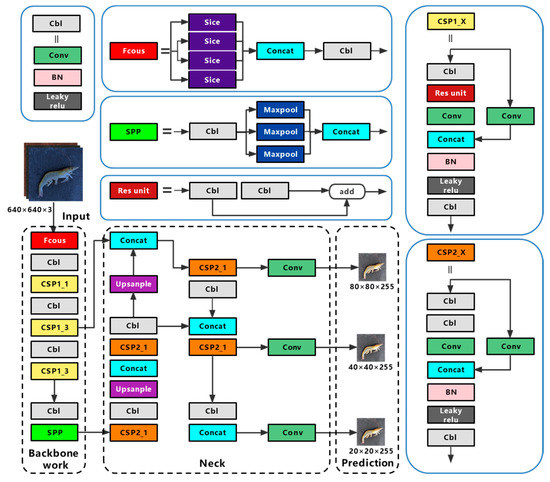
Figure 1.
The structure of YOLOv5s network. BN (Batch Normalization), SPP (spatial pyramid pooling), CSP (cross stage partial, CSP_1 with residual structure, CSP_2 without residual structure).
Mosaic data enhancement, auto learning bounding box anchors, and adaptive image scaling are used in the input. Mosaic data enhancement randomly scales, cuts, and arranges four images, and then puts them together into an image for training, which effectively improves the detection and recognition ability of the neural network for small targets. The auto learning bounding box automatically anchors the initial anchor box length and width value according to the anchor frame size of the dataset, compares it with the real anchor box in the training process, and iteratively updates the network parameters to gain the best anchor box value. The function of adaptive image reduction is to compress the input image size to the same standard size. Compared with traditional methods, adaptive image scaling of YOLOv5 reduces the part of the image that needs to be filled with black edges during the scaling process, reducing the amount of calculation in reasoning, and significantly improving the speed of network detection.
The backbone has structures such as focus, CSP and SPP (spatial pyramid pooling).The focus structure slices the image before it enters the backbone network, taking a value for an image every other pixel, and obtaining four similar images, before splicing them together to expand the RGB three channel by four times to 12 channels. Therefore, a binary down sampling feature map with complete information is produced. The CSP structure divides the feature information passed into the structure into two parts, some of which span convolution operation and are combined with the rest to reduce computational workload and maintain accuracy. A CPS 1_X structure with a residual component is applied to the backbone network, while a CPS 2_X structure with a normal volume integral is applied to the neck. The SPP structure model fixes the output size, which can process images of different sizes, prevent the over-fitting of training, and speed up training time.
The neck uses the FPN+PAN structure. FPN (feature pyramid network) is a top-down up sampling feature pyramid network structure, which integrates feature maps of various scales, because the upper layers of the network are deeper and contain more semantic information, which makes the semantic information of the bottom feature map richer. The PAN (path aggregation network) is a bottom-up down sampling feature pyramid network structure, which also fuses multiple scales of feature maps, as the lower layer has fewer convolutional layers and is able to obtain more feature localization information. The FPN and PAN structures complement each other by fusing each other’s processed feature maps, so that the output feature map has strong semantic features and strong positioning features.
The prediction uses NMS (non-maximum suppression) and CIOU loss. NMS classifies all rectangles into groups, calculates the best detection rectangle, and eliminates the remaining candidate rectangles. This is known as post-processing, and it improves the network’s detection performance. CIOU loss is a loss function, which takes the aspect ratio of the real boxes and the predicted frame as a penalty factor, making the regression of the target detection boxes more stable.
In the equation, represents the separation between the centroids of the real and predicted boxes. denotes the diagonal distance of the smallest outer rectangle C. denotes the parameter that measures the consistency of the aspect ratio of the two rectangular boxes. and indicate the true box width and height. and indicate the width and height of the prediction box.
2.2. Shrimp-Yolov5s Model
In this paper, a lightweight quality inspection model of Penaeus vannamei was proposed by combining YOLOv5s and PP-LCNet [21] network. The structure of the Shrimp-YOLOv5s network is shown in Figure 2, and its improvement mainly resides in the following three aspects.
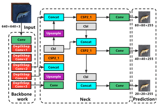
Figure 2.
Network structure diagram of Shrimp-YOLOv5s.
There are now three primary approaches for creating lightweight neural networks [22]: (A) Manual design of neural network structures for group convolution, depth-separable convolution, or other computationally efficient basic unit blocks for efficient stacking and sorting to build lightweight neural networks. (B) Neural architecture search using reinforcement learning, genetic algorithm, and other search strategies to search for the best performance of a given candidate neural network structure, so as to obtain a lightweight network. (C) Model compression, including model pruning, quantification, and knowledge refining: (a) pruning unimportant parts of the network structure; (b) converting the 32-bit floating-point parameters of the model into 8-bit integer operations; (c) transferring knowledge of the complex network structure to the simple network structure. Through the above methods, the purpose of reconstructing lightweight network structures can be achieved. In this paper, the lightweight network structure of PP-LCNet designed by hand is adopted.
In order to meet the requirements of specific scenarios with rigid requirements for inspection speed, such as industrial product quality inspection and mobile device side domains that need to balance accuracy, speed, and model size, academics have proposed lightweight architectures such as ShuffleNetV1, ShuffleNetV2, MobileNetV1, MobileNetV2, MobileNetV3, and GhostNet and other lightweight architectures, which guarantee good speed and accuracy while the models are lightweight. The lightweight high-performance network PP-LCNet offers a better balance of detection speed and accuracy for the same computational cost. PP-LCNet uses MobileNetV1′s DepthSepConv module containing depth-separable convolution to reconstruct the backbone network [23]. After removing the dense layer, the image input trunk passes through a conv layer, six 3 × 3 convolution DepthSepConv modules, and seven 5 × 5 convolution DepthSepConv modules in turn for feature extraction.
DepthSepConv module is a lightweight module containing depth-separable convolution and its structure is shown in Figure 3. Unlike other modules commonly used today, it does not have a residual structure for cross-region feature fusion, nor does it have concrete and add operations, which not only fail to improve model accuracy for small models but also slow down model inference. In this experiment, a 7 × 7 convolution DepthSepConv module was inserted between two 5 × 5 convolution DepthSepConv modules at the end of the backbone, and all three terminal modules have an SE attention mechanism. During training, the module inputs a 512 × 512 feature map to obtain a 1024 × 1024 feature map with enhanced features, and then the 5 × 5 convolution DepthSepConv module extracts features again and obtains a strong feature map of 512 × 512. The large convolution kernel effectively expands the receptive field while retaining and enhancing the high-level feature information, while the large-scale feature map magnifies the low-level feature information including the contour, edge, color, texture, and shape of the target, which effectively enhances the feature extraction ability of the network and improves the model performance [24].
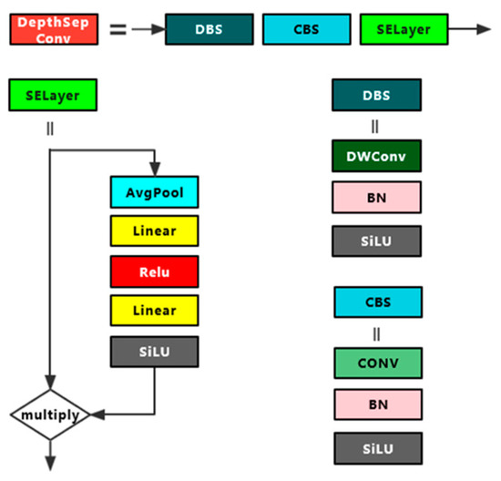
Figure 3.
DepthSepConv module structure diagram.
As shown in Figure 4, compared with normal convolution, deep separable convolution has the greatest advantage of being computationally inexpensive and efficient, and is therefore often used to build lightweight network structures. Deep separable convolution consists of depthwise convolution and pointwise convolution. The depthwise convolution has the same number of convolution kernels as the input feature map, and corresponds to each channel, such that each convolution kernel is only responsible for its own channel. The pointwise convolution uses 1 × 1 convolution kernels to sort out all the channel information of a single feature point extracted in the last step and subsequently increases the number of channels according to the output requirements [25].
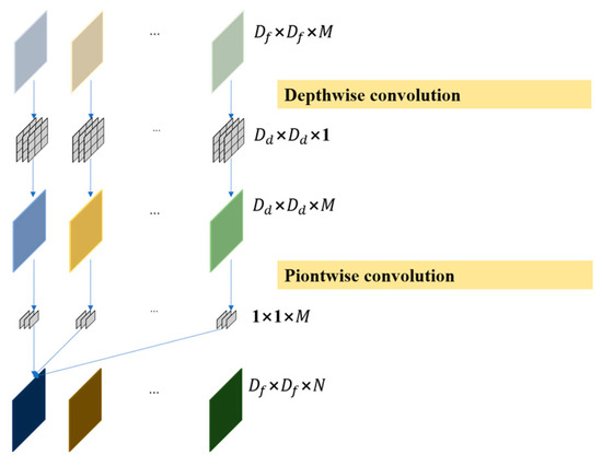
Figure 4.
Deep separable convolution schematic diagram.
In the equation, represents the size of the convolution kernel of depthwise convolution. represents the size of the input feature map. represents the number of convolution kernels for depthwise convolution and pointwise convolution. denote the number of channels for the input and output feature maps.
Neural networks fit various curves through nonlinear factors provided by activation functions. In artificial neural networks, it is very important to select appropriate activation functions. The Hardsigmoid and Hardswish nonlinear functions are widely used in PP-LCNet networks. Hardsigmoid and Hardswish use Relu6 to construct an approximate function of a sigmoid, which successfully reduces the calculation cost and improves the calculation efficiency, although its upper bound inhibition is prone to gradient saturation. At the same time, the optimization effect of these two activation functions in deep networks is not obvious, and it is difficult to balance accuracy and speed in a network with deep network layers. As shown in Table 1, when the backbone of YOLOv5 is replaced with PP-LCNet, the number of network layers reaches 328, and the number of network layers reaches 343 after adding a 7 × 7 convolution DepthSepConv module. At the same time, the newly added 7 × 7 convolution DepthSepConv module brings more parameters and calculation, but it also adds a burden to the task of filtering feature information. In order to solve the above problems, an SiLU activation function is used instead of these two functions, and its structure diagram is shown in Figure 5.

Table 1.
Comparison of number of layers, parameters, and calculation in the YOLOv5s improvement process.
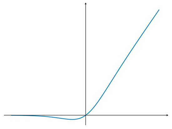
Figure 5.
SiLU activation function structure diagram.
The SiLU function is a special form of the Swish function [26,27], which has no upper bound or lower bound to avoid the gradient saturation problem, while having a strong regularization effect and the continued capacity to maintain the stability of the gradient update in networks with deeper layers. As shown in Figure 5, SiLU is a smooth function that is derivable everywhere and has continuous first and second order derivatives, which makes the network easier to train and can effectively speed up the network inference.
2.3. Dataset Preparation
In this experiment, a home-made dataset of Penaeus vannamei was created, and a total of 1575 images of white shrimp were collected, including 514 images of single normal shrimp, 439 images of single incomplete shrimp, 406 images of single stale shrimp, and 216 images of multiple mixed images wherein the images were mixed with 216 images. In order to enhance the generalization ability of the neural network and more closely recreate the processing practice, dataset collection should pay attention to the posture of the shrimp, the appearance of the defective shrimp, and the rotten degree of stale shrimp. As shown in Figure 6, the appearance defects of Penaeus vannamei include crushing, missing head, missing tail, and breaking. The TVB-N content of the stale shrimps was greater than 30 mg/100 g [28].
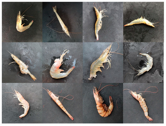
Figure 6.
Starting from the first row, the order is normal shrimp, incomplete shrimp, and stale shrimp.
In order to improve the learning ability of the network and to avoid overfitting the network due to an insufficient number of datasets, a Python program was used for data enhancement. Random rotation, image flipping, noise addition, blur, lighting transformations, zoom, and merge images were used to expand the data sample, and finally 10,201 images were obtained. Figure 7 gives an example of the enhanced Penaeus vannamei images. The labeling tool was used to set the categories of fresh, deficient, and stale shrimps to 0, 1, and 2, respectively, and the labels to normal, incomplete, and stale. The dataset was labelled to generate target information to be saved in a “.txt” file in YOLO data format. The Python program was used to rename data samples and the corresponding label files, disrupt the order of the datasets, and then randomly divide the training set, verification set, and test set with the ratio distribution of 8:1:1.
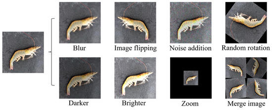
Figure 7.
Data enhancement.
2.4. Assessment Indicators
This experiment adopts the commonly used evaluation indexes for target detection. P (precision) and R (recall), FPS (frames per second), mAP (mean average precision), the model parameters, and FLOPs (floating point operations) are used as evaluation indexes to evaluate the model performance. Among them, the IOU (intersection over union) threshold for judging whether the prediction result is correct is greater than a certain value of mAP, such as 0.5, 0.6, 0.7, etc. The larger the threshold, the lower the accuracy. When the IOU threshold is 0.5 to 0.95, 10 values are taken at a step size of 0.05, and the value obtained by averaging them is referred to as mAP@0.5:0.95, while the average precision of the IOU threshold is mAP@0.5. The specific formula is as follows.
In the equation, TP (true positive) represents the number of targets with positive samples and positive predicted results. FP (false positive) represents the number of targets with another sample but where the prediction result is positive. FN (false negative) indicates the number of targets whose samples belong to the positive category but whose predicted results belong to another category. N (number) indicates the number of samples tested. T (time) denotes the time required to test the full sample.
3. Results and Discussion
3.1. Training Process
This training is based on the deep learning framework Pytorch, and the environment configuration and training parameters are shown in Table 2.
Table 2.
Experimental environment configuration and training parameters.
The neural network was trained by a training set and a verification set, and the quality detection model of Penaeus vannamei was obtained. Then, the test set was used to test the actual effectiveness and detection speed of the model.
From Figure 8, it can be seen that with the increase in the number of epochs, the training loss values gradually decreased: after 120 epochs, the model loss values were generally less than 0.02 and tended to level off. As shown in Table 3, after training, the precision of normal shrimp, incomplete shrimp, and stale shrimp iwa 96.8%, 93.9% and 95.1%, respectively, The rates of all precision and all recall were 95.8% and 95.2%, respectively, 98.5% for mAP@0.5, 88.1% for mAP@0.5:0.95, and the detection speed on a single RTX 2080 Ti graphics card was 272.8FPS. The accuracy and speed of the model training results can meet the requirements of factory assembly line processing.
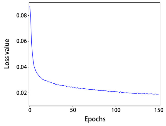
Figure 8.
Loss value curve.
Table 3.
The training results of the model include precision, recall, mAP@0.5, and mAP@0.5:0.95.
In the confusion matrix, the values on the main diagonal are the number of correctly predicted samples, and the values in other positions are the number of incorrectly predicted samples. On this basis, the confusion matrix of YOLOv5 adds the values of missed detection (background FN, the model recognizes the target as the background) and fake detection (background FP, the model recognizes the background as the target), which can test the model performance more comprehensively. The number of pictures in this test was 1011, which included 537 normal shrimp samples, 424 incomplete shrimp samples, and 381 stale shrimp samples. The experimental results are shown in Figure 9, the predicted correct numbers of normal shrimp, incomplete shrimp, and stale shrimp were 527, 395, and 357, the number of missed detections was 17, and the number of fake detections was 78. Although there were some missing and false detections in the test results, the accuracy of the model remained at a high level.
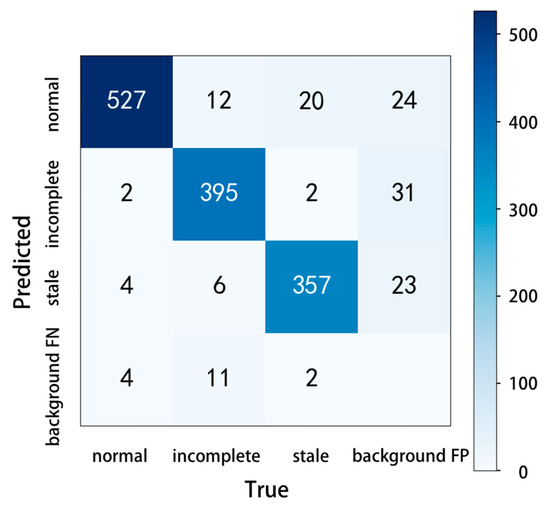
Figure 9.
Confusion matrix.
3.2. Ablation Experiments
In order to verify the detection effect of the pre-quality detection model of Penaeus vannamei, different improvement points based on a YOLOv5s neural network were trained and compared. The results of the experiment are shown in Figure 10 and Table 4. The YOLOv5s backbone network was first reconstructed and tested using the DepthSepConv module in the lightweight network PP-LCNet, and then the 7 × 7 convolutional kernel DepthSepConv module and the SiLU activation function were added and tested for network performance one by one, respectively. Constructing a PP-LCNet without terminal dense layers as the backbone of YOLOv5 can greatly reduce the parameters and calculation of the model and improve the detection speed of the model. The network model parameters were reduced by 45.8%, FLOPs was reduced by 49.7%, and the detection speed increased by 14 FPS, but mAP@0.5:0.95 and mAP@0.5 were also reduced by 1.8% and 0.9%, respectively. By replacing the other non-linear functions in the PP-LCNet backbone network with SiLU activation, the detection speed of the network model increased by 11.1 FPS, while other metrics remained largely unchanged. Inserting a 7 × 7 convolution kernel DepthSepConv module into the PP-LCNe backbone network can increase the network receptive field and feature extraction ability, and effectively improve the detection accuracy of the network model at the cost of a small amount of parameters and calculation. After adding the 7 × 7 convolution kernel DepthSepConv module, the model mAP@0.5:0.95 increased by 1.3% and mAP@0.5 increased by 0.6%. On the basis of inserting the 7 × 7 convolution kernel DepthSepConv module, using SiLU activation to replace other nonlinear functions in the backbone network, the mAP@0.5:0.95 increased by 1.2%, and the detection speed increased by 21.5 FPS. The 7 × 7 convolution kernel DepthSepConv module not only deepens the number of network layers (now the number of network layers reaches 343), but also brings more feature information. Compared with Hardsigmoid and Hardswish, the SiLU activation function has a stronger regularization ability in deep networks and can filter out useless or unimportant feature information, thus effectively improving model accuracy and running fluency. The improvement of the model has little fluctuation in accuracy. The analysis shows that the original model has a high accuracy, and the mAP@0.5 of the YOLOv5 network reached 98.6%, while that of the model that initially replaced the PP-LCNet backbone network reached 97.7%, which limits the improvement of accuracy to some extent.
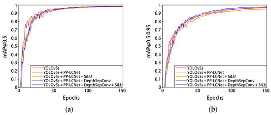
Figure 10.
Experimental results of each improved YOLOv5s model on the Penaeus vannamei dataset. (a) The change in curve in mAP@0.5; (b) the change in curve in mAP@0.5:0.95.
Table 4.
Improvement and comparison of YOLOv5s.
3.3. Comparison of Network
Figure 11 and Table 5 show the training results of this model and some mainstream classical network models on the self-built Penaeus vannamei dataset. Compared with YOLOv7-Tiny and YOLOX-Tiny, the network parameters and computational complexity of Shrimp-YOLOv5s were slightly lower, while the mAP@0.5:0.95 increased by 5.5% and 1.6%, respectively, mAP@0.5 increased by 1.1% and 2%, respectively, and the speed increased by 19.6 FPS and 64.5 FPS, respectively. Compared with the mainstream classical target detection algorithms SSD and Faster-RCNN, the parameters and calculation of Shrimp-YOLOv5s are greatly reduced, and the model accuracy and detection speed are significantly improved. Compared with the current mainstream classical target detection model and some lightweight improved models, Shrimp-YOLOv5s has a better overall performance. The improvement of Shrimp-YOLOv5s greatly reduces the calculation of the model parameters while ensuring the accuracy and speed of model detection, taking into account the performance and portability.
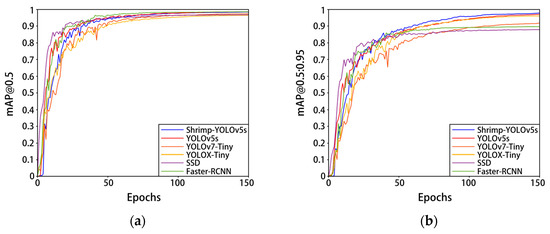
Figure 11.
Experimental results of different models on the Penaeus vannamei dataset. (a) The change in curve in mAP@0.5; (b) the change in curve in mAP@0.5:0.95.
Table 5.
Comparison of six models on dataset of Penaeus vannamei.
The results of the test are shown in Figure 12. The analysis shows that Shrimp-YOLOv5s has a lower rate of missed detections, false detections, and overlapping detections compared with other models. This is because the 7 × 7 convolutional DepthSepConv module in the backbone not only expands the perceptual field of the model but also enables the large size feature map, which enhances the ability of the model to identify features and thus reduces the missed and false detection rates. At the same time, the introduction of the SiLU activation function into the improved PP-LCNet backbone can improve the regularization ability of the model to better filter out some useless feature information, which can effectively suppress the detection overlap and false detection. Through comparative experiments, the comprehensive performance of the Shrimp-YOLOv5s network is higher than that of the current mainstream classic model and lightweight model.
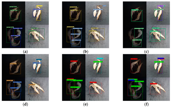
Figure 12.
Prediction results for several models. The results predicted by the following models are shown: (a) Shrimp-YOLOv5s; (b) YOLOv5s, including seven correct detections, one false detection, and one overlapping detection; (c) YOLOv7-Tiny, including five correct detections, one false detection, two missed detections, and one overlapping detection; (d) YOLOX-Tiny, including seven correct detections and two missed detections; (e) SSD, including six correct detections and two missed detections; (f) Faster-RCNN, including five correct predictions, two missed detections, and two overlapping detections.
4. Conclusions
The traditional artificial selection methods of Penaeus vannamei are subjective and inefficient; to address these problems, a lightweight improved neural network Shrimp-YOLOv5s is proposed. PP-LCNet is used to reconstruct the backbone of YOLOv5 and remove the dense layer at the end, so as to realize the lightweight nature of the model, greatly reducing the amount of model parameters and calculation. Inserting a 7 × 7 DepthSepConv module into the backbone network expands the network receptive field and feature extraction ability and effectively improves the detection accuracy of the model with a small amount of network parameters. At the same time, SiLU is used instead of the Hardsigmoid and Hardswish activation functions of the backbone network to alleviate the gradient saturation problem in deep network training, which can enhance the accuracy and reasoning speed of the model. The experiments conducted herein show that the improved method of Shrimp-YOLOv5s can reduce the calculation of the model, improve the detection speed, and ensure that the accuracy is not lost. Compared with YOLOv5s, the parameters of Shrimp-YOLOv5s are reduced by 32.4%, the calculation amount is reduced by 44.8%, the detection speed is increased by 14.6%, the mAP@0.5:0.95 is increased by 0.7%, and the mAP@0.5 is almost the same. Therefore, Shrimp-YOLOv5s has a good application prospect in processing quality detection of Penaeus vannamei.
Author Contributions
Y.C.: conceptualization, methodology, software, validation, writing—original draft preparation; X.H.: resources, supervision, funding acquisition, writing—review and editing; C.Z. and S.T.: investigation, formal analysis; N.Z. and W.X.: data curation, software, supervision. All authors have read and agreed to the published version of the manuscript.
Funding
This work was supported by the Fujian Engineering College School Marine Research Special Fund (GY-Z22062).
Institutional Review Board Statement
Not applicable.
Informed Consent Statement
Not applicable.
Data Availability Statement
The data collected in this research are available when required.
Conflicts of Interest
The authors declare no conflict of interest.
References
- Fishery Bureau of the Ministry of Agriculture (FBMA). China Fishery Statistical Yearbook; China Agriculture Publishing House (Chapter 2): Beijing, China, 2021. [Google Scholar]
- Yin, S.; Han, F.; Chen, M.; Li, K.; Li, Q. Chinese urban consumers’ preferences for white shrimp: Interactions between organic labels and traceable information. Aquaculture 2020, 521, 735047. [Google Scholar] [CrossRef]
- Kanduri, L.; Eckhardt, R.A. Food Safety in Shrimp Processing: A Handbook for Shrimp Processors, Importers, Exporters and Retailers; John Wiley & Sons: Hoboken, NJ, USA, 2008. [Google Scholar]
- Hannan, M.A.; Habib, K.A.; Shahabuddin, A.M.; Haque, M.A.; Munir, M.B. Processing of Shrimp. In Post-Harvest Processing, Packaging and Inspection of Frozen Shrimp: A Practical Guide; Springer: Singapore, 2022; pp. 60–61. [Google Scholar]
- Fotedar, S.; Evans, L.H. Health management during handling and live transport of crustaceans: A review. J. Invertebr. Pathol. 2011, 106, 143–152. [Google Scholar] [CrossRef] [PubMed]
- NY/T 840-2020; Green Food Shrimp. The National Agriculture Ministry: Beijing, China, 2020.
- Yu, X.; Tang, L.; Wu, X.; Lu, H. Nondestructive Freshness Discriminating of Shrimp Using Visible/Near-Infrared Hyperspectral Imaging Technique and Deep Learning Algorithm. Food Anal. Methods 2018, 11, 768–780. [Google Scholar] [CrossRef]
- Liu, Z.; Jia, X.; Xu, X. Study of shrimp recognition methods using smart networks. Comput. Electron. Agric. 2019, 165, 104926. [Google Scholar] [CrossRef]
- Hu, W.C.; Wu, H.T.; Zhang, Y.F.; Zhang, S.H.; Lo, C.H. Shrimp recognition using ShrimpNet based on convolutional neural network. J. Ambient. Intell. Humaniz. Comput. 2020, 1–8. [Google Scholar] [CrossRef]
- Prema, K.; Visumathi, J. An Improved Non-Destructive Shrimp Freshness Detection Method Based on Hybrid CNN and SVM with GAN Augmentation. In Proceedings of the International Conference on Advances in Computing, Communication and Applied Informatics (ACCAI), Chennai, India, 28–29 January 2022; pp. 1–7. [Google Scholar]
- Redmon, J.; Divvala, S.; Girshick, R.; Farhadi, A. You Only Look Once: Unified, Real-Time Object Detection. In Proceedings of the IEEE Conference on Computer Vision and Pattern Recognition (CVPR), Las Vegas, NV, USA, 27–30 June 2016; pp. 779–788. [Google Scholar]
- Redmon, J.; Farhadi, A. YOLO9000: Better, Faster, Stronger. In Proceedings of the IEEE Conference on Computer Vision and Pattern Recognition (CVPR), Honolulu, HI, USA, 21–26 July 2017; pp. 6517–6525. [Google Scholar]
- Joseph, R.; Ali, F. YOLOv3: An Incremental Improvement. arXiv 2018, arXiv:1804.02767. [Google Scholar]
- Bochkovskiy, A.; Wang, C.; Liao, H. YOLOv4: Optimal Speed and Accuracy of Object Detection. arXiv 2020, arXiv:2004.10934. [Google Scholar]
- Jocher, G. YOLOv5. Available online: https://github.com/ultralytics/yolov5 (accessed on 1 November 2021).
- Li, C.; Li, L.; Jiang, H.; Weng, K.; Geng, Y.; Li, L.; Ke, Z.; Li, Q.; Cheng, M.; Nie, W.; et al. YOLOv6: A Single-Stage Object Detection Framework for Industrial Applications. arXiv 2022, arXiv:2209.02976. [Google Scholar]
- Wang, C.; Bochkovskiy, A.; Liao, H. YOLOv7: Trainable bag-of-freebies sets new state-of-the-art for real-time object detectors. arXiv 2022, arXiv:2207.02696. [Google Scholar]
- Liu, Z.; Wang, S. Broken Corn Detection Based on an Adjusted YOLO With Focal Loss. IEEE Access 2019, 7, 68281–68289. [Google Scholar] [CrossRef]
- Jubayer, F.; Soeb, J.A.; Mojumder, A.N.; Paul, M.K.; Barua, P.; Kayshar, S.; Akter, S.S.; Rahman, M.; Islam, A. Detection of mold on the food surface using YOLOv5. Curr. Res. Food Sci. 2021, 4, 724–728. [Google Scholar] [CrossRef] [PubMed]
- Han, W.; Jiang, F.; Zhu, Z. Detection of Cherry Quality Using YOLOV5 Model Based on Flood Filling Algorithm. Foods 2022, 11, 1127. [Google Scholar] [CrossRef] [PubMed]
- Cui, C.; Gao, T.; Wei, S.; Du, Y.; Guo, R.; Dong, S.; Lu, B.; Zhou, Y.; Lv, X.; Liu, Q.; et al. PP-LCNet: A Lightweight CPU Convolutional Neural Network. arXiv 2021, arXiv:2109.15099. [Google Scholar]
- Ge, D.H.; Li, H.; Zhang, L.; Liu, R.; Shen, P.; Miao, Q.G. Survey of Lightweight Neural Network. J. Softw. 2020, 31, 2627–2653. (In Chinese) [Google Scholar]
- Howard, A.G.; Zhu, M.; Chen, B.; Kalenichenko, D.; Wang, W.; Weyand, T.; Andreetto, M.; Adam, H. Mobilenets: Efficient convolutional neural networks for mobile vision applications. arXiv 2017, arXiv:1704.04861. [Google Scholar]
- Ding, X.; Zhang, X.; Han, J.; Ding, G. Scaling Up Your Kernels to 31 × 31: Revisiting Large Kernel Design in CNNs. In Proceedings of the IEEE Conference on Computer Vision and Pattern Recognition (CVPR), New Orleans, LA, USA, 18–24 June 2022; pp. 11953–11965. [Google Scholar]
- Chollet, F. Xception: Deep Learning with Depthwise Separable Convolutions. In Proceedings of the IEEE Conference on Computer Vision and Pattern Recognition (CVPR), Honolulu, HI, USA, 21–26 July 2017; pp. 1800–1807. [Google Scholar]
- Elfwing, S.; Uchibe, E.; Doya, K. Sigmoid-weighted linear units for neural network function approximation in reinforcement learning. Neural Netw. 2018, 107, 3–11. [Google Scholar] [CrossRef] [PubMed]
- Ramachandran, P.; Zoph, B.; Le, Q.V. Searching for activation functions. arXiv 2017, arXiv:1710.05941. [Google Scholar]
- GB 2733-2015; Hygienic Standard for Fresh and Frozenmarine Products of Animal Origin. The National Hygiene Ministry: Beijing, China, 2015.
- Ge, Z.; Liu, S.; Wang, F.; Li, Z.; Sun, J. Yolox: Exceeding yolo series in 2021. arXiv 2021, arXiv:2107.08430. [Google Scholar]
- Liu, W.; Anguelov, D.; Erhan, D.; Szegedy, C.; Reed, S.; Fu, C.Y.; Berg, A.C. SSD: Single Shot MultiBox Detector. In Proceedings of the Computer Vision—ECCV 2016; Lecture Notes in Computer Science; Springer: Cham, Switzerland, 2016; p. 9905. [Google Scholar]
- Ren, S.; He, K.; Girshick, R.; Sun, J. Faster R-CNN: Towards Real-Time Object Detection with Region Proposal Networks. arXiv 2015, arXiv:1506.01497. [Google Scholar] [CrossRef] [PubMed]


Disclaimer/Publisher’s Note: The statements, opinions and data contained in all publications are solely those of the individual author(s) and contributor(s) and not of MDPI and/or the editor(s). MDPI and/or the editor(s) disclaim responsibility for any injury to people or property resulting from any ideas, methods, instructions or products referred to in the content. |
© 2023 by the authors. Licensee MDPI, Basel, Switzerland. This article is an open access article distributed under the terms and conditions of the Creative Commons Attribution (CC BY) license (https://creativecommons.org/licenses/by/4.0/).