Abstract
We train and compare the performance of two different machine learning algorithms to learn changes in winter wheat production for fields from the southwest of Sweden. As input to these algorithms, we use cloud-penetrating Sentinel-1 polarimetry radar data together with respective field topography and local weather over four different years. We note that all of the input data were freely available. During training, we used information on winter wheat production over the fields of interest which was available from participating farmers. The two machine learning models we trained are the Light Gradient-Boosting Machine and a Feed-forward Neural Network. Our results show that Sentinel-1 data contain valuable information which can be used for training to predict winter wheat yield once two important steps are taken: performing a critical transformation of each pixel in the images to align it to the training data and then following up with despeckling treatment. Using this approach, we were able to achieve a top root mean square error of 0.75 tons per hectare and a top accuracy of 86% using a k-fold method with . More importantly, however, we established that Sentinel-1 data alone are sufficient to predict yield with an average root mean square error of 0.89 tons per hectare, making this method feasible to employ worldwide.
1. Introduction
Precision agriculture is the practice of using science and technology to improve farming in order to achieve the best outcome possible. More specifically, this means that we want to maximize yield while sustaining the long-term health of the soil and incurring the smallest possible impact on the environment. In particular, this is performed by using technology to collect information about the local variations within fields to adapt the use of fertilizers, seeds, crop nutrients, plant protection, and much more [1].
Most modern precision agriculture practices can be divided into the following three phases [2]: (a) data collection, (b) data analysis, and (c) operational application. Data collection can include collecting soil samples for analyses or using unmanned aerial vehicles (UAVs) such as drones or satellites with remote sensing devices. Modern farming machinery, such as combine harvesters, also contribute by collecting data about local variations in yield. Analysis, the second phase, commonly consists of employing mathematical models or machine learning models. The work detailed in this article mainly contributes to this phase of precision agriculture. The third phase, operational application, consists of using the obtained knowledge in order to improve yield, minimize environmental impact, or simply save money.
One approach in crop yield forecasting is to create some type of crop growth model. A crop growth model provides a relationship between a crop and its environment. Such a model is mostly used to estimate crop yield from physiological processes, such as crop management, weather, soil, etc., taking place in the surrounding crop environment. Typically crop growth models are developed based on simulations of important crop characteristics such as the leaf area index (LAI) as well as the evapotranspiration (ET) or the fraction of absorbed photosynthetically active radiation (fAPAR). LAI is directly linked to crop canopy development which naturally affects light interception and photosynthesis, while ET reflects the available water to support crop growth. Furthermore, fARAR indicates the fraction of photosynthetically active radiation absorbed by the canopy. The importance of fARAR lies in the fact that it is able to quantify the amount of energy that a crop receives from sunlight, which is a key factor for photosynthesis and, ultimately, crop growth [3]. In a review study of agricultural practices in [4], the authors describe that a “major limitation of crop growth models is the lack of spatial information on the actual conditions of each field or region”. A more extensive list of shortcomings is provided in [5], where the authors state that “the main limitations of crop growth models are the cost of obtaining the necessary input data to run the model, the lack of spatial information”, and “the input data quality”.
In many locations, such as the one in our study in southwest Sweden, optical sensors are not useful since cloud coverage is persistent through large parts of the crop growing season. Instead, synthetic aperture radar (SAR) has some advantages over optical sensors since they are not affected by atmospheric conditions and can therefore monitor the status of crops not only during the day but even during the night. Furthermore, SAR sensors can even penetrate canopies [3]. Such sensors do not suffer from the well-known saturation phenomenon of optical sensors when crops such as winter wheat reach medium to high canopy cover. It has been shown [3,4,5,6], for instance, that LAI and biomass could be estimated at medium to high canopy cover from such sensors since they have strong penetration capabilities. This was another reason we examined SAR as an input in our study for winter wheat yield.
Our effort in this work will not be to directly model quantities such as LAI, ET, or fARAR, which has been performed before in many studies, but instead examine whether it is possible for the proposed machine learning methods to fit a full end-to-end model in order to ascertain crop yield directly. We, therefore, bypass the crop growth model.
We will specifically investigate the possibilities of using two different ML models to predict winter wheat harvest on fields in the region of Skåne, in southwest Sweden, mainly with radar backscatter data from Sentinel-1 satellites. The two machine learning models we trained are the Light Gradient-Boosting Machine and a Feed-forward Neural Network.
Based on this main goal, several research questions are considered, such as (a) is there valuable information within Sentinel data in order for the ML model to accurately forecast harvests, (b) is there a benefit in including Sentinel-1 indices [7,8] as input data, and (c) can supplemental data such as weather, topology classification, and elevation affect the performance?
As input, we mainly use Sentinel-1 radar backscatter data. We furthermore also test how progressively extending these data with weather, topology classification of the terrain, and/or elevation can improve the resulting harvest forecasting accuracy. In order to ascertain accuracy but also to be able to train our ML algorithms, we collected harvest data for winter wheat fields in Skane, Sweden, during the years 2017, 2018, 2019, and 2020. We evaluate our results under a number of performance measures, such as the root mean square error, accuracy, and F1-score.
The paper is organized as follows. We begin by describing the state of the art in Section 2. This is then followed by Section 3, where data processing and methods employed are explained. This section also includes information about the filtering of speckle noise introduced by the Sentinel-1 satellite. Furthermore, information about harvest and auxiliary data can be found in Section 3.4 and Section 3.5. These sections are then followed by the Results Section 4 and, finally, the Discussion and Conclusions Section 5 and Section 6, respectively.
2. State of the Art and Challenges
The Sentinel-1 mission consists of two (Sentinel-1B, one of the twin satellites, has been out of service since December 2021 due to a power supply malfunction and, therefore, data may be limited after this date) polar-orbiting satellites [9] which are part of the Copernicus initiative of the European Radar Observatory. The polar orbit of the satellites results in higher revisit frequencies further away from the equator. The satellites are to operate day and night to enable imaging of the Earth’s surface, regardless of weather, through the use of a C-band Synthetic Aperture Radar (SAR) [10].
Sentinel-1 data are available as level-0, level-1, or level-2 products. Level-0 products are based on the raw signals received directly from the satellite. Level-1 products are produced from the level-0 products through the satellite instrument processing facility into Ground Range Detected (GRD) or Single Look Complex (SLC) byproducts. Most users make use of such level-1 products. We chose the level-1 GRD byproducts in this study mainly due to the fact that they can reduce the impact of speckle noise [9] in the data, as we describe in more detail later in Section 3.
It has been shown [11] that continuous monitoring of the development of the phenological stages, such as emergence, closure, and height, is possible through GRD Sentinel-1 data for several crops such as sugar beet, potato, maize, wheat, and English ryegrass. Comparing the time series of the radar backscatter with hydrometeorological data and field measurements, it was shown in [11] that data from Sentinel-1 do capture information about biomass changes and moisture (including to use the VH/VV ratio to reduce the influence of soil moisture). The VH/VV ratio is sensitive on an agriculture operative level to the increase in fresh biomass during the plant growth stages and to the decrease during senescence as the water content decreases.
Many studies [5,6] have successfully shown that, indeed, SAR-type data can be used to reliably monitor important parameters determining growth in crops. Recently, ref. [3] showed how LAI, for instance, can be reliably estimated from SAR images in order to produce a crop model for rice yield estimation. These SAR images were obtained from the COSMO-Sky-Med satellite. For example, in the case of sugar beet [5], radar data can be used to monitor the emergence and closure of the canopy, as well as estimate the crop height and biomass throughout the growing season. Similarly, for potato crops [4], radar data can be used to monitor canopy closure, as well as detect changes in biomass and moisture content. For maize and wheat, radar data can be used to monitor crop growth and development, as well as estimate biomass and yield. In the case of English ryegrass [5], radar data can be used to estimate grass height and biomass. Specifically, for winter wheat in the Netherlands, [11] could closely match all phenological stages: tillering, stem elongation, booting, heading, flowering, fruit development, ripening, and harvesting, to Sentinel-1 VV and VH backscatter data.
The ability to use Sentinel-1 data to detect important winter wheat phenological phases, including monitor yield, was also investigated in a study from Lebanon [12]. Temporal variations of the Sentinel-1 backscatter were analyzed as a function of phenological phases (germination, heading, and soft dough) and harvesting dates. It was shown there that the variations of the Sentinel-1 data could be used to estimate the dates of these important phases. The authors also investigated how the different polarization (VH, VV) and the ratio VV/VH with different incidence angles could be used to predict the important dates. These results also strengthened the findings in [7,8], which showed that the VH/VV ratio is important in accessing soil moisture. Works [13,14] discuss the importance of correctly handling the variations in Sentinel-1 incident angles for any Radiative Transfer (RT)-based model. Similarly, Refs. [15,16] studied the possibilities of using a temporal profile and regression analysis of Sentinel-1 data to continuously monitor the phenological development of barley and wheat.
In a relevant study from the region of Skåne in Sweden, Sentinel-2 satellite imagery was combined with local weather data, national soil databases, and local farmer data to train a Light Gradient Boosting Machine to predict winter wheat yield with an accuracy of 82% [17]. Other metrics for regression were also reported by the authors. However, these were used for training and not testing the models. As a result, their findings are not comparable with the results we present here, which come exclusively from testing against new data. Furthermore, the authors present one downside of using Sentinel-2 optical imagery—its dependence on cloud-free conditions to not block the imagery.
3. Data Processing and Methods
Sentinel-1 is a radar imaging satellite that can provide information about the Earth’s surface regardless of weather conditions or daylight. This makes it an ideal tool for monitoring agricultural crops over time. The radar signal emitted by Sentinel-1 interacts with the crops and provides information about their physical characteristics, such as height and structure. This information can be used to monitor the growth and development of crops throughout the season, allowing farmers and agronomists to make informed decisions about irrigation, fertilization, and pest management. With Sentinel-1 data, it is possible to measure the backscatter, or the amount of radar energy reflected back to the satellite from the Earth’s surface. This backscatter signal can be used to derive several biophysical parameters related to vegetation, such as vegetation water content, biomass, and vegetation height.
Specifically, the Sentinel-1 satellites use a single C-band SAR instrument operating with a center frequency of 5.405 GHz and dual polarization [10]. C-band radar is radar using the frequency ranges of 4.0 to 8.0 GHz, and is the portion of the electromagnetic spectrum allocated for commercial telecommunications via satellites, designated by the Institute of Electrical and Electronics Engineers (IEEE) [18]. SAR is an imaging radar commonly found on moving platforms, such as aircraft or satellites, which is able to produce high-resolution imagery with relatively small physical antennas. SAR works by transmitting a series of microwave signals and recording the backscatter from the Earth’s surface [19]. Normally, to achieve high-resolution imagery, a large aperture antenna is required for stationary radars. However, with a small moving antenna, successively recorded radar echoes may be processed and combined, giving the effect of a larger synthetic antenna aperture (hence the name) [18]. An advantage of SAR radar compared to optical imagery is the ability to operate regardless of weather conditions. Satellites using optical imagery are greatly impaired by clouds covering the target area [17]. The polarization of the radar can be horizontal (H) or vertical (V), and relates to the polarization of the transmitted or received signal. Different targets on the Earth’s surface have distinct polarization signatures. The signatures reflect each polarization with different intensities of the target. For example, forest canopy backscatters have different polarization properties than sea surface backscatters [10].
Sentinel-1 satellites have four acquisition modes, with Interferometric Wide (IW) swath being the main acquisition mode over land and three different product levels, with Level-1 being the most commonly used for end users [10]. IW mode supports VH and VV polarization with the highest resolution of 10.0 m [9]. However, the best resolution we managed to download from Sentinel Hub was 11.0 m. According to ESA, IW swath is the recommended main operational mode, as it avoids conflicts, preserves revisit performance, decreases operational costs, and builds up a consistent long-term archive of data [10]. We used the Ground Range Detected (GRD) product, which contains the detected amplitude from the SAR data and uses a multi-look feature to reduce the impact of speckling.
Additional processing of the Level-1 product, such as orthorectification and radiometric calibration (Figure 1), is needed for the SAR data to be able to measure true distance in the imagery and to convert digital numbers into physical units [20]. Undergoing orthorectification will allow us to correct images for topographic relief, camera tilt, and lens distortion. Furthermore, a Digital Elevation Model is used as a 3D representation of the terrain’s surface [9]. The result is imagery that can measure true distances.
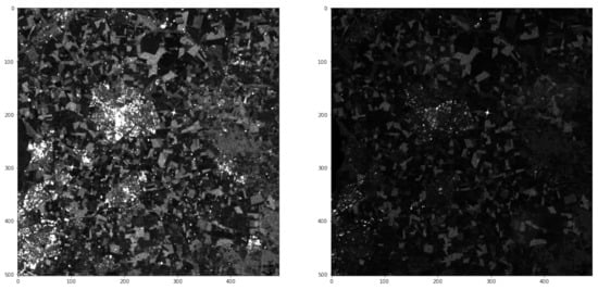
Figure 1.
Typical level-1 SAR backscatter, VH (left), and VV polarization (right), with orthorectification and radiometric calibration.
Since Sentinel-1 operates in the C-band radio waves from other applications, e.g., missile guidance can interfere with the originally transmitted signal from the satellite, causing radio frequency interference (RFI) [19]. An example of how RFI typically looks in the resulting backscatter can be seen in Figure 2. Some regions had particular issues with RFI, with up to ∼30% of images being distorted. Separating the part of the backscatter with RFI can be difficult, due to the values not being NaN or infinity. Instead, we employ the Sentinel-1 toolbox [10], where the data will be annotated with a flag at the source if they contain RFI, which we then identify and remove using the eo-learn python package.
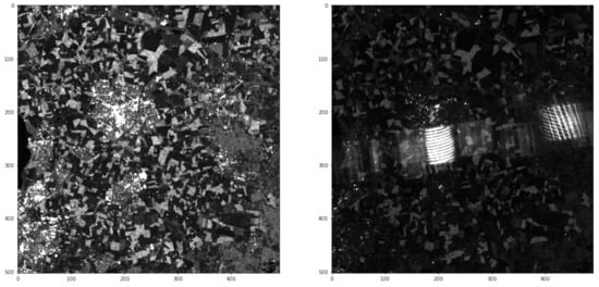
Figure 2.
An example of Sentinel-1 data altered by RFI. VV band (left) is not influenced. VV band (right), however, is heavily affected by RFI.
3.1. Study Area
The area of study was the region of Skåne in the southwest of Sweden (Figure 3), where a number of fields participating in this study cultivating winter wheat are located. The number of winter wheat fields from which the ground truth yield data were gathered was 49, 31, 132, and 88 for the years 2017, 2018, 2019, and 2020, respectively. The distribution of field sizes had a mean of 20 Hectares and a median of 14 Hectares.
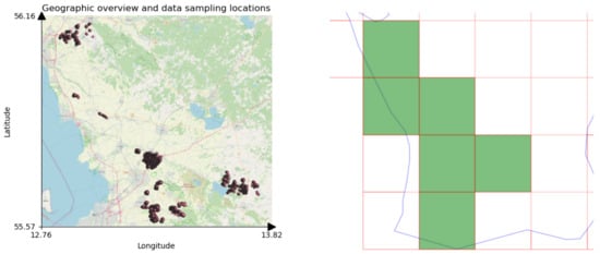
Figure 3.
A geographical overview of the data. The left figure shows the locations of the fields in southwest Sweden. The figure to the right shows the same region where the green tiles represent the regions/patches of Sentinel-1 data downloaded. These patches were selected in order to cover all the fields.
3.2. Sentinel-1 Data
The Sentinel-1 data were captured with acquisition mode IW swath, Level-1 product, GRD, resolution , with added orthorectification, and radiometric calibration over fields in Skåne (Figure 3) for a chosen time period over the years of interest. The years of interest were 2017, 2018, 2019, and 2020 and the chosen time period for the input data was April 1st until the end of July (Figure 4). We selected these years due to the free availability of satellite data.
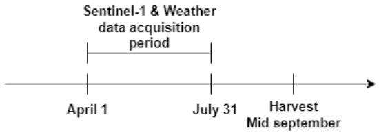
Figure 4.
The Sentinel-1 and weather data were collected from the first of April until the end of July. This end date is approximately a month before harvest, which for winter wheat typically occurs in mid-September in Sweden. In general, however, we only retained a single contribution per week from each of our three input data sources (Sentinel-1, weather, or topography). For Sentinel-1, this was performed by selecting the first RFI-free image from that week. For weather, the daily measurements were accumulated over the whole week.
During that time period, we were able to obtain 2–3 input data contributions from Sentinel-1 each week. We also note that this contribution was possible to obtain regardless of the type of weather. However, due to the occurrence of RFI, we decided to only choose a single sample each week—the first sample during that week, which produced VH and VV band values without RFI. It was possible to obtain such an RFI clean sample for the vast majority of the chosen time period. In general, we only retained a single contribution per week from each of our three input data sources (Sentinel-1, weather, or topography).
3.3. Filtering Speckle Noise
Sentinel satellites based on SAR technology have the ability to penetrate clouds and collect data at all hours of the day. SAR data, however, come with some drawbacks. One serious drawback is that SAR can be affected by speckle noise (Figure 5), which must be removed before the data can be interpreted by machine learning models. Speckle noise is a result of a physical limitation of SAR technology, and occurs when multiple radio waves are reflected back to the satellite from a single-resolution cell on the ground. This noise is modeled as a product of that underlying reflectivity. Many noise reduction methods, however, are based on the assumption of additive noise and cannot be applied to clean such speckle noise data.
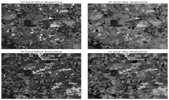
Figure 5.
Images for VV and VH polarizations before and after applying the transformation and despeckling. The process may have caused some loss of sharpness, but it is generally a significant improvement compared to more traditional speckle filtering techniques [9].
A new ML-based approach for despeckling SAR data called SAR2SAR was recently developed in [21]. This method is an extension of an earlier idea called Noise2Noise [22] and uses self-supervised learning with the ability to restore noisy data without ever seeing clean examples. This approach is an improvement over traditional methods, such as Gaussian, median, or Lee filters [9,21], which usually distort the images and cause information loss.
Despeckling with the SAR2SAR approach has its own challenges. For the method to work, we discovered that the data for both distributions, our raw Sentinel-1 data and the data which the original SAR2SAR model was trained upon, must match. If the data match, then transfer learning will be possible. We resolved this by developing a transform which, given a polarization p, aligns each pixel x in a given image X to match, distribution-wise, the original training data of the SAR2SAR model,
The main reason for the two different definitions of the transformation T in (1) is that the underlying distributions are different depending on whether the polarization p is VH or VV. The proposed transformation further ensures that the result can never be zero, which also helps to avoid issues when working with satellite indices. (We used , but all values for produce similarly good results).
3.4. Yield Data
The raw yield data are automatically gathered by combine harvesters and consists of discrete yield values in space and time. The raw data were collected from fields of different sizes, ranging from small fields of 1 hectare up to large fields of 180 hectares. This raw data, however, must be further aggregated and cleaned before it can be used for training the machine learning (ML) algorithms. We created a grid that summarizes the yield within grid blocks with areas of . All the data points within a 25 m radius of the center coordinate of each grid block were averaged in order to produce a single average yield value, in tons per hectare, for this grid block (Figure 6). These center grid coordinates will also be used as guidelines in terms of how to put together the training data as well. This allows consistency during data collection but, most importantly, avoids any possible issues with data leakage [23] during the training of the ML algorithms later. Data leakage occurs when information from one data point overlaps another data point. By choosing grids that are 50 m apart and have centers with a 25 m distance, as can be seen in the middle part of Figure 6, we guarantee that there will be no overlap or duplicated information in our data.
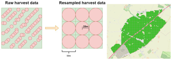
Figure 6.
Illustration of the unevenly distributed points in the raw yield data and how they were resampled into a grid.
As can be seen in Figure 7, the amount of yield data varied significantly over each of the years chosen in this study, as did the number of participating fields.
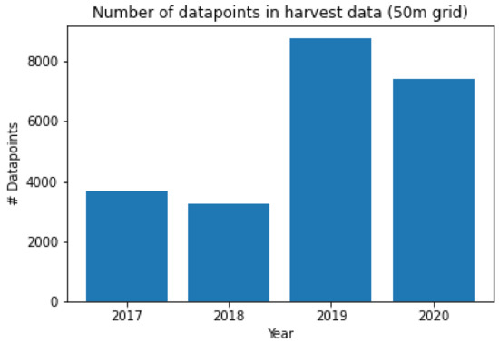
Figure 7.
Winter wheat yield data available for training for each of the study years under the chosen grid. The number of fields where the above data were obtained during the years 2017, 2018, 2019, and 2020 were 49, 31, 132, and 88, respectively.
3.5. Auxiliary Data
To further improve the predictions, we also enriched the Sentinel-1 training data with other auxiliary data (see Table 1). These data are grouped into three main categories: weather, elevation, and topographical classification. The weather data were obtained from a collection of joined Swedish public databases (The public databases used were Lantmet, Trafikverket, Fieldsense, and partly SMHI) containing historical weather data. Since the density of weather stations is much lower than the density of yield data, we only sampled from the closest weather station for each field. Since we used a weekly timescale, we decided to resample the daily weather data into accumulated weekly weather data in order to follow the time range of the other data in our collection (Figure 4). The elevation data were obtained from Skogsstyerlsen [24], which was collected with laser scanners attached to airplanes. The topographic classification was created by feeding the elevation data to the Grass GIS geomorphon algorithm [25]. All such auxiliary training data will be used in a successive fashion in order to understand the benefits, if any, to the model due to their incremental inclusion.

Table 1.
Description of auxiliary training data used.
3.6. Models
In this work, we employ two different machine learning approaches: the light gradient boosting machine (LGBM) and the Feed-forward Neural Network (FNN).
The LGBM is a machine learning model based on decision trees that belong to a family of Gradient Boosting Decision Tree (GBDT) models [26]. LGBM utilizes Gradient-based One-Side Sampling and Exclusive Feature bundling (EFB). As a result, the model learns to exclude a significant proportion of data with small gradients, which is a particularly useful aid when the feature importance is unknown. Furthermore, EFB bundles mutually exclusive features together to decrease the number of features and results in speeding up the training process with almost no loss in accuracy. The default hyperparameters [27] were used unless explicitly stated otherwise. Additionally, LGBM provides built-in support for extracting feature importance. We use this capability under the default LGBM "split" setting to uncover information about which of the input data features are most important towards the result, predicting yield.
The other machine learning method we employ is the FNN, which is the quintessential deep learning model mimicking a network of neurons in the brain (hence neural network) by a cyclic-directed graph of nodes [28]. When designing an FNN, the depth and width of the hidden layers, activation functions, and regularization need to be considered [28,29,30,31]. We decided to have a depth of 6 hidden layers with a width that varies depending on the number of features, , as follows:
- Hidden Layer 1 width ≔ ;
- Hidden Layer 2 width ≔ ;
- Hidden Layer 3 width ≔ ;
- Hidden Layer 4 width ≔ ;
- Hidden Layer 5 width ≔ .
For each hidden layer, we employ a Rectified Linear Unit (ReLU) activation function. The output layer was always a single node with linear activation, as this was a regression problem. We chose an Adams gradient descent optimizer with default hyperparameters [32], as tests have shown that this is a good optimizer when used with adaptive learning rates [30]. We implemented a mean squared error loss function. A maximum of 50 epochs were used, with an early stopping scheme monitoring the validation loss with 10 epochs of patience used to regularize and stop overfitting. The validation set was randomly picked to be of the training set, and the batch size was 32. No further tuning of the networks was considered.
The reason for considering the above two models is that we would like to compare how a classic yet simple FNN model would compare against a very powerful decision tree model such as the LGMB.
3.7. Metrics
To evaluate our machine learning models, we use classic metrics such as the root mean squared error (RMSE), accuracy (Acc.), and weighted F1-score (F1), whose details can be found in [33]. We provide the equations also in Appendix A for completeness. These metrics can be used for both regression and classification tasks [34]. Yield prediction is a regression problem but can be reformulated as a classification problem by rounding yield values [17]. This will also allow us to somewhat compare how Sentinel-1 performs against Sentinel-2 for yield prediction for winter wheat. For a detailed description of how the rounding was performed, please see Appendix B.
3.8. Resolutions and Sampling
Our dataset is created from a total of 49, 31, 132, and 88 fields for the years 2017, 2018, 2019, and 2020, respectively, (Figure 7). Some such fields were located next to each other, while some other fields were far apart, as can also be seen in Figure 4. We trained a different algorithm for each data year. Therefore, for each such year, we randomly split the corresponding data into training and testing sets at a ratio of 80:20.
When creating these datasets, we had to take the different resolutions (Figure 8) of the data into account. The yield data had a lower resolution (50 × 50 ) compared to Sentinel-1 (11 × 11 ), topography (10 × 10 ), and elevation data (10 × 10 ).
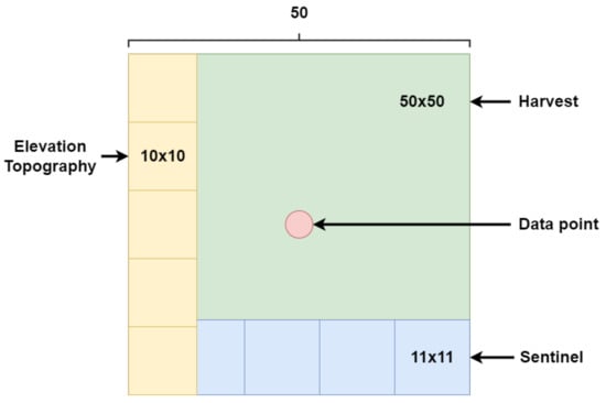
Figure 8.
Visualization of the mismatch in resolution between the yield, Sentinel-1, topography, and elevation data. The lowest resolution was given by the yield data, where each data point summarizes yield within a 50 × 50 area. The satellite data had a finer resolution of 11 × 11 , while the topography and elevation data shared a resolution of 10 × 10 . This resolution difference was the reason for introducing grid sampling instead of just sampling the nearest data point in space.
To better examine possible effects due to the mismatching resolutions, two different sampling approaches were adopted when creating the feature vectors: nearest and grid sampling. For given longitude and latitude coordinates, nearest sampling simply ignored the resolution mismatch and picked a single sample nearest in space for each of the different features: Sentinel-1, topography, and elevation. For grid sampling, a neighborhood of data points was picked to form a 3-by-3 grid. The data point closest in space was the center point. From the center point, all neighboring data points in directions north, northeast, east, southeast, south, southwest, west, and northwest (8 additional data points) were added. In the result section, we will use to signify the sampling method and resolution: where G = grid, N = nearest, and the number 50 signifies the grid resolution in meters.
3.9. Datasets and Feature Vectors
To better understand the benefits of the inclusion of different features, we created six smaller datasets which can be seen in Table 2. This allows us to evaluate the benefits of each dataset as we successively add them to our training data. This gives us an easy way to compare the relative importance of each data source. The purpose of the random feature vector seen in Table 2 was to have a baseline for comparison purposes.
Table 2.
List of different features used in this study and their sizes. Also, note that a random feature is included as a control to uncover a baseline for comparisons.
4. Results
One of the first questions which we consider in this work is whether a machine learning model can learn to predict yield from Sentinel-1 data. To address this question, we evaluated the RMSE for the G-50 grid as we incrementally increased the size of the VH-VV data. For this test, we chose to train the LGBM model with a 5-fold cross-validation scheme. The hyperparameters for the LGBM model were set at their default values [27] of 2000 boosted trees. Furthermore, an Early Stopping scheme with patience (stopping_rounds) of 200 boosting iterations was used to prevent overfitting. We present the RMSE on the test data (20% of the dataset) in Figure 9 as we incrementally increase the total size of the data. These results answer our question conclusively since the RMSE is gradually decreasing. There is information in the Sentinel-1 data that our algorithm is able to learn. We discuss this finding from a wider perspective again later in Section 5 below.
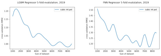
Figure 9.
The regression RMSE decreased as the size of the dataset increased, with grid G-50 and input VH-VV from Sentinel-1. This result indicates that the Sentinel-1 data contain valuable information for predicting 2019 yield. Results from LGBM (left) and FNN model (right).
Reconstructing and comparing the predicted yield distributions with the true yield distributions gives another insight into how well a model performs. Using the data from 2017 to 2020, the LGBM model with G-50, and the All feature vector, we obtain the distributions shown in Figure 10, Figure 11, Figure 12 and Figure 13. The predicted distributions are similar in shape, mean, and variance to the true distribution of the yield for that year. The predicted distributions shown in Figure 10, Figure 11, Figure 12 and Figure 13 are based solely on testing data, and the right figures are based on the training data. The height difference on the y-axis is due to the size difference between the training (80%) and test (20%) datasets. From the Figures, we can see that the yield distribution is non-stationary and varies significantly from year to year.
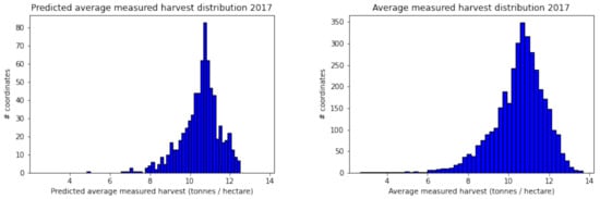
Figure 10.
The predicted yield distribution for 2017 (left), obtained using an LGBM model with grid G-50 and input “All features”, closely matched the true yield distribution (right). The model accurately captured the shape, mean, and variance of the true distribution for this year.
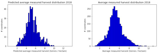
Figure 11.
The predicted yield distribution for 2018 (left), obtained using an LGBM model with grid G-50 and input “All features”, closely matched the true yield distribution (right). The model accurately captured the shape, mean, and variance of the true distribution for this year.
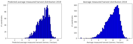
Figure 12.
The predicted yield distribution for 2019 (left), obtained using an LGBM model with grid G-50 and input “All features”, closely matched the true yield distribution (right). The model accurately captured the shape, mean, and variance of the true distribution for this year.
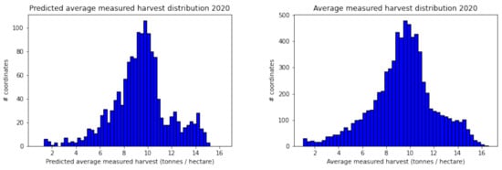
Figure 13.
The predicted yield distribution for 2020 (left), obtained using an LGBM model with grid G-50 and input “All features”, closely matched the true yield distribution (right). The model accurately captured the shape, mean, and variance of the true distribution for this year.
More detailed overall results, broken down by year, model, feature vector , and grid type , are shown in Table 3. We note that the best score of 0.75 RMSE was achieved using G-50 with the LGBM model for yield data from 2018. However, we see that the N-50 results of 0.76 were not far behind. In general, we observe that by using Grid sampling instead of Nearest sampling, we obtain a ∼1.3% increase in performance. There are, however, also configurations for which the sampling methods perform the same. Another general trend is that the VH-VV feature vector scores the best out of the feature vectors containing data from one single source. We note also that the VH-VV feature vector was also close in score to the All feature vector, having only an ∼8% decrease in performance. The other individual feature vectors scored, in general, worse. Specifically, the next best feature vector was weather, followed by elevation, and then, in last place, topography, which performed worst of all the individual feature vectors for our models. Furthermore, the results in Table 3 clearly show that the LGBM model outperforms the FNN model in all aspects. This is also mainly the reason for using the LGBM model for most of the other comparisons and results presented in this work.
Table 3.
RMSE for each year, model, feature vector, sampling method, and resolution. The LGBM model outperforms the FNN model in all cases. There seems to be a slight advantage to using Grid sampling. Note that weather is not presented with the Grid sampling method, since we only sample from one weather station per field.
To better understand and evaluate performance by the LGBM model, we also present the classification scores separately for each year in Table 4. See Appendix B for the methodology followed to convert regression values to classes. Based on the results in this table, we see, for instance, that ∼83% of the predictions are within a maximum error of 1 ton/hectare in 2017.
Table 4.
Classification accuracy and F-1 score based on varying error tolerance, in tons/hectare, based on the LGBM model trained with G-50 and All features. Note that the performance increases significantly between .
To put the findings from Table 3 and Table 4 into perspective, we also computed the equivalent results from the control, random feature, using the N-50 grid. We found an average RMSE of 1.89, an average accuracy of 45.5%, and an average F1 score of 37%. Comparing the results in Table 3, we observe that the average RMSE for the random data increased by a factor of ∼2.12 compared to the top average RMSE of 0.89 tons per hectare (over all years). Similarly, for the average accuracy and average F1-score, we saw a decrease of about 43.1% and 53.5%, respectively, when compared with the respective average accuracy and F1-score from that table.
In order to uncover the role that each of the input features played towards producing these results, we made use of the feature importance library [33], which is already built-in for LGBM models. We present these results in Table A2 in Appendix D. The full results, including plots, can be found in this project’s GitHub repository [35]. To summarize the results over all years, we see that the despeckled Sentinel-1 VH and VV band at around week 19 to 25 is always among the top five most important features. We also see height consistently showing up among the top 10 most important features. Weather and topographical classification is significantly less important and shows up around place 30, with an importance score almost a magnitude smaller than the Sentinel-1 and height data. We discuss these results further in the following section.
5. Discussion
One would expect that the performance of a machine learning model would improve with more data. This is because the data are assumed to have a pattern that the model can learn from. If this is not the case, it suggests that there is nothing in the data that algorithms can learn or that the data contain other errors, such as, for instance, RFI. We saw in Figure 9 a decrease in the RMSE for both models tested as we increased the dataset size, implying that the Sentinel-1 data we collected indeed contain valuable information for winter wheat yield prediction.
The LGBM model was shown to be sufficiently powerful for yield prediction and outperformed the FNN model in all aspects, achieving better performance and significantly faster training times. For example, running a 5-fold iteration with LGBM using the data from 2017 and the G50 feature vector took 2.4 s, while the same set-up with FNN took 37.7 s (∼16 slower). The LGBM model was further able to capture the varying yield distributions for each year studied, mimicking the shape, mean, and variance of the true yield. The model also includes built-in feature importance methods [26] for quickly finding the most important features contributing to the result, while the FNN model does not. We also tested simpler models, such as linear and logistic regression (results not presented here). These simpler models, however, failed to reach the performance of the LGBM model.
We have shown how grouping the raw yield data into bins which are laid out in a grid pattern gives a simple way to construct a dataset suitable for training a yield prediction model, and is useful for controlling potential data leakage. We obtained a barely significant RMSE decrease when using grid sampling compared to just using the center pixel at each yield data point. This shows that we do not add much information when we include the neighboring pixels, which could explain why we are not seeing a more significant RMSE decrease. The local spatial correlations of despeckled SAR data, therefore, must be high and not add much new information to the learning process. The first law of geography states, “Everything is related to everything else. However, near things are more related than distant things” [36]. One way to further understand such phenomena would be to consider spatial-cross-validated training methods.
We found that the Sentinel-1 data contain three fundamental problems which need to be addressed before any data processing and learning occurs. These problems relate to missing data, speckle noise, and radio frequency interference (RFI). We have presented solutions for two of these issues. We addressed the missing data by only using one sample per week. We also construct a transformation that allows us to apply the SAR2SAR method in order to then remove most of the speckle noise while still retaining a high sharpness in the image. We noticed that with our transformation and SAR2SAR despeckling, we obtained an accuracy increase of 10–15% depending on the dataset. We also tried to address the third issue, the RFI, by constructing a simple RFI filter consisting of morphological operations. However, this did not increase our performance, and we concluded, therefore, that a more sophisticated filtering algorithm would be needed to more effectively remove RFI. We, therefore, leave this task as future work.
Topographic classification may not be a useful feature, at least not in the way it was utilized in this project, where the classification was represented through one-hot encoding. Similarly, weather data were found to have a low feature importance score, which seems counter-intuitive since the weather is commonly known to be an important feature for crop development. A possible explanation for this low feature importance score, however, is that the Sentinel-1 data are correlated with the moisture content of crops, which also depends on weather conditions [11].
6. Conclusions
We have presented a general machine learning modeling approach to predicting winter wheat yield using primarily SAR data from Sentinel-1. More importantly, we have shown that Sentinel-1 Interferometric Wide Swath data contain valuable information for predicting winter wheat yield. In summary, we found that by implementing despeckling for the Sentinel-1 data and combining them with all other features, the LGBM model reached an average RMSE of 0.89 tons per hectare, an average accuracy of 80%, and an average F1-score of 79.5%.
We tried to further assist the models during their training by also including some of the typical SAR satellite indices such as RVI and Ratio [37]. However, these extra indices did not help to improve the model performance, and as a result, we do not include them here.
We propose three extensions of our work to reach the main goal of operational use of the models. The first extension relates to using a convolutional neural network-based model in order for spatial correlation to be naturally taken into account by the model. We have shown that these correlations are important and should be leveraged. To create images as input data to the model, one can use n-by-n samples from the coordinate-wise yield grid and their respective Sentinel-1 data. The second extension relates to combining Sentinel-1 SAR backscatter with Sentinel-2 optical imagery, since it is possible that the two different types of imagery can contain mutually exclusive information important for yield prediction. The final extension relates to testing the generality of our approach for other crops. For example, we noted that changes in the rapeseed fields next to the winter wheat fields in Skåne were reflected rather well in the Sentinel-1 SAR backscatter time series.
To aid further work, we provide in a GitHub repository [35] the python algorithm, which was used to produce the findings and results discussed in this article.
Author Contributions
Conceptualization, S.M., A.O. and A.S.; methodology, O.P.B., C.S., S.M., A.O. and A.S.; software, O.P.B., C.S. and A.S.; validation, O.P.B., C.S. and A.S.; formal analysis, O.P.B., C.S., S.M., A.O. and A.S.; investigation, O.P.B., C.S., S.M., A.O. and A.S.; resources, O.P.B., C.S., S.M., A.O. and A.S.; data curation, O.P.B., C.S., S.M., A.O. and A.S.; writing—original draft preparation, O.P.B., C.S. and A.S.; writing—review and editing, O.P.B., C.S., S.M., A.O. and A.S.; visualization, O.P.B., C.S. and A.S.; supervision, A.S.; project administration, A.S.; funding acquisition, S.M., A.O. and A.S. All authors have read and agreed to the published version of the manuscript.
Funding
The work in this study is partially supported by Vinnova grant number 2020-03375 and Rymdstyrelsen grant number 2022-00282.
Institutional Review Board Statement
Not applicable.
Data Availability Statement
Data available on request due to privacy restrictions. The data presented in this study are available on request from the corresponding author. The data are not publicly available due to possibility to identify locations of participating farms.
Acknowledgments
The work for A.S. is partially supported by grants from Vinnova 2020-03375, eSSENCE 138227, Rymdstyrelsen 2022-00282, and Formas. The training and data handling was enabled by resources provided by the Swedish National Infrastructure for Computing (SNIC), partially funded by the Swedish Research Council through grant agreement no. 2018-05973. Data from Copernicus, Sentinel-1, and Sentinel-2 satellites acquired were made possible through a grant from the European Space Agency under research project ID 1b2882.
Conflicts of Interest
The authors declare no conflict of interest. Some of the data in this study were provided by the T-Kartor AB and Niftitech AB databases. The funders had no role in the design of the study; in the collection, analyses, or interpretation of data; in the writing of the manuscript, or in the decision to publish the results.
Abbreviations
The following abbreviations are used in this manuscript:
| ML | Machine learning |
| Mg | Magnesium |
| pH | Potential of hydrogen |
| CO | Carbon dioxide |
| CaCO | Calcium carbonate |
| NIR | Near infrared |
| SWIR | Shortwave infrared |
| RGB | Red green blue |
| NDVI | Normalized difference vegetation index |
| NDWI | Normalized difference water index |
| LGBM | Light gradient boosting model |
| SHAP | Shapley values |
| RMSE | Residual mean square error |
Appendix A. Definition of Metrics
Let be the ground truth measurement from the yield data, be the predicted value, be True/False positive, and be True/False negative. Then, the metrics used are defined as follows:
Appendix B. Creating Classes from RMSE
An important problem to consider when rounding to the nearest integer to create classes is that close prediction in yield might produce different classes and vice versa. For example, say the true yield was 6.51 (rounded to 7) tons and that the predicted yield was 6.49 (rounded to 6). The prediction would then be very close and an excellent estimation, but still be counted as an incorrect classification. In contrast, an objectively worse prediction, say 7.49 (rounded to 7), would be counted as a correct classification, even though there is a significantly larger error. This issue is due to the task of yield prediction fundamentally being a regression task and not a classification task. Hence, just rounding to the nearest integer skews the results and should not be used.
A better way of rounding would be to take the RMSE into account. For instance, we want RMSE predictions that are within some error tolerance, , to be assigned the same class as the true yield. To do this, we start by creating our classes. We will use the non-negative integers as our classes, i.e., 0, 1, 2, etc., which is what the authors did in the study using Sentinel-2 [17]. Now, given that the true yield and predicted yield are within some error, we want both to belong to the same class. Let us illustrate this with an example. Given that the error tolerance is , the true yield is 10.7, and the predicted yield is 10.3, we see that the absolute value of the difference will be . Because the value is within the error tolerance, this will be a correct classification. How should we round to make this the case? If we blindly rounded to the nearest integer, we would have true yield class 11 and predicted yield class 10. We instead perform the following: If the prediction is within the tolerance, set the prediction to the same class as the true yield regardless of rounding, i.e., 10.3 is set to 11 in our example. Note that, for the true yield, we always perform integer rounding. It is just the predicted yield that needs extra attention. Another example, given that the error tolerance is , the true yield is 10.7, and the predicted is 11.4, we see that the absolute value of the difference will be . The value is not within the error tolerance, and as such, the rounding needs to be performed so they do not share the same class. Here, we see another issue that needs special attention. If we just rounded both numbers independently, then we would obtain 11 as the true yield class and predicted yield class. Therefore, we added extra conditions in our code to handle this. The code checked first if the prediction was within the error tolerance, and if it was not, then we rounded both independently to classes. If the prediction was not within the error tolerance and the true and predicted yield were rounded to the same class, then the predicted yield was changed to a class above or below the true yield. In the previous example, because the predicted yield was , the class was changed from 11 to 12. If the predicted yield was lower, then the class would instead have been 10. Note that this alters the notion of a clearly defined class, but is what we found to be the best way to handle the issues by just rounding to the nearest integer. Unless otherwise stated, we will use the same default value of as authors in [17] for our classification results.
Appendix C. Results Using Linear Regression
In the table below, we show the results using a simple Linear Regression (LR) model on our data for all years, Table A1. The value of in the table is 4948928042 due to the LR model not converging.
Table A1.
Comparisons of RMSE results based on simple Linear Regression and data from all years.
Table A1.
Comparisons of RMSE results based on simple Linear Regression and data from all years.
| 2017 | 2018 | 2019 | 2020 | ||
|---|---|---|---|---|---|
| LR | LR | LR | LR | ||
| G-50 | All | 0.99 | 0.85 | 1.08 | 1.31 |
| VH-VV | 1.12 | 0.91 | 1.23 | 1.74 | |
| Topography | 1.35 | 1.50 | 1.80 | 2.65 | |
| Elevation | 1.30 | 1.33 | 1.75 | 2.64 | |
| N-50 | All | 0.93 | 0.83 | 1.08 | 1.28 |
| VH-VV | 1.08 | 0.89 | 1.26 | 1.72 | |
| Weather | 1.13 | 1.34 | 1.66 | ||
| Topography | 1.32 | 1.48 | 1.80 | 2.64 | |
| Elevation | 1.30 | 1.38 | 1.81 | 2.65 |
Appendix D. Feature Importance Scores
In Table A2 below, we show the feature importance scores given by the model. A higher number indicates that the feature is more important. The features listed are topographical height denoted as “height” as well as the signal type (vv or vh) and finally, from which week each signal was obtained. As an example, therefore, vv-week-23 denotes the vv Sentinel-1 signal data received from week 23. It is interesting to note that either vv or vh Sentinel-1 data from week 20 and up to week 24 seemed to be very important in producing the resulting yield predictions regardless of year. Please refer to the project’s GitHub repository for complete results and related plots [35].
Table A2.
Comparisons of feature importance scores over different years.
Table A2.
Comparisons of feature importance scores over different years.
| 2017 | 2018 | 2019 | 2020 | ||||
|---|---|---|---|---|---|---|---|
| Feature | Score | Feature | Score | Feature | Score | Feature | Score |
| vv-week-23 | 1633 | vh-week-21 | 1299 | vh-week-21 | 1866 | vv-week-24 | 1747 |
| vh-week-24 | 1169 | vv-week-22 | 1291 | vh-week-19 | 1457 | vh-week-15 | 1596 |
| vv-week-19 | 1054 | vv-week-27 | 1201 | vv-week-17 | 1444 | vh-week-16 | 1592 |
| vh-week-15 | 1039 | vh-week-25 | 1191 | vh-week-14 | 1416 | height | 1591 |
| vh-week-14 | 1028 | vv-week-26 | 1155 | vv-week-24 | 1408 | vv-week-26 | 1562 |
| vv-week-29 | 1019 | vh-week-22 | 1090 | vv-week-14 | 1273 | vh-week-20 | 1500 |
| height | 980 | vv-week-21 | 1026 | vv-week-22 | 1227 | vh-week-28 | 1493 |
| vv-week-22 | 974 | height | 1006 | vh-week-26 | 1213 | vh-week-14 | 1483 |
| vv-week-14 | 948 | vh-week-28 | 1006 | vh-week-20 | 1198 | vv-week-14 | 1437 |
| vv-week-24 | 934 | vv-week-29 | 1002 | vv-week-16 | 1163 | vv-week-27 | 1430 |
References
- Springer. Precision Ag Definition. 2019. Available online: https://www.springer.com/journal/11119/updates/17240272 (accessed on 2 September 2022).
- Liaghat, S.; Balasundram, S. A Review: The Role of Remote Sensing in Precision Agriculture. Am. J. Agric. Biol. Sci. 2010, 5, 50–55. [Google Scholar] [CrossRef]
- Maki, M.; Sekiguchi, K.; Homma, K.; Hirooka, Y.; Oki, K. Estimation of rice yield by SIMRIW-RS, a model that integrates remote sensing data into a crop growth model. J. Agric. Meteorol. 2017, 73, 2–8. [Google Scholar] [CrossRef]
- Kasampalis, D.A.; Alexandridis, T.K.; Deva, C.; Challinor, A.; Moshou, D.; Zalidis, G. Contribution of Remote Sensing on Crop Models: A Review. J. Imaging 2018, 4, 52. [Google Scholar] [CrossRef]
- Bhatia, A. Modelling and Simulation of Diffusive Processes; Basu, S.K., Kumar, N., Eds.; Methods and Applications; Springer International Publishing AG: Cham, Switzerland, 2014. [Google Scholar]
- Betbeder, J.; Fieuzal, R.; Baup, F. Assimilation of LAI and dry biomass data from optical and SAR images into an agro-meteorological model to estimate soybean yield. IEEE J. Sel. Top. Appl. Earth Obs. Remote. Sens. 2016, 9, 2540–2553. [Google Scholar] [CrossRef]
- Veloso, A.; Mermoz, S.; Bouvet, A.; Le Toan, T.; Planells, M.; Dejoux, J.F.; Ceschia, E. Understanding the temporal behavior of crops using Sentinel-1 and Sentinel-2-like data for agricultural applications. Remote. Sens. Environ. 2017, 199, 415–426. [Google Scholar] [CrossRef]
- Vreugdenhil, M.; Wagner, W.; Bauer-Marschallinger, B.; Pfeil, I.; Teubner, I.; Rüdiger, C.; Strauss, P. Sensitivity of Sentinel-1 Backscatter to Vegetation Dynamics: An Austrian Case Study. Remote. Sens. 2018, 10, 1396. [Google Scholar] [CrossRef]
- Sentinel Hub. Sentinel-1 GRD. Available online: https://docs.sentinel-hub.com/api/latest/data/sentinel-1-grd/ (accessed on 11 October 2022).
- The European Space Agency. Sentinel-1. Available online: https://sentinel.esa.int/web/sentinel/missions/sentinel-1 (accessed on 11 October 2022).
- Khabbazan, S.; Vermunt, P.; Steele-Dunne, S.; Ratering Arntz, L.; Marinetti, C.; van der Valk, D.; Iannini, L.; Molijn, R.; Westerdijk, K.; van der Sande, C. Crop Monitoring Using Sentinel-1 Data: A Case Study from The Netherlands. Remote. Sens. 2019, 11, 1887. [Google Scholar] [CrossRef]
- Nasrallah, A.; Baghdadi, N.; El Hajj, M.; Darwish, T.; Belhouchette, H.; Faour, G.; Darwich, S.; Mhawej, M. Sentinel-1 data for winter wheat phenology monitoring and mapping. Remote. Sens. 2019, 11, 2228. [Google Scholar] [CrossRef]
- Weiß, T.; Ramsauer, T.; Jagdhuber, T.; Löw, A.; Marzahn, P. Sentinel-1 Backscatter Analysis and Radiative Transfer Modeling of Dense Winter Wheat Time Series. Remote. Sens. 2021, 13, 2320. [Google Scholar] [CrossRef]
- Palmisano, D.; Mattia, F.; Balenzano, A.; Satalino, G.; Pierdicca, N.; Guarnieri, A.V.M. Sentinel-1 Sensitivity to Soil Moisture at High Incidence Angle and the Impact on Retrieval Over Seasonal Crops. IEEE Trans. Geosci. Remote. Sens. 2021, 59, 7308–7321. [Google Scholar] [CrossRef]
- Harfenmeister, K.; Spengler, D.; Weltzien, C. Analyzing Temporal and Spatial Characteristics of Crop Parameters Using Sentinel-1 Backscatter Data. Remote. Sens. 2019, 11, 1569. [Google Scholar] [CrossRef]
- Harfenmeister, K.; Itzerott, S.; Weltzien, C.; Spengler, D. Detecting Phenological Development of Winter Wheat and Winter Barley Using Time Series of Sentinel-1 and Sentinel-2. Remote. Sens. 2021, 13, 5036. [Google Scholar] [CrossRef]
- Broms, C.; Nilsson, M.; Oxenstierna, A.; Sopasakis, A.; Åström, K. Combined analysis of satellite and ground data for winter wheat yield forecasting. Smart Agric. Technol. 2023, 3, 100107. [Google Scholar] [CrossRef]
- Skolnik, M.I. Radar Handbook; McGraw-Hill Professional: Toronto, ON, Canada, 1990; pp. 1.14–1.17. [Google Scholar]
- Leng, X.; Ji, K.; Kuang, G. Radio Frequency Interference Detection and Localization in Sentinel-1 Images. IEEE Trans. Geosci. Remote. Sens. 2021, 59, 9270–9281. [Google Scholar] [CrossRef]
- South Dakota State University. Radiometric Calibration. Available online: https://www.sdstate.edu/image-processing-lab/radiometric-calibration (accessed on 12 October 2022).
- Dalsasso, E.; Denis, L.; Tupin, F. SAR2SAR: A Semi-Supervised Despeckling Algorithm for SAR Images. IEEE J. Sel. Top. Appl. Earth Obs. Remote. Sens. 2021, 14, 4321–4329. [Google Scholar] [CrossRef]
- Lehtinen, J.; Munkberg, J.; Hasselgren, J.; Laine, S.; Karras, T.; Aittala, M.; Aila, T. Noise2Noise: Learning Image Restoration without Clean Data. arXiv 2018, arXiv:1803.04189. [Google Scholar]
- Kaufman, S.; Rosset, S.; Perlich, C. Leakage in Data Mining: Formulation, Detection, and Avoidance. In Proceedings of the 608 Proceedings of the 17th ACM SIGKDD International Conference on Knowledge Discovery and Data Mining, New York, NY, USA, 21–24 August 2011; KDD ’11. pp. 556–563. [Google Scholar] [CrossRef]
- Skogsstyrelsen. Skogliga Grunddata. 2022. Available online: https://www.skogsstyrelsen.se/sjalvservice/karttjanster/skogliga-grunddata/ (accessed on 1 September 2022).
- Jasiewicz, J.; Stepinski, T. Geomorphon. 2022. Available online: https://grass.osgeo.org/grass82/manuals/r.geomorphon.html (accessed on 1 September 2022).
- Ke, G.; Meng, Q.; Finley, T.; Wang, T.; Chen, W.; Ma, W.; Ye, Q.; Liu, T.Y. LightGBM: A Highly Efficient Gradient Boosting Decision Tree. Adv. Neural Inf. Process. Syst. 2017, 30, 3149–3157. [Google Scholar]
- Microsoft Corporation. LightGBM Regressor, Python API. Available online: https://lightgbm.readthedocs.io/en/latest/pythonapi/lightgbm.LGBMRegressor.html (accessed on 10 November 2022).
- Goodfellow, I.J.; Bengio, Y.; Courville, A. Deep Learning; MIT Press: Cambridge, MA, USA, 2016; Available online: http://www.deeplearningbook.org (accessed on 10 December 2022).
- Simonyan, K.; Zisserman, A. Very deep convolutional networks for large-scale image recognition. arXiv 2014, arXiv:1409.1556. [Google Scholar]
- Ruder, S. An overview of gradient descent optimization algorithms. arXiv 2016, arXiv:1609.04747. [Google Scholar]
- Zhang, C.; Bengio, S.; Hardt, M.; Recht, B.; Vinyals, O. Understanding deep learning requires rethinking generalization (2016). arXiv 2017, arXiv:1611.03530. [Google Scholar]
- Keras. Adam Optimizer Documentation. Available online: https://keras.io/api/optimizers/adam/ (accessed on 9 November 2022).
- SciKit-Learn. Metrics and Scoring: Quantifying the Quality of Predictions. Available online: https://scikit-learn.org/stable/modules/model_evaluation.html# (accessed on 8 November 2022).
- Naser, M.; Alavi, A. Insights into performance fitness and error metrics for machine learning. arXiv 2020, arXiv:2006.00887. [Google Scholar]
- Svenningsson, C.; Bogdanovski, O.P. Github sentinel 1 harvest prediction. Available online: https://github.com/Christoffer-Svenningsson/sentinel_1_harvest_prediction (accessed on 21 December 2022).
- Tobler, W.R. A Computer Movie Simulating Urban Growth in the Detroit Region. Econ. Geogr. 1970, 46, 234–240. [Google Scholar] [CrossRef]
- Holtgrave, A.K.; Röder, N.; Ackermann, A.; Erasmi, S.; Kleinschmit, B. Comparing Sentinel-1 and -2 Data and Indices for Agricultural Land Use Monitoring. Remote. Sens. 2020, 12, 2919. [Google Scholar] [CrossRef]


Disclaimer/Publisher’s Note: The statements, opinions and data contained in all publications are solely those of the individual author(s) and contributor(s) and not of MDPI and/or the editor(s). MDPI and/or the editor(s) disclaim responsibility for any injury to people or property resulting from any ideas, methods, instructions or products referred to in the content. |
© 2023 by the authors. Licensee MDPI, Basel, Switzerland. This article is an open access article distributed under the terms and conditions of the Creative Commons Attribution (CC BY) license (https://creativecommons.org/licenses/by/4.0/).