Beyond Trade-Off: An Optimized Binocular Stereo Vision Based Depth Estimation Algorithm for Designing Harvesting Robot in Orchards

Abstract

Depth estimation is one of the bottleneck parts for harvesting robots to determine whether the operation of grasping or picking succeeds or not directly. This paper proposed a novel disparity completion method combined with bilateral filtering and pyramid fusion to improve the issues of incorrect outputs due to the missed or wrong matching when achieving 3D position from 2D images in open-world environments. Briefly, our proposed method has two significant advantages in general. Firstly, occlusion between leaves, branches, and fruits is a universal phenomenon in unstructured orchard environments, which results in the most depth estimation algorithms facing great challenges to obtain accurate outputs in these occluded regions. To alleviate these issues, unlike other research efforts that already exist, we optimized the semi-global matching algorithm to obtain high accuracy sparse values as an initial disparity map; then, an improved bilateral filtering algorithm is proposed to eliminate holes and discontinuous regions caused by occlusion to obtain precise and density disparity outputs. Secondly, due to taking the practical high-efficiency requirements of the automated harvesting robot in its working status into consideration, we attempted to merge multiple low-resolution bilateral filtering results through the pyramid fusion model which goes beyond the trade-off mechanism to improve the performance of both accuracy and time cost. Finally, a prototype harvesting robot was designed to conduct experiments at three kinds of different distances (0.6~0.75 m, 1~1.2 m, and 1.6~1.9 m). Experiment results showed that our proposed method achieved density disparity maps and eliminated holes and discontinuous defects in the disparity map effectively. The average absolute error of our proposed method is 3.2 mm, and the average relative error is 1.79%. In addition, the time cost is greatly reduced more than 90%. Comprehensive experimental results demonstrate that our proposed algorithm provides a potential possibility for designing harvesting.

1. Introduction

Acquiring accurate distance between fruits and robots is the premise step to realizing automatic fruit grasping [1,2]. It is possible to exploit a RGB camera to achieve passive ranging, which has advantages of high resolution and strong anti-light influence ability [3]. Due to this, it is quite suitable for automated operations in an open-world environment [4]. The depth estimation methods based on the continuous images captured by the monocular camera have the advantages of simple structure and easy camera calibration; they also avoid the small field of view and difficult matching issues of stereo matching [5,6,7,8]. However, when the relative displacement between frames is large, it is easy to lose image frames and it is hard to match each other accurately. In addition, algorithms for monocular depth estimation always require massive calculations, which is not suitable for the spatial position calculation for fruit picking robots, which always require frequent movements during work. Obtaining depth map with multiple cameras makes it much easier to achieve accurate outputs; however, the transformation relationship between each camera’s coordinate systems is more complex. In addition, the time cost for matching multiple captured images is usually with a high time cost; this can hardly be applied for harvesting robots in practical applications [9,10,11,12,13]. Therefore, in order to drop the price cost, equipment volume, and weights of the automatic robot, reducing computational time cost and improving the accuracy of depth estimation is paramount. Binocular stereo cameras could be applied as a good choice for robots to acquire surrounding information. Therefore, we applied a baseline variable stereo camera (LenaCV USB 3.0), and the baseline was set as 60 mm.

Although binocular stereo vision has many great advantages, there are many challenges that have to be faced when designing an applicable depth estimation algorithm for harvesting robots in orchard environments [4,14,15]. The methods or algorithms based on binocular stereo vision still have issues with high matching time costs and incorrect matching outputs, etc., which restrict the further development of picking robots [16]. For example, in unstructured orchard environments, the phenomenon of occlusion between leaves, branches, and fruits commonly exists. When matching pixels or patches from a reference image to the target image, the discontinuous holes will easily appear due to the pixels in the reference image. It is then hard to find the corresponding pixels in the target image. Such wired values may lead to a disaster command when trying to grasp or move for the harvesting robot. Many CNN-based networks are trying to achieve depth estimation in auto-driving, which may alleviate this problem [17]. Massive data for training networks to obtain empirical outputs are unsuitable for our task yet. Thus, collecting images and calculating depth information in real-time can be regarded as an effective method. However, how to effectively process data to obtain a depth map is another inevitable challenge. To improve this issue, most efforts tried to reduce certain precision rates of disparity values to reduce total time cost. In contrast to these works, we tried to propose a method beyond the trade-off mechanism between accuracy and time cost, based on the consideration that the performance of accuracy rate and time cost are equally important for depth estimation algorithms.

In this paper, we study the principle of camera imaging, the transformation between different coordinate systems, etc. Based on these principles of binocular positioning, we present a novel completion method combined with bilateral filtering and pyramid fusion for disparity (Completion-BiPy-Disp) to improve the issues of incorrect outputs due to the missed or wrong matching when achieving 3D position from 2D images in open-world environments. Our proposed algorithm mainly has the following three contributions:

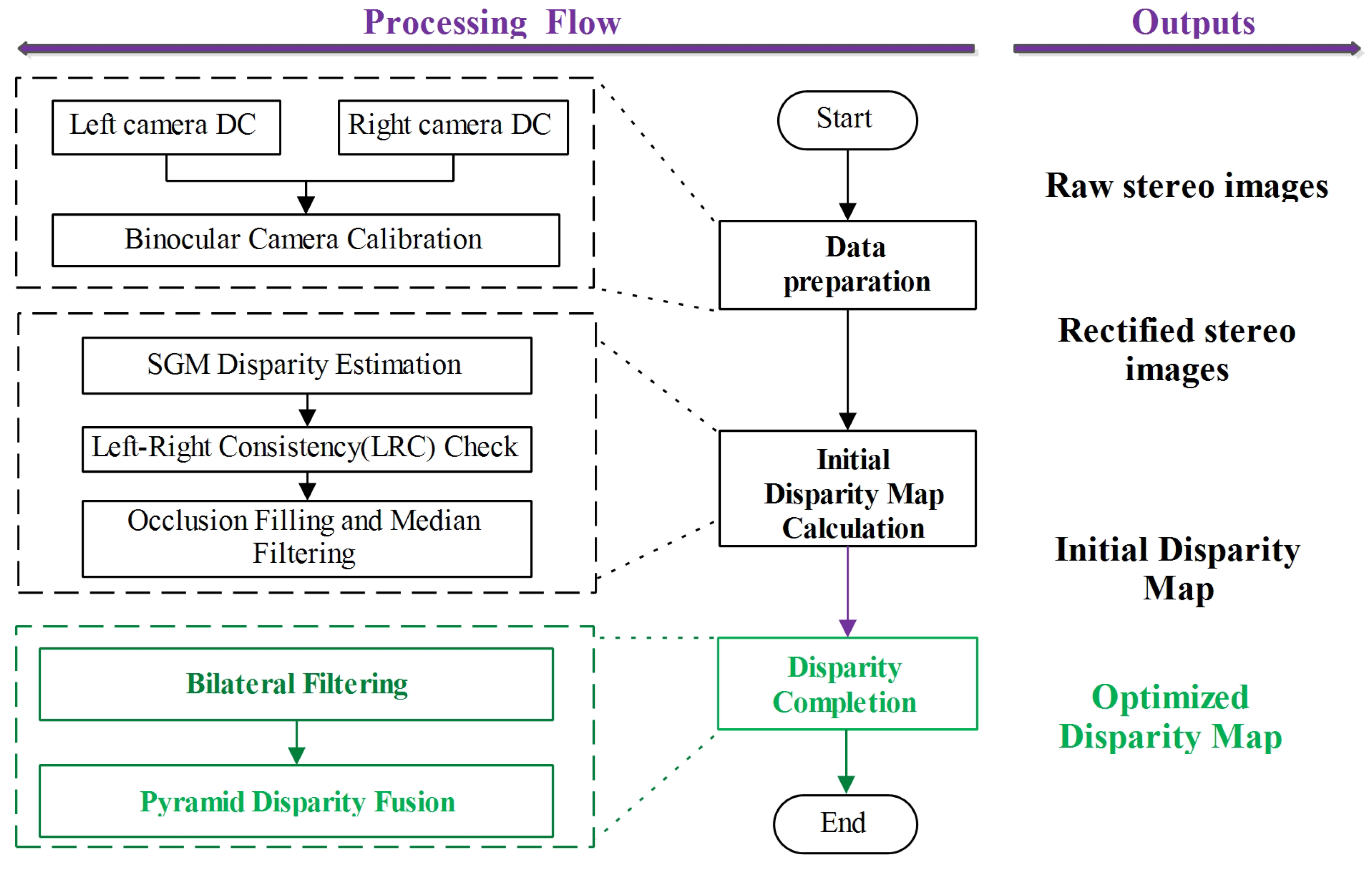
• We propose a completion method by applying a bilateral filtering (BF) algorithm on an optimized disparity map. Then, the high-precision sparse-optimized disparity maps are achieved by the semi-global matching algorithm with left and right consistency (LRC) checks and median filtering. In this way, discontinuous holes caused by missing or incorrectly matched corresponding pixels or regions from a reference image to the target image can be effectively attenuated.
• In order to reduce the time cost while maintaining the accuracy of outputs as much as possible, we attempted to merge multiple low-resolution bilateral filtering outputs into a pyramid model. This mechanism can optimize the accuracy of outputs while reducing the time cost effectively.
• A prototype harvesting robot was designed based on our proposed method. In addition, comprehensive qualitative and quantitative experimental results show that the proposed method has a certain validity in practical application.

2. Related Work

Acquisition of an accurate depth map is essential to realize automated harvesting operations. Basically, it can be divided into active and passive ranging according to the ways that measurements obtain information. Passive depth estimation could reconstruct 3D information from 2D images in a natural lighting environment. The approach can be divided into three categories based on the number of camera sensors used: monocular, binocular stereo, and multi-camera.

Monocular depth estimation uses only a RGB camera for image acquisition. For the issues of scale ambiguity when estimating depth from a single image, it is necessary to collect multiple consecutive images and perform stereo matching on different images through SfM (structure of motion) to calculate depth information, e.g., Roy and Isler [5] first proposed a motion estimation method to realize the registration and reconstruction of apple orchards, extract the number and diameter information of apples collected by a monocular camera, and realize the estimation of apple yield. Liu et al. [6] obtained continuous image data through a monocular camera and used the FCN model to segment fruits from background regions; they calculated the 3D position and size of the fruit by combining the results of segmentation with a motion estimation algorithm. Similarly, Häni et al. [7] used motion estimation on consecutive images obtained by a monocular camera to calculate the depth information of the fruit. Roy et al. [8] proposed a global feature-constrained solution proposed for predicting depth values for 3D reconstruction of orchard tree rows. Binocular stereoscopic vision is usually composed of a left and a right camera. Then, taking two images captured by these two cameras placed at different viewpoints, based on the principle of triangulation, the disparity image can be transformed into the depth image. Usually, by calculating the disparity between the left and right images, the final depth result can be obtained. In recent years, more and more research works have adopted binocular stereo vision-based methods to realize 3D position estimation for fruits [15,18]. Furthermore, binocular cameras were used as image acquisition equipment for many agricultural robots, such as strawberries [19,20], tomatoes [21,22], cucumbers [23], and oranges [24]. Such fruit harvesting robots always take stereo matching algorithms based on epipolar geometry to calculate the depth value between the robot and target fruit [4]. The theory of depth calculation using a multi-camera is similar to the binocular camera, which captures images from different cameras. These cameras are generally used to calculate the 3D position of detected objects [9,10,11,12,13].

To summarize, the use of passive sensors for depth computing has the advantages of strong environmental adaptability, flexible implementation methods, and low-price cost. Thus, it is being used in more and more practical fields [25,26,27]. Specifically, depth estimation based on monocular continuous images has the advantages of simple structure and easy camera calibration. However, when the relative displacement between frames is large, it is easy to lose some frames, leading to incorrect estimation results, and the depth estimation algorithm based on monocular always requires high computational cost which is not suitable for the practical 3D position estimation for fruit harvesting robots. Although depth information obtained by the multi-camera system could achieve high accurate outputs, the complex transformation of coordinate systems between cameras and the high time cost for matching images captured by multiple cameras make it unsuitable for picking robots that work in motion. However, the depth estimation by using binocular cameras has a good balance between the computational and time cost, so it is prevalently being applied by more and more picking robots.

3. Completion-BiPy-Disp Algorithm

Due to the critiques of obtaining a densely disparity map for an automatic harvesting or managing robot, high precious location estimation outputs and low time cost are always required at the same time in practical applications. Due to this motivation, we proposed a novel disparity estimation algorithm, Completion-BiPy-Disp, consisting of steps of data preparation, optimizing initial disparity map, and disparity map completion, as shown in Figure 1.

3.1. Data Preparation

In the beginning, we exploited the RGB camera to calculate the spatial positions of objects passively. It involves a sequential transformation, such as from space coordinates to camera coordinates, then to image coordinates and finally to pixel coordinates. Due to scale ambiguity issue caused by a single RGB image, a binocular camera was used to calculate the disparity map through the principle of triangle positioning. However, due to the limitations of binocular camera production or the producing craft, it is hard to guarantee that projecting a 3D point spatially to the left and right camera can also be at a same horizontal line. In order to match the image captured by the left and right cameras horizontally, we need to calculate the parameters of the stereo camera at first.

To obtain intrinsic and extrinsic parameters by using camera calibration method [28], we mapped a black-and-white checkerboard plane to the imaging plane of the camera, achieved the calibration of the camera according to the homograph correspondence between the planes, and obtained calibration parameters. In addition, this is because it is easy to obtain deviations by using only three angle calibration images. We use the maximum likelihood estimation method to improve distortion coefficients and perform parameter optimization. Finally, based on these parameters, we rectify each pair of stereo images which were captured by this binocular stereo camera and use rectified image pairs for disparity map calculation and optimization.

3.2. Optimize Initial Disparity Map

3.2.1. Initial Disparity Map

The basic principle of the SGM algorithm [29] is based on the idea of pixelwise matching of mutual information and approximating a global, 2D smoothness constraint by combining many 1D constraints. This SGM method calculates the matching cost hierarchically by mutual information. To pathwise optimize from all directions through the image, it uses an approximation of a global energy function named cost aggregation. Then, disparity computation is performed by winner takes all and is supported by disparity refinements such as consistency checking and sub-pixel interpolation. Thus, given one pair of binocular stereo images, $I_1$ and $I_2$, the entropy can be presented as $H_{I_1}$ and $H_{I_2}$, respectively. In a discrete space, we used Taylor expansion and summed the intensity as the joined entropy for a point p in the images, as in Equation (1):

$$H_{I_1,I_2}=\sum _{p=1}^P{h}_{I_1,I_2}(I_{1p},I_{2p})$$

(1)

specifically, $h_{I_1,I_2}(I_{1p},I_{2p})=-\frac{1}{n}log(p_{I_1,I_2}⨂g)⨂g$. p represents the distribution of intensity, g is the Gaussian convolution, n represents the number of corresponding points. The mutual information is defined as Equation (2):

$$M{I}_{I_1,I_2}=\sum _{p=1}^{P}m{i}_{I_1,I_2}(I_{1p},I_{2p})$$

(2)

where $m{i}_{I_1,I_2}(I_{1p},I_{2p})=h_{I_1}\left(i\right)+h_{I_2}\left(i\right)-h_{I_1,I_2}\left(i\right)$; the cost value $C_{MI}(p,d)$ can be defined as Equation (3):

$$C_{MI}(p,d)=-m{i}_{I_1,I_2}(I_{bp},I_{mq})$$

(3)

where $p(p_x,p_y)$ is a point in basic image $I_b$, and $q(q_x,q_y)$ is the corresponding point on the matching image $I_m$. d is expressed as the disparity value between point p and q. The coordinates of point q can be defined as Equation (4):

$$q={(p_x-d,p_y)}^T$$

(4)

Generally, computing the joint intensity distribution requires using an initial disparity map, initializing the disparity map, and randomly changing and optimizing the disparity map through an iterative strategy, which may result in inefficiency problems. By integrating multiple different angle cost matching, the SGM improves this deficiency effectively. The aim of the cost function is to minimize the cost path by accumulating all one-dimensional spaces with pixel p as the end point and disparity as d. The recursive calculation of the disparity d of the pixel p along a special path direction r calculates that its matching cost is $L_r(p,d)$, as Equation (5):

$$L_r(p,d)=c(p,d)+min\left(\begin{array}{c}{L}_r(p-r,d)\\ L_r(p-r,d-l)+P_1\\ L_r(p-r,d+l)+P_1\\ min{L}_r(p-r,i)+P_2\end{array}\right)-\underset{k}{min}\left(L_r(p-r,d)\right)$$

(5)

where the matching term $c(p,d)$ is the pixel-wise dissimilarity cost at pixel p with disparity d. Where $P_1$ and $P_2$ are two constant parameters, with $P_1<P_2$. To further preserve discontinuities, the gradient of the intensity can be set as Equation (6):

$$P_2=max(P_1,\frac{\widehat{P_2}}{I\left(p\right)-I\left(q\right)})$$

(6)

for each pair of pixels p and q. The accumulated cost is defined as Equation (7)

$$S(p,d)=\sum _r{L}_r(p,d)$$

(7)

Therefore, the initial disparity map is the value at each pixel is $\underset{d}{min}S(p,d)$.

3.2.2. Optimize

Although we obtained the initial disparity map from the excellent trade-off mechanism of accuracy and time cost performance of SGM algorithm, holes, incorrect points, or discontinuous regions still existed. Therefore, we applied two tricks for the initial disparity map. First, we applied a LRC check to avoid some outlier points generated by incorrect matching. That is, by traversing a point q of the epipolar line on a matching image, the disparity map $D_m\left(q\right)$ corresponds to the matching image. Then, we swapped the matching image and the base image to obtain the corresponding point of q, which we marked as p. Based on similar principles, we obtained the disparity map of $D_b\left(p\right)$. The continuity of $D_b$ and $D_m$ was verified with Equation (8) to determine the location of the occlusion or mismatched regions.

$$LRC\left(p\right)=-∥D_b\left(p\right)-D_m\left(q\right)∥$$

(8)

The lower the value of $LRC\left(p\right)$, the more stable the disparity value at this point. Otherwise, it means that the disparity value of p needs to be filtered or further optimized. Based on such constraints, incorrect matching points can be effectively reduced. The second trick is to remove small objects by minimum connected component detection and a median filter. Finally, we achieved a reliable optimized initial disparity map for the completion operation presented in the following steps.

3.3. Disparity Map Completion

3.3.1. Bilateral Filtering

The efficiency of the SGM algorithm largely depends on the displacement range set of the disparity and the resolution of the images to be matched. Although the efficiency of the SGM algorithm has been greatly improved compared with the global matching algorithm, the time cost of the algorithm is high when processing large resolution images. In addition, it is difficult to meet the requirements of practical applications due to outputs containing incorrect points or regions by the SGM algorithm. Therefore, we applied bilateral filtering up sampling (US) algorithm to join the RGB color image and its corresponding disparity map obtained based on the optimized SGM algorithm to preserve the boundary features of the image [30]. This method needs to provide a guide map I and a depth disparity map p in advance, and the output is the filtered disparity depth map q. The output $q_i$ is the filtered output at pixel i, which is the weighted average of the disparity map and color map at point i, defined as Equation (9):

$$q_i=\sum _j{W}_{ij}\left(I\right)p_j$$

(9)

where i and j are the indices of pixels, respectively, and the filter kernel $W_{ij}$ is a composed function of the guide image I and the independent image p. This is a linear filter of p. The bilateral filter kernel $W^{bf}$ is defined as Equation (10):

$$W_{ij}^{bf}=\frac{1}{K_i}{e}^{\frac{{∥X_i-X_j∥}^2}{{\sigma }_s^2}}{e}^{\frac{{∥I_i-I_j∥}^2}{{\sigma }_r^2}}$$

(10)

where X is the pixel coordinate, ${\sigma }_r$ and ${\sigma }_s$ adjust the intensity and spatial similarity, respectively, and according to recommendations, the values of ${\sigma }_s$ and ${\sigma }_r$ are set to 10 and 30, respectively. The normalization parameter $K_i$ is ${\displaystyle \sum _j}{W}_{ij}\left(I\right)p_j=1$. We use the original RGB low-resolution as the guiding image to filter the corresponding low-resolution disparity map, which obtains a disparity map in which the boundary region is well preserved.

3.3.2. Acquisition Multiscale Disparity Map

On the one side, the applied bilateral filter for full resolution requires a high time cost, and linear cubic interpolation may cause problems such as blurred boundaries, which would lose some key values. On another side, the result depended on a single disparity map. It is easy to face problems such as incorrect points or regions. Generally, disparity estimation algorithms are prone to take trade-off mechanisms between positioning accuracy and time cost. In fact, high precious location estimation outputs and low time cost are required always at the same time, in practical applications. Based on the above-mentioned problems and considerations, our method considers generating multiscale low-resolution disparity maps and fusing these disparity maps. The pyramid model is widely used as a very efficient algorithm [31,32]. We use the pyramid model to generate disparity maps at multiple scales, as shown in Figure 2.

The multiscale disparity map can be obtained by Equation (11).

$$L_i=G_i-PyrUp\left(PyrDown\left(G_i\right)\right)$$

(11)

where $i\in \left[0,5\right]$ $G_0$ is the initial input image, and $G_i$ is the low-resolution image obtained by Gaussian down sampling (DS) on the $i_{th}$ scale. $PyrDown\left(G_i\right)$ and $PyrUp\left(G_i\right)$ are expressed as Gaussian DS and Gaussian US operations on $G_i$ image, respectively, and $L_i$ is expressed as the result of fusion of Gaussian images at two adjacent scales. By using this pyramid model, we down-sampled the input image from high to low resolution, using a Gaussian kernel to convolve the disparity map, remove the even-numbered items in the row and column, and obtain a new result map as input, which is passed to the lower layer in a similar way. To generate low-resolution results, we used Gaussian US from low-resolution to high-resolution, enlarged each low-resolution image to twice its input size, and then used Gaussian convolution kernel to convolute uniformly. Then, we subtracted adjacent layers to obtain disparity maps with six different scales.

3.3.3. Fusion of Multi-Scale Disparity Maps

On the basis of the obtained disparity maps at different resolutions, optimizing the disparity map requires a low time cost by a bilinear cubic interpolation algorithm. However, optimization in this way is not accurate enough. Since the feature information of the image is highly related to the adjacent pixels, the results obtained by directly using a single scale are usually not effective. In addition, most encodings have redundancy problems, so it is necessary to find an effective encoding algorithm to find the difference between the images. Therefore, we took bilateral filtering and US algorithms for the disparity images of different resolutions, and the obtained multiscale disparity maps are fused to achieve high accuracy and density final outputs. The specific process is shown in Figure 3.

Specifically, the disparity maps with different resolutions were processed by bilateral filtering and up-sampling at first. Then, the output results were used as input into a multiscale pyramid model where 1/32, 1/16, 1/8, 1/4, 1/2, and 1 of these six different scale multi-resolution results can be obtained. Finally, The multi-resolution results obtained with corresponding different resolutions which were fused from low to high in a certain proportion and added to the results on the upper scale. The final output disparity map contains at least two different resolutions, reducing possible incorrect values in just one single resolution. Through the fusion of different scales, most of the obvious noise is reduced, and the boundary is clear, meaning that the result is more stable.

4. Experiments and Results Analysis

We conducted our experiments with a prototype of a harvesting robot. The robotic arm, moving device, binocular camera, and tripod mounting were rigidly connected, as shown in Figure 4. The binocular camera is responsible for capturing images and has the function of zooming.

4.1. Data Acquisition Results

Our experiments used a zoom binocular camera as the image-acquiring device and used a black-and-white checkerboard as calibration target. The side length of each black and white square grid was 20 mm. Twenty-five pairs of images were captured by changing the position of the checkerboard, and the collected images are shown in Figure 5.

We had achieved the calculation of the left and right camera parameters, respectively, based on the aforementioned calibration principle, and the results are shown in

Table 1. The calibration of camera parameters.

Parameters	Left	Right
$f_x$	1056.6100	1055.6700
$f_y$	1055.1899	1054.9200
$c_x$	932.9600	979.3500
$c_y$	582.5270	551.9710
$k_1$	−0.0406	−0.0401
$k_2$	0.0091	0.0083
$k_3$	−0.0047	−0.0047
$p_1$	−0.0009	−0.0009
$p_2$	0.0001	0.0001

.

Camera parameters contain camera matrix ($f_x$,$f_y$, and $c_x$,$c_y$) and distortion coefficient ($k_1$,$k_2$,$k_3$,$p_1$,$p_2$). Specifically, $f_x$ and $f_y$ are focal lengths expressed in pixels, $c_x$ and $c_y$ describe the coordinates in the center of the image. $k_1$, $k_2$, and $k_3$ are parameters for radial distortion, and the two parameters for tangential distortion are $p_1$,$p_2$.

Taking these parameters, we rectified the left and right images on the same horizontal line. Some samples are shown in Figure 6.

For the two images captured by the binocular camera, the image captured by the left camera and the right camera is recorded as the reference image and target image, respectively. As the original image shows in Figure 6(1), a point on the reference image is hard to search for on the same horizontal line. By taking the camera calibration strategy, all the corresponding points can be found on its horizontal line, as shown in Figure 6(2). The final calibrated image is shown in Figure 6(3), which can be used for follow-up processing.

4.2. Optimized Results

Afterwards, we took SGM and optimized algorithms to obtain high quality disparity map. The related processing results are shown in Figure 7.

Specifically, we took calibrated left and right images as inputs. We can obtain the first initial disparity map by cost calculation and cost integration of the SGM algorithm, and the result is shown in Figure 7(1); there are a large number of outliers points in this disparity map. Then, we applied a left–right consistency check processing algorithm to remove incorrectly matched points, most of which were caused by occlusion. The optimized disparity map is shown in Figure 7(2). From the results, we can find a large number of error points that are filtered out by this algorithm. The disparity map, as shown in Figure 7(3), is the result obtained by removing some small connected regions in which the area value is smaller than the threshold in the disparity map obtained in the previous step. In this step, a large number of abnormal points can be reduced effectively. To reduce noise points and smooth the disparity map, we applied a median filter, and the final output disparity map is shown in Figure 7(4). Although many incorrect points or occlusion areas are filtered out from the first initial disparity map, such a disparity map contains a large quantity blank point, which is extremely unfavorable for later harvesting or managing.

4.3. Time Cost Comparison

In order to be more conducive to the promotion and practical application of the algorithm, we considered reducing the time cost of the algorithm as much as possible. For verifying the time cost requirement of our proposed algorithm with different resolution inputs, we quantitatively carried out the time cost experiment on two key steps, Optimized-SGM and BF, respectively. The basic configuration of our local experimental environment is Intel (R) Core (TM) i5-1035G1 CPU @ 1.00 GHz 1.19 GHz, with a 64-bit Windows 10 operating system. The implementation of both Optimized-SGM and BF algorithms was performed in the C++ programming language. Specifically, the experiments of these two algorithms are implemented with a single thread to demonstrate the time cost value of different resolutions fairly. The original full resolution (F) image used in this experiment is width of 1280, height of 720, and four scale ratios (1, 1/2, 1/4, and 1/5) are set in the experiment. The time cost comparison of Optimized-SGM and BF is shown in

Table 2. Optimized-SGM time cost comparison.

Time	F	1/2F	1/4F	1/5F
cost	3.14	0.72	0.16	0.10
Aggregating	247.03	51.26	13.72	8.17
Disparity	27.76	5.53	1.39	0.90
LRC	28.60	5.68	1.42	0.91
Remove Speckles	4.24	0.93	0.33	0.20
Median Filter	10.03	1.97	0.52	0.32
Total Time cost	320.81	66.10	17.53	10.60
Reduction%	–	79.4	94.5	96.7

and

Table 3. BF time cost comparison.

Name	F	1/2F	1/4F	1/5F
Time cost (s)	1038	179	50	26
Reduction rate	–	83%	96%	97%

, respectively. In Table 2, we show the time cost of each stage to obtain the initial optimized SGM at different resolutions. In this experiment, we set minimum and maximum disparity values to be 0 and 64, respectively. For each stage of the algorithm, the most time-consuming part is cost aggregating, due to the function of counting and calculating the cost for each pixel in each specified direction in this stage. As for an original image, the resolution is quite high, and the number of pixels is quite large so that the time required for aggregating is high. For this reason, when the resolution of the image is reduced from the original full resolution F (1280, 720) to 1/2F (640, 320), the number of pixels is reduced from 921,600 to 204,800. The reduction rate of the number of pixels is about 77.8%, which is very close to the time cost reduction rate. Similar principles and methods can demonstrate time and cost savings at other scales. This phenomenon proves that the pixels of the image play a decisive role in the time cost required for disparity estimation. In Table 3, when the resolution of inputs is reduced from F (1280, 720) to 1/2F (640, 360), 1/4(320, 180), and 1/5(256, 144), the corresponding time cost reduction rate is higher than the values shown in Table 2.

This is due to the BF algorithm we conducted not only needing to traverse each pixel in the image, but also needing to calculate the intensity information according to each pixel and filter it with Gaussian windows. Therefore, when input resolution is reduced, the reduction rate of time cost is more significant. Therefore, this experiment implies that the time cost required can be effectively reduced by using the image fusion model provided in this paper to fuse multiple low-resolution outputs. In addition, it also implies that in the practical application process, multi-process, multi-thread, and lower resolution methods can be adopted to reduce time costs.

4.4. The Qualitative Completion Results

4.4.1. Acquisition of Initial Disparity Map with Different Resolutions

In order to obtain a high-precision initial disparity map and reduce the time cost at the same time, we down-sampled the rectified left and right images at different resolutions and achieved its corresponding OI disparity maps. The specific way is shown in Figure 8.

Firstly, we down-sampled the calibrated full-resolution image in a ratio of four times and five times, respectively, to obtain $\frac{1}{4}$ and $\frac{1}{5}$ times images of the original ones. Then, the disparity maps were calculated by the left and right images of the same resolution based on the Optimized-SGM algorithm; finally, the disparity maps had $\frac{1}{4}$ and $\frac{1}{5}$ times the original resolution, as shown in Figure 8(1) and Figure 8(2), respectively.

4.4.2. Experimental Results of BF

By applying the BF technique, we optimized the disparity maps which were obtained in the previous step with different resolutions. Detailed information is shown in Figure 9.

We had taken both the 1⁄4 full resolution of the rectified left image and Optimized-SGM disparity map as inputs, guiding the input disparity map according to the corresponding RGB image. We marked this result as 4S_BF_DISP, shown in Figure 9A. Similarly, we obtained the 1⁄5 full resolution disparity map as shown in Figure 9B, marked as 5S_BF_DISP.

As shown in Figure 9, using the same low resolution of the rectified left image as a guide, the disparity map has the same resolution attribute that could be optimized by bilateral filtering. The obtained disparity map is smoother, reducing most of the abnormal and incorrect points compared with before optimization ones.

4.4.3. Pyramid Fusion

We used bilinear cubic interpolation for the 4S_BF_DISP and 5S_BF_DISP disparity maps to obtain full resolution and recorded as 4S_BF_DISP_UP and 5S_BF_DISP_UP, respectively. Then, we took these two results as input disparity maps to the pyramid fusion model, obtained the Laplace transform maps at different scales, and inputted these two images of the same resolution into the fusion model. The results obtained are shown in Figure 10.

In detail, Figure 10A,B are the results from each Gaussian DS layer for 4S_BF_DISP_UP and 5S_BF_DISP_UP, respectively. Finally, we obtained the final completion results by fusion A and B images; the results are shown in Figure 10C. From the final completion results, it can be seen that the disparity image obtained after fusion has no obvious discontinuous regions, and the boundary texture are clearer and smoother.

4.5. The Quantitative Results Analyze

We marked the center point of the fruits, and the corresponding IDs are shown in Figure 11.

We measured the distance from the center of the fruits to the left camera manually. Finally, we calculated depth value by our proposed algorithm and statistical and analytical errors. The detailed results are shown in

Table 4. The quantitative results and error analysis.

ID	1	2	3	4	Mean Value
Left (pixel)	$\left(453,359\right)$	$\left(652,360\right)$	$\left(608,446\right)$	$\left(750,520\right)$	$\left(454.5,421.25\right)$
Right (pixel)	$\left(294,365\right)$	$\left(468,366\right)$	$\left(415,448\right)$	$\left(579,524\right)$	$\left(439,425.75\right)$
HOR (mm)	159	184	193	171	176.75
VERT (mm)	6	6	2	4	4.5
Estimated depth (mm)	797.44	689.09	656.96	741.48	721.2425
Measured (mm)	800	700	650	750	725
Abs (mm)	2.56	10.91	6.96	8.52	7.2375
Res Error	0.32%	1.56%	1.07%	1.14%	1.10225%

.

The relative error (RE) is shown as Formula (12)

$$RE=\frac{∥measured-calculated∥}{measured}$$

(12)

From the results showed in Table 4, in the depth range 0.6~0.9 m, the average vertical of the left and right cameras is 4.5 pixels; it is proved that the calibration parameters of the binocular camera are accurate and satisfied the binocular vision system under ideal conditions. The average absolute error of the depth value is 7.2375 mm, and the average relative error no more is than 1.2%. Through deep analysis of the error values, it can be found that since the measured distance is obtained by manual measurement, it used to have a certain error for the measurement equipment, resulting in some excessive error values. Therefore, it is necessary to use more sample data for more comprehensive experimental analysis.

4.6. Experimental Results of Multiple Samples

In order to more comprehensively verify the feasibility of the algorithm proposed in this paper, experiments were carried out on image samples of different depth ranges: short distance (S, 0.6~0.75 m), medium distance (M, 1~1.2 m) and far distance (F, 1.6~1.9 m). The corresponding quantitative results are shown in

Table 5. Experiment results of diversity samples.

Name	Left (Pixel)	Right (Pixel)	Measured (mm)	Estimated (mm)	RE (%)
1	(442, 445)	(230, 445)	610	598.08	1.95
2	(583, 230)	(390, 226)	660	656.96	0.46
3	(801, 314)	(628, 314)	740	732.91	0.96
4	(707, 536)	(504, 531)	630	624.60	0.86
5	(432, 340)	(324, 342)	1200	1174.01	2.17
6	(312, 527)	(190, 528)	1100	1039.29	5.52
7	(455, 535)	(343, 537)	1150	1132.08	1.56
8	(597, 311)	(526, 311)	1700	1785.82	5.05
9	(500, 393)	(431, 396)	1850	1837.58	0.67
10	(583, 375)	(507, 375)	1650	1668.33	1.11
11	(598, 404)	(523, 404)	1700	1690.58	0.55
12	(646, 433)	(576, 435)	1800	1811.33	0.63
Avg	(554.7, 403.6)	(431.0, 403.7)	1232.5	1229.3	1.79

.

The data presented in Table 5 are the measured data of twelve fruits at different distances. The depth values are calculated by the algorithm proposed in this paper, and the results of their comparative analysis are given. The results show that the mean absolute error of the proposed algorithm at different distances is 3.2 mm, and the average relative error is 1.79%. These data show that the algorithm has high accuracy. In addition, a certain percentage of precision error may be caused by manual measurement.

Under such three different distances conditions, we compared our proposed algorithm with sum of squared difference (SSD) [33], normalized cross correlation (NCC) [34], and adaptive support window (ASW) [35] algorithms. We visualized the results according to the principle that if the depth moves from far to near, the color changes from cold to warm, as shown in Figure 12.

It can be seen from the results that there are many incorrect points in the disparity results obtained by the SSD, NCC, and ASW matching algorithms which may caused by lacking of future steps on post-processing operation. The method proposed in this chapter can obtain smooth and dense continuous results, which reflects the feasibility of the algorithm proposed in this paper. Overall, the proposed model achieves excellent qualitative and quantitative results at different distances, which verifies the potential of the proposed algorithm for depth estimation of automated picking equipment.

5. Conclusions

According to the practical requirements for designing orchard harvesting robots, this paper obtained rectified pairs of stereo images which are based on the principles of camera imaging, the transformation of the different coordinate systems, and the 3D position calculated by using a binocular stereo camera. For the problems that the disparity map generated by the traditional algorithm has high probability with outliers, unclear boundaries, and discontinuities, this paper proposed a spatial positioning and disparity completion algorithm based on binocular stereo vision. First, our method took the traditional SGM algorithm as the initial disparity map and filters most of the incorrect data through methods such as LRC check, removal of small connected regions, and median filtering to retain high-precision disparity data. Then, a bilateral filtering algorithm is used to complete the obtained disparity map. Consideration of performance in terms of accuracy and time cost, we presented a pyramid fusion model to fuse and optimize different disparity maps of low resolution; more than 90% of the time cost was reduced. Finally, the qualitative and quantitative experiments were carried out on three different ranges of distance, such as S (0.6~0.75 m), M (1~1.2 m), and F (1.6~1.9 m). The experimental results showed that the average absolute error of our proposed method is 3.2 mm, and the average relative error is 1.79%, which proves that our method has high accuracy in 3D position outputs, which may provide a potential way for designing harvesting robots.

6. Future Work

In future work, we will try to install the perception systems close to the end-effector or use a hybrid between the two to minimize coordination errors between the perception system and the actuator. We will also focus on some active vision systems such as RealSense for further discussion on which way is more suitable for the design of the visual system for harvesting robots in wild orchards.

References

1. Jia, W.; Zhang, Y.; Lian, J.; Zheng, Y.; Zhao, D.; Li, C. Apple harvesting robot under information technology: A review. Int. J. Adv. Robot. Syst. 2020, 17, 1729881420925310. [Google Scholar] [CrossRef]
2. Jin, Y.; Yu, C.; Yin, J.; Yang, S.X. Detection method for table grape ears and stems based on a far-close-range combined vision system and hand-eye-coordinated picking test. Comput. Electron. Agric. 2022, 202, 107364. [Google Scholar] [CrossRef]
3. Ricciuti, M.; Gambi, E. Pupil Diameter Estimation in Visible Light. In Proceedings of the 2020 28th European Signal Processing Conference (EUSIPCO), Amsterdam, The Netherlands, 18–22 January 2021; pp. 1244–1248. [Google Scholar]
4. Si, Y.; Liu, G.; Feng, J. Location of apples in trees using stereoscopic vision. Comput. Electron. Agric. 2015, 112, 68–74. [Google Scholar] [CrossRef]
5. Roy, P.; Isler, V. Surveying apple orchards with a monocular vision system. In Proceedings of the 2016 IEEE International Conference on Automation Science and Engineering (CASE), Fort Worth, TX, USA, 21–25 August 2016; pp. 916–921. [Google Scholar]
6. Liu, X.; Chen, S.W.; Aditya, S.; Sivakumar, N.; Dcunha, S.; Qu, C.; Taylor, C.J.; Das, J.; Kumar, V. Robust fruit counting: Combining deep learning, tracking, and structure from motion. In Proceedings of the 2018 IEEE/RSJ International Conference on Intelligent Robots and Systems (IROS), Madrid, Spain, 1–5 October 2018; pp. 1045–1052. [Google Scholar]
7. Häni, N.; Roy, P.; Isler, V. A comparative study of fruit detection and counting methods for yield mapping in apple orchards. J. Field Robot. 2020, 37, 263–282. [Google Scholar] [CrossRef]
8. Roy, P.; Dong, W.; Isler, V. Registering reconstructions of the two sides of fruit tree rows. In Proceedings of the 2018 IEEE/RSJ International Conference on Intelligent Robots and Systems (IROS), Madrid, Spain, 1–5 October 2018; pp. 1–9. [Google Scholar]
9. Nielsen, M.; Andersen, H.J.; Slaughter, D.; Granum, E. Ground truth evaluation of computer vision based 3D reconstruction of synthesized and real plant images. Precis. Agric. 2007, 8, 49–62. [Google Scholar] [CrossRef]
10. Fusiello, A.; Roberto, V.; Trucco, E. Symmetric stereo with multiple windowing. Int. J. Pattern Recognit. Artif. Intell. 2000, 14, 1053–1066. [Google Scholar] [CrossRef]
11. Tan, P.; Zeng, G.; Wang, J.; Kang, S.B.; Quan, L. Image-based tree modeling. Assoc. Comput. Mach. 2006, 6, 87-es. [Google Scholar]
12. Quan, L.; Tan, P.; Zeng, G.; Yuan, L.; Wang, J.; Kang, S.B. Image-based plant modeling. Assoc. Comput. Mach. 2006, 6, 599–604. [Google Scholar]
13. Kaczmarek, A.L. Stereo vision with Equal Baseline Multiple Camera Set (EBMCS) for obtaining depth maps of plants. Comput. Electron. Agric. 2017, 135, 23–37. [Google Scholar] [CrossRef]
14. Malekabadi, A.J.; Khojastehpour, M.; Emadi, B. Disparity map computation of tree using stereo vision system and effects of canopy shapes and foliage density. Comput. Electron. Agric. 2019, 156, 627–644. [Google Scholar] [CrossRef]
15. Hayashi, S.; Ganno, K.; Ishii, Y.; Tanaka, I. Robotic harvesting system for eggplants. Jpn. Agric. Res. Q. JARQ 2002, 36, 163–168. [Google Scholar] [CrossRef]
16. Bleyer, M.; Breiteneder, C. Stereo matching—State-of-the-art and research challenges. In Advanced Topics in Computer Vision; Springer: London, UK, 2013; pp. 143–179. [Google Scholar]
17. Lipson, L.; Teed, Z.; Deng, J. Raft-stereo: Multilevel recurrent field transforms for stereo matching. In Proceedings of the 2021 International Conference on 3D Vision (3DV), Virtual, 1 December 2021; pp. 218–227. [Google Scholar]
18. Yuan, T.; Li, W.; Tan, Y.; Yang, Q.; Gao, F.; Ren, Y. Information acquisition for cucumber harvesting robot in greenhouse. Nongye Jixie Xuebao = Trans. Chin. Soc. Agric. Mach. 2009, 40, 151–155. [Google Scholar]
19. Feng, Q.; Wang, X.; Zheng, W.; Qiu, Q.; Jiang, K. New strawberry harvesting robot for elevated-trough culture. Int. J. Agric. Biol. Eng. 2012, 5, 1–8. [Google Scholar]
20. Hayashi, S.; Shigematsu, K.; Yamamoto, S.; Kobayashi, K.; Kohno, Y.; Kamata, J.; Kurita, M. Evaluation of a strawberry-harvesting robot in a field test. Biosyst. Eng. 2010, 105, 160–171. [Google Scholar] [CrossRef]
21. Yang, L.; Dickinson, J.; Wu, Q.J.; Lang, S. A fruit recognition method for automatic harvesting. In Proceedings of the 2007 14th International Conference on Mechatronics and Machine Vision in Practice, Xiamen, China, 4–6 December 2007; pp. 152–157. [Google Scholar]
22. Xiang, R.; Ying, Y.; Jiang, H.; Peng, Y. Three-dimensional location of tomato based on binocular stereo vision for tomato harvesting robot. In Proceedings of the 5th International Symposium on Advanced Optical Manufacturing and Testing Technologies: Optoelectronic Materials and Devices for Detector, Imager, Display, and Energy Conversion Technology, Dalian, China, 26–29 April 2010; Volume 7658, pp. 666–672. [Google Scholar]
23. Van Henten, E.J.; Hemming, J.; Van Tuijl, B.; Kornet, J.; Meuleman, J.; Bontsema, J.; Van Os, E. An autonomous robot for harvesting cucumbers in greenhouses. Auton. Robot. 2002, 13, 241–258. [Google Scholar] [CrossRef]
24. Plebe, A.; Grasso, G. Localization of spherical fruits for robotic harvesting. Mach. Vis. Appl. 2001, 13, 70–79. [Google Scholar] [CrossRef]
25. Liang, Z.; Feng, Y.; Guo, Y.; Liu, H.; Chen, W.; Qiao, L.; Zhou, L.; Zhang, J. Learning for disparity estimation through feature constancy. In Proceedings of the IEEE Conference on Computer Vision and Pattern Recognition, Salt Lake City, UT, USA, 18–22 June 2018; pp. 2811–2820. [Google Scholar]
26. Chang, J.R.; Chen, Y.S. Pyramid stereo matching network. In Proceedings of the IEEE Conference on Computer Vision and Pattern Recognition, Salt Lake City, UT, USA, 18–22 June 2018; pp. 5410–5418. [Google Scholar]
27. Guo, X.; Yang, K.; Yang, W.; Wang, X.; Li, H. Group-wise correlation stereo network. In Proceedings of the IEEE/CVF Conference on Computer Vision and Pattern Recognition, Long Beach, CA, USA, 15–20 June 2019; pp. 3273–3282. [Google Scholar]
28. Zhang, Z. A flexible new technique for camera calibration. IEEE Trans. Pattern Anal. Mach. Intell. 2000, 22, 1330–1334. [Google Scholar] [CrossRef]
29. Hirschmuller, H. Stereo processing by semiglobal matching and mutual information. IEEE Trans. Pattern Anal. Mach. Intell. 2007, 30, 328–341. [Google Scholar] [CrossRef]
30. Kopf, J.; Cohen, M.F.; Lischinski, D.; Uyttendaele, M. Joint bilateral upsampling. ACM Trans. Graph. (ToG) 2007, 26, 96-es. [Google Scholar] [CrossRef]
31. Piella, G. A general framework for multiresolution image fusion: From pixels to regions. Inf. Fusion 2003, 4, 259–280. [Google Scholar] [CrossRef]
32. Hu, J.; Li, S. The multiscale directional bilateral filter and its application to multisensor image fusion. Inf. Fusion 2012, 13, 196–206. [Google Scholar] [CrossRef]
33. Sidia, W.D.; Wibawaa, I.G.A. Sum of Squared Difference (SSD) Template Matching Testing on Writing Learning Application. J. Elektron. Ilmu Komput. Udayana 2020, 8, 453–461. [Google Scholar] [CrossRef]
34. Mattoccia, S.; Tombari, F.; Di Stefano, L. Fast full-search equivalent template matching by enhanced bounded correlation. IEEE Trans. Image Process. 2008, 17, 528–538. [Google Scholar] [CrossRef] [PubMed]
35. Yoon, K.J.; Kweon, I.S. Adaptive support-weight approach for correspondence search. IEEE Trans. Pattern Anal. Mach. Intell. 2006, 28, 650–656. [Google Scholar] [CrossRef]
Figure 1. The flowchart of Completion-BiPy-Disp.
Agriculture 13 01117 g001
Figure 2. Multiscale pyramid architecture.
Agriculture 13 01117 g002
Figure 3. The structure of multiscale image fusion.
Agriculture 13 01117 g003
Figure 4. Prototype equipment and experimental environment.
Agriculture 13 01117 g004
Figure 5. Pairs of black-and-white checkerboard images. left and right are the images captured by the left and right cameras of the binocular camera, respectively.
Agriculture 13 01117 g005
Figure 6. A sample of calibration stereo images. (1) represents the captured original left and right images by the binocular camera. (2) is the gray-scale image after calibration by camera parameters. (3) are the rectified left and right images.
Agriculture 13 01117 g006
Figure 7. The acquisition of initial disparity map. (1) represents the disparity map achieved by SGM. (2) is the disparity map after the left–right consistency check processing. After removing the small connected regions, the result is presented in (3). (4) is the final disparity map obtained by median filtering.
Agriculture 13 01117 g007
Figure 8. The initialization disparity results of different resolutions (1) and (2) are represented as SGM disparity result maps in the resolution of 1 4 , 1 5 original images.
Agriculture 13 01117 g008
Figure 9. Different disparity results by BF algorithm (A,B) are the achieved disparity result maps by BF method in the resolution of 1 4 , 1 5 original images.
Agriculture 13 01117 g009
Figure 10. Experiment results of disparity fusion map based on pyramid. (A,B) are the Gaussian sampling results at the original resolution of 1 4 and 1 5 respectively. (C) are the fusion results of (A,B) in different scales.
Agriculture 13 01117 g010
Figure 11. Testing points. The ID name 1 to 4 representation of the test points, and the black points are the center point of fruits used for testing.
Agriculture 13 01117 g011
Figure 12. Visualization of compared disparity map. From top to bottom are rectified left image and the experiment results obtained by SSD, NCC, ASW, and our proposed Completion-BiPy-Disp method, respectively.
Agriculture 13 01117 g012