Abstract
Agricultural ammonia (NH3) emissions can have serious environmental impacts, lower fertiliser nitrogen-use efficiencies, and cause economic losses. NH3 losses may not only occur directly from organic fertilisers such as biogas digestates when applied to crops, the crops themselves may also be a source of ammonia emissions. Wheat yields from 14 years of an organic small plot fertiliser trial fertilised with biogas digestate were analysed to determine if there was significant lateral N transfer between plots. A simple NH3 loss/gain model was developed to calculate possible N gains and losses via NH3 volatilisation from the applied digestate. This model was tested using NH3 volatilisation measurements. In addition, 15N isotope measurements of crop biomass were used to analyse plant N uptake. While digestate fertilisation increased wheat yields, yield patterns indicated that NH3 emissions from plots fertilised with biogas digestate affected yields in neighbouring unfertilised plots. Measurements of ammonia losses and gains in the field validated our modelling results, showing that 55% of digestate NH4+-N was volatilised. 15N isotope analysis indicated that crops took up as much as 30 kg ha−1 NH3-N volatilised from digestate, and that plots closer to fertilised plots took up more of this NH3-N than crops further away from fertilised plots. Our results imply that neither the results from the fertilised plots nor from the unfertilised plots are without bias. To avoid inadvertently introducing artefacts into fertiliser field trials, plot sizes need to be increased and treatments situated further apart.
1. Introduction
It is estimated that globally, only about 50% of the nitrogen (N) applied as fertiliser to crops is actually captured by crops [1], with the remainder immobilised in soil or lost to the environment via denitrification, volatilisation, gaseous plant N loss, leaching, and surface runoff [2]. In Germany, for example, 95% of ammonia (NH3) emissions come from agriculture [3,4]. Agriculture, therefore, contributes substantially (also via residues from N-fixing crops) to increases in the overall level of reactive N in the environment [5]. N losses can have serious environmental impacts, such as the eutrophication and acidification of terrestrial and aquatic ecosystems [4,6]. Aside from negative effects on the environment, low N-use efficiencies also represent economic losses. Minimising N loss is particularly important in organic agriculture, where the supply of plant-available (i.e., mineral) N is limited. Fertiliser trials are, therefore, used in agricultural research to assess and optimise N-use efficiency by comparing the N uptake of crops in fertilised plots with the N uptake of crops in unfertilised plots. However, these trials need to be carefully designed and managed, particularly with regard to control plots, to ensure that artefacts are not accidentally introduced and/or do not affect experimental outcomes [7]. Artefacts are effects in an experiment that occur as a result of the experiment and are not present naturally to the same degree. For example, fertiliser drag, where a fertiliser treatment is unintentionally moved from one plot to another due to the size and control of machinery during application or tillage, can be eliminated by leaving alleys between plots. However, this means that plants at plot borders benefit from the lack of competition for nutrients, water, and light, so these plants are usually not included in any analyses [8]. These measures may still not be enough to prevent fertilised plots from influencing neighbouring plots. If two adjacent plots receive differing amounts of fertiliser, fertiliser can spread to the root zone of the adjacent plot, disadvantaging the plot receiving the higher amount of fertiliser [9]. Depending on the topographic gradient of the field being used, soil erosion, runoff, and subsurface flows containing nitrate (NO3−) could also result in N being transferred between plots [10,11]. Nutrient transfer may also occur via gaseous N emissions from one plot to another. Plants are not only able to take up inorganic N from soils but can also use atmospheric N sources such as NH3 and NOx [12]. If the stomatal ammonia compensation point of plants is lower than the atmospheric NH3 concentration, as could be the case in unfertilised control plots, plants can take up ammonia with their leaves, whereas if the stomatal ammonia compensation point is higher than the atmospheric NH3 concentration, plants may emit ammonia [13,14]. Well-fertilised crops are, thus, a net source of NH3 to the atmosphere [15]. Therefore, not only the fertilisers but the plants themselves could act as an N source for plants in other plots, in particular, transferring N from fertilised to unfertilised plots.
NH3 volatilisation involves several steps (NH3 in equilibrium in solution with NH4+; diffusion of NH3 to the site of volatilisation; volatilisation of NH3; diffusion of NH3 away from the site of volatilisation) during which isotopic fractionation can occur [16]. Due to this fractionation, volatilised NH3 is depleted in 15N compared to NH3 in the original substrate [16]. δ15N isotope analysis can therefore be used to identify the uptake of volatilised NH3 by crop biomass [17].
The extent of gaseous emissions from fertilisers will depend on the type of fertiliser used. Biogas digestates are organic fertilisers resulting from the anaerobic digestion of biomass for biogas production. Depending on the feedstocks used in the digestion process, biogas digestates can have higher ammonium (NH4+):N ratios than the original feedstocks and crop NH4+-N recoveries equivalent to mineral fertilisers [18]. The fermentation process also increases pH, and pH is one of the main drivers of NH3 emissions from organic fertilisers [19]. This higher pH, coupled with a higher NH4+-N content, generates an intensive NH3 volatilisation process when digestates are applied to crops using conventional methods [19,20]. Digestate viscosity and dry matter content also influence NH3 emissions [15]. While digestates of animal slurries usually have a lower dry matter content than the slurries themselves [21], this is not the case if plant material is used as the feedstock in biogas production [19]. For example, in organic agriculture, clover–grass biomass is often used as a feedstock in biogas production. This results in digestates with a higher viscosity than digestates where animal manures or other crops are used as substrates [22]. With increasing viscosity, digestates infiltrate more slowly into soils, increasing NH3 losses [23]. Ammonia emissions occur when digestates, like other organic fertilisers, are exposed to air [15], and therefore, if digestates are not incorporated into soils but instead only applied to the soil surface, this will increase NH3 volatilisation [4]. On the other hand, digestates contain large amounts of small plant particles (presumably even more so if clover–grass was used as a feedstock for biogas production), which, if they remain on the soil surface, dry out and form a thin crust which can reduce NH3 emissions [19]. NH3 emissions are also affected by the crop type, with digestate application in wheat showing higher potential NH3 losses than in maize due to the timing of digestate applications and leaf area index of the crop [22,24]. Losses of up to 40% of the total NH4+-N applied have been reported in wheat crops when digestate was applied using the trailing hose method [25]. Due to these large losses, NH3 drift from plots fertilised with digestate to other plots in field experiments has been reported [26].
We analysed patterns in wheat (Triticum aestivum L.) yield data for the period 2007–2021 from a long-term organic field trial to determine if ammonia emissions from biogas digestate had an effect on yields. In addition, NH3 emissions as a result of digestate fertilisation and changes in isotope composition of crop biomass were measured to analyse if these emissions affected neighbouring plots. To date, most studies examining N dynamics and NH3 emissions from digestate application have been short-term studies where there is a risk that the priming effect (i.e., an increase in soil organic matter decomposition due to the addition of organic matter) and differing weather conditions from year to year may affect results [27]. In addition, after 15 years of digestate fertilisation, the gradient between neighbouring fertilised and unfertilised plots is likely to be higher than in a short-term experiment. The objective of this study was to investigate (a) if there is a significant lateral N transfer between neighbouring plots in small-plot fertiliser trials, (b) the effects of any N transfer on wheat yields and N uptake of crops, and (c) how this affects the interpretation of results from these trials.
2. Materials and Methods
2.1. Experimental Site
Our field trial was situated in Viehhausen, located approximately 8 km west of Freising in southern Germany, 490 m above sea level in the Tertiary hill country, an undulating landscape developed in Tertiary sediments and overlain by a thin loess cover. Using the US soil taxonomy [28], the soil at the experimental site is categorized as a Hapludalf derived from loess with silty loam texture down to at least 1 m. Using the World Reference Base [29], the soil is a Haplic Luvisol (Manganiferric, Siltic). The experiment was situated on a slope facing northeast with a gradient of about 9%. Average annual temperature and precipitation for the period 2007–2022 in Viehhausen were 9.3 °C and 782 mm a−1, respectively.
2.2. Experimental Design
This study looked at two factors, fertilisation and crop rotation (CR). The main factor fertilisation was assigned in two levels to plots within the factor CR; there were 10 different four-year CRs (Table 1), and the 32 plots of each CR were divided into 16 fertilised and 16 unfertilised plots. A detailed plot plan can be found in the Appendix A (Figure A1). The CRs were laid out in a replicated control design. CR1a was located at the start of the field, repeated in the middle (CR1b) and at the opposite end of the field (CR1c) in order to capture any trends in yield potential across the site. Each crop of every CR was cultivated each year; the CRs were, therefore, laid out in columns running down the field, divided into four blocks. The crops moved up a block each year. Within each CR, there were 8 replications in each block (4 fertilised and 4 unfertilised plots). Plots measured 6 m × 12 m (plots on both outer edges of the trial measured 9 m × 12 m), with alleys of 3 m between each row of plots and 9 m between each block. The field trial, therefore, had a total size of nearly 4 ha.

Table 1.
Plan of crop rotations and the mean amount of digestate fertilisation in the fertilised plots 2008–2022 (digestate amount of the fertilised plots in parentheses, m3 ha−1 a−1).
The first year in each CR was a clover–grass ley, followed by a year of winter wheat; the CRs differed in the third and fourth years. In this study, we will use the data from winter wheat in year 2, which covers a wide range of conditions given the many years, the different CRs, and the different positions along and across the slope. For the period 2007–2011, the wheat cultivar Enorm was planted; in 2012, Stava; for the period 2013–2021, Florian; and in 2022, Moschus. Planting took place between mid-October and early November after ploughing. Grain yields were determined using a plot combine by harvesting an area within each plot of 15 to 18 m2. Yields were adjusted to 86% dry matter content. Due to poor crop development, wheat yields from 2019 were not included in the analysis. In addition, yield data for CR1a from 2020 and 2021 were not included due to changes made to these plots for the ammonia measurements. Therefore, in this study, a total of 14 years (CR1a 12 years) of wheat yield data and N supply data from 13 years (CR1a 11 years) were used.
The N content of grain samples was analysed using an N analyser (Vario Max, Elementar Analysensysteme GmbH (Langenselbold, Germany), Dumas combustion method).
2.3. Digestate and Fertilisation
Each unfertilised plot was neighboured laterally by a fertilised plot on one side across the slope and on one side along the slope. There was no difference in treatment between fertilised and unfertilised plots except that fertilised plots were fertilised using biogas digestate. Each CR received a different amount of digestate, depending on the theoretical amount of digestate that could be produced from the estimated crop biomass of clover–grass, rye (whole crop) (Secale cereale L.), silage maize (Zea mays L.) and triticale (whole crop) (× Triticosecale Wittmack) grown in the fertilised plots of each CR. The total amount of digestate was then divided between the crops in the CR according to estimated nutrient requirements (Table 1). Thus, for the period 2007–2022 the wheat crop in year 2 of the CRs received the following average amounts of digestate-N (kg ha−1 a−1), range in parentheses: CR1a 182 (121–275), CR2 138 (96–197), CR3 135 (77–238), CR4 153 (77–298), CR5 210 (115–319), CR6 202 (77–319), CR1b 182 (121–275), CR7 174 (115–243), CR8 210 (115–319), CR9 308 (121–481), CR10 339 (121–542), CR1c 182 (121–275). The wheat crop was fertilised, depending on the CR, weather conditions, and crop development each year, with one or two doses of digestate between mid-March and mid-May. The digestate was applied using a slurry tanker fitted with trailing hoses. The digestate was produced by a local organic farmer from a feedstock mix of, on average, 61% silage from clover–grass and grass leys, and grassland biomass, 30% solid cattle manure, 6% silage maize, and the remainder cereal grains. From 2010 onwards, the digestate was separated into liquid and solid phases, and the liquid phase was used in this field trial. The average dry matter content of the digestate after separation of the solids was 8.1%, with a total N content of 6.3%; 52% of this was NH4+-N (Table 2). The pH of the digestate was 7.8 (data from 2015 only).
Table 2.
Average digestate composition 2009–2022 (laboratory analysis by Agrolab Labor GmbH).
2.4. NH3 Volatilisation Model
A simple NH3 loss/gain model was created to calculate possible N gains and losses of plots via NH3 volatilisation from the applied digestate. It was assumed that 52% of digestate N was NH4+-N, in accordance with the digestate analysis (Table 2), and that 50% of this NH4+-N was lost via NH3 volatilisation to directly neighbouring plots, with the remaining 50% staying on the plot to which the digestate was applied. The weaker long-distance transport (to plots other than direct neighbours or beyond the experimental field) was not considered because the fine-grained experimental layout resulted in an almost uniform pattern of long-distance transport that only influenced the basic yield level (intercept of the regression) and would not result in any other detectable differences. In the second step, the assumption of 50% loss to direct neighbours was abandoned, and this fraction was used as a fitting parameter by maximizing R² between N supply and yield.
2.5. Ammonia Volatilisation Measurements
Two methods were used to measure ammonia volatilisation: (a) passive flux samplers (PFS) to measure ammonia gains and (b) the Dräger tube method (DTM) to measure ammonia concentrations in the air [30]. Measurements using PFS took place after digestate fertilisation in the wheat block in CRs 1a, 1b, 1c, 9, and 10 on 31 March 2021 and 14 March 2022. The fertilised plots in CRs 1a, 1b, and 1c received 20 m³ of digestate, and the fertilised plots in CRs 9 and 10 received 30 m³. The PFS were placed in four rows in the field trial, with eight PFS in each row, located at varying distances from a fertilised plot (Figure A1 and Figure A2). The PFS were attached 20 cm above the vegetation with height-adjustable metal rods. The polythene vessels (250 mL capacity) had holes of 2 cm diameter to allow gas exchange and were filled with dilute (0.05 mol) sulfuric acid. The PFS were protected by a mosquito net for the duration of the sampling period to prevent insects from getting into the acid trap. The acid traps were emptied and refilled with sulfuric acid every afternoon for eight days at 4 p.m. The solutions were analysed using an autoanalyzer in the laboratory to determine if the sulfuric acid had reacted with ammonia to form ammonium sulfate and to analyse the resulting ammonium content. The amount of ammonia was then determined from the ammonium content.
In 2021 and 2022, the original plots of CR1a were divided in two to measure ammonia volatilisation according to DTM (Figure A1 and Figure A2). Chambers were placed directly on the ground in vegetation in six fertilised and six unfertilised plots of CR1a (see Figure A3). The fertilised plots were fertilised with 20 m³ ha−1 of digestate on 31 March 2021, 29 April 2021, 14 March 2022, and 28 April 2022 (115, 117, 127, and 99 kg ha−1 N, respectively). Due to missing data, the values from 31 March 2021 are not included in this analysis. Air was sucked from the chambers through PTFE hoses by a portable electric pump into an indicator tube. The indicator tubes contained yellow bromophenol blue granules, which turned blue if ammonia was present in the air removed from the chambers, and also enabled the concentration of ammonia in ppm to be determined. To convert ammonia ppm to kg ha−1, ammonia emission dynamics were calculated according to Pacholski [31] based on the time of day, air temperature, air pressure, wind speed, and number and time of pump strokes required to achieve a particular colour change in ppm on the indicator tube. Ammonia concentrations measured in the unfertilised plots of CR1a located next to the fertilised plots (see Figure A1 and Figure A2) were assumed to represent the background NH3 concentration. To calculate the cumulative ammonia emissions from the fertilised soil, this background NH3 concentration was subtracted from the measurements in the fertilised plots.
For weather conditions during ammonia measurements, see Table A1.
2.6. Measurement of N Uptake
In September 2014, NH3 uptake was analysed using 15N isotope analysis in clover–grass plots in year 1 of the rotations. Only CRs 9 and 10 were fertilised with digestate in the clover–grass crop in year 1 (Table 1). This enabled us to analyse how isotopic composition, and therefore NH3 uptake, changed with distance from a fertilised plot. This was not possible in the wheat crop as all CRs were fertilised. Only clover–grass plots in CRs 8, 9, 10 and 1c were used for the isotopic analysis. The clover–grass plots were sown with a mixture of red clover (Trifolium pratense L.), white clover (Trifolium repens L.), lucerne (Medicago sativa L.), and various grass species. In CR8, the clover–grass was undersown in the sunflower (Helianthus annuus L.) crop on 18 June 2013. In CRs 1c and 9, the clover–grass plots were sown with the clover–grass mixture and with oats (Avena sativa L.) as a nurse crop on 27 July 2013. In CR10, the clover–grass was sown on 3 August 2011. In 2014, the clover–grass was harvested on 20 May 2014, 7 July 2014, and 20 August 2014, with an additional harvest in CRs 1c and 9 on 24 September 2013. The clover–grass was fertilised with 20 m³ ha−1 of digestate on 26 May 2014, 8 July 2014, and 22 August 2014 in CRs 9 and 10 only. In 2014, these plots received 364 kg ha−1 of digestate-N in total, of which 215 kg ha−1 was NH4-N.
Biomass samples were collected by hand from five clover–grass plots in CRs 8, 9, 10 and 1c on 29 September 2014 (see Figure A4). Each biomass sample was separated into grass and legume components, and the grass biomass used for further analysis. These samples were dried for two hours at 105 °C and then for 48 h at 60 °C in a drying cabinet. The samples were then ground in a ball mill and dried overnight at 40 °C before being weighed into a tin cup. The N isotope composition of the samples was determined using an elemental analyzer (Carlo Erba NA 1110, Milan, Italy) interfaced (ConFlo II, Finnigan MAT, Bremen, Germany) to an isotope ratio mass spectrometer (Delta Plus, Finnigan MAT). Wheat flour was used as a control and analysed after every tenth sample. Accuracy, measured as the standard deviation of wheat flour replicates, was 0.10‰. Isotope values are presented in δ units, i.e., δ15N = Rsample/Rstandard − 1, where R is the 15N/14N ratio, and Rstandard refers to atmospheric N2.
Assuming that δ15N in the NH3 was −20‰ [17] and that NH3 uptake in the plot located furthest away from the fertilised plot was negligible (NH3 fraction = 0), meaning that δ15N of the grass in this plot (2.90‰) reflected NH3 taken up from the soil, the fraction of NH3-N was calculated as follows:
Fraction NNH3 = (δ15Ntotal − δ15Nsoil)/(δ15NNH3 − δ15Nsoil)
Both assumptions are somewhat speculative, but this only influences the absolute value of the fraction of NH3-N and not the change in NH3-N with distance from the source. Furthermore, a small N transfer from the clover to the grass is conceivable. However, the fraction of legumes in the unfertilized clover–grass mixtures did not depend on the fertilisation level of the neighbouring plots [32]. Hence, even if some transfer had occurred, it would also have occurred in the plot located furthest away from the fertilised plot, which was used as the baseline value. The calculation of the NH3-N fraction would not have been affected.
2.7. Statistical Analysis
Most statistical analyses were carried out using R version 4.2.1 [33] and CoStat 6.40 (CoHort Software, Monterey, CA, USA). To examine whether two correlation coefficients differed significantly when different rates of volatilisation were assumed, we applied the Hotelling test of correlated sample sets [34]. Means are reported with their 95% confidence intervals (CI). Significance is indicated as *, **, *** for p < 0.05, 0.01 and 0.001, respectively.
3. Results
In total, 1328 yields were available. Digestate fertilisation increased wheat grain yields very highly significantly by 50%, with average yields over all CRs and replicates of 4.59 t ha−1 a−1, 95% CI [4.50, 4.68] in the unfertilised plots and 6.89 t ha−1 a−1, 95% CI [6.77, 7.00] in the fertilised plots. Wheat grain N content was also significantly (p < 0.05) higher in fertilised plots (2.01%, 95% CI [1.99, 2.03]) than in unfertilised plots (1.83%, 95% CI [1.81, 1.84]).
N supplied by digestate was a good predictor of yield for the fertilised plots (R² = 0.87 ***, Figure 1). For example, yields were 23% higher in CR6, which received, on average, 202 kg ha−1 a−1 of digestate N, compared with CR2, which received 138 kg ha−1 a−1 of digestate N. This was an effect of the fertilisation and not of the CR because, in the unfertilised plots, yields were highest in CR1b (4.93 t ha−1 a−1, 95% CI [4.63, 5.23]) and lowest in CR2 (3.89 t ha−1 a−1, 95% CI [3.61, 4.16]), a difference of 27%.
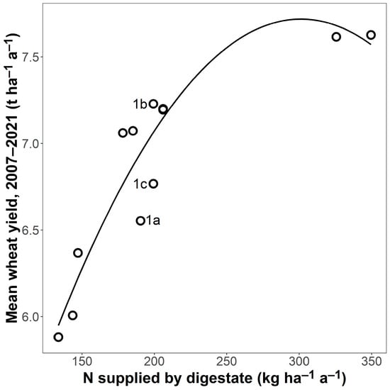
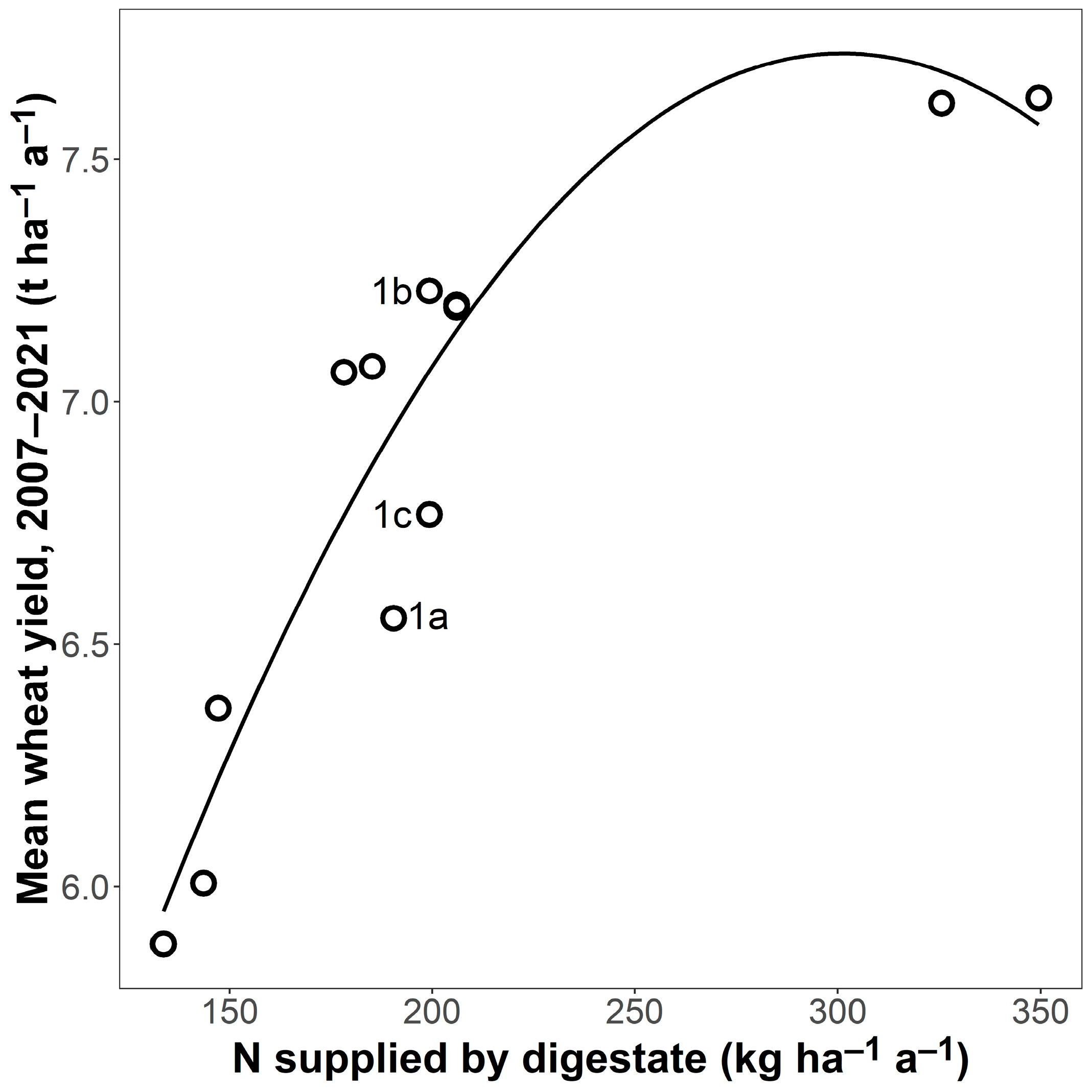
Figure 1.
Wheat grain yield of fertilised plots in relation to N supplied by digestate, average for each crop rotation (n = 12; 10 different crop rotations with three replicates of CR1; CR1 a, b, and c are indicated by their letters). Wheat yield and N supply are mean values of four replicates for the entire experimental period. The line is a regression (y = 2.00 + 0.04 x − 6.31 × 10⁻⁵ x²; R² = 0.87 ***, n = 12).
Yields in the fertilised plots showed a pronounced spatial pattern, with yields higher in CRs in the middle of the field trial than at either end (Figure 2). There was, however, also a positive relationship between field position and digestate N supply (R² = 0.44 *), indicating that those CRs receiving higher amounts of digestate had been placed more towards one end of the field. This was mainly due to the high N supply of over 300 kg ha−1 a−1 in positions 10 and 11. Excluding these two CRs meant the relationship with position was no longer significant (R² decreased to 0.32). The relationship between position and N supply could not, however, explain why yields were higher in the fertilised plots of CR1b (7.23 t ha−1 a−1, 95% CI [6.86, 7.60]) situated in the middle of the experiment than in identically fertilised 1c (6.77 t ha−1 a−1, 95% CI [6.43, 7.10]) and 1a (6.55 t ha−1 a−1, 95% CI [6.02, 7.08]) situated at either end of the field trial (see also Figure 1). Further, the positive relationship between field position and digestate supply did not explain why the unfertilised plots also had the same spatial pattern (CR1b: 4.93 t ha−1 a−1, 95% CI [4.63, 5.23], CR1c: 4.43 t ha−1 a−1, 95% CI [4.09, 4.77], CR1a: 4.00 t ha−1 a−1, 95% CI [3.58, 4.42]). Regression analysis showed that field position was a good predictor of the mean wheat yield, particularly for the unfertilised plots (R² = 0.89 *** unfertilised, 0.60 * fertilised; n = 12 in both cases; Figure 2) and that the relationship with field position was very similar for both the unfertilised and fertilised plots, differing mainly in terms of the intercept (unfertilised: y = 3.48 + 0.36 x − 0.02 x², fertilised: y = 5.70 + 0.30 x − 0.01 x²).
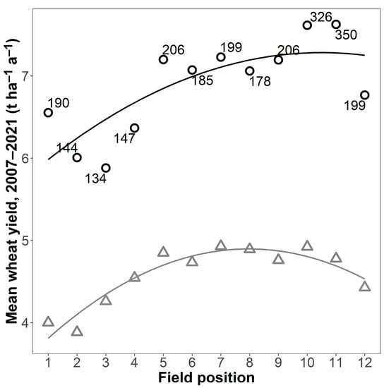
Figure 2.
Wheat yield in fertilised (black circles) and unfertilised plots (grey triangles) in relation to the position of the crop rotation within the experimental area, mean for four replicates for the experimental period. Lines are second-degree polynomial regressions (R² = 0.60 * for the fertilised plots and R² = 0.89 *** for the unfertilised plots). The number next to a point is the mean N supplied by digestate (kg ha–1 a–1, fertilised plots only). Field position is in the same order as crop rotation in Table 1.
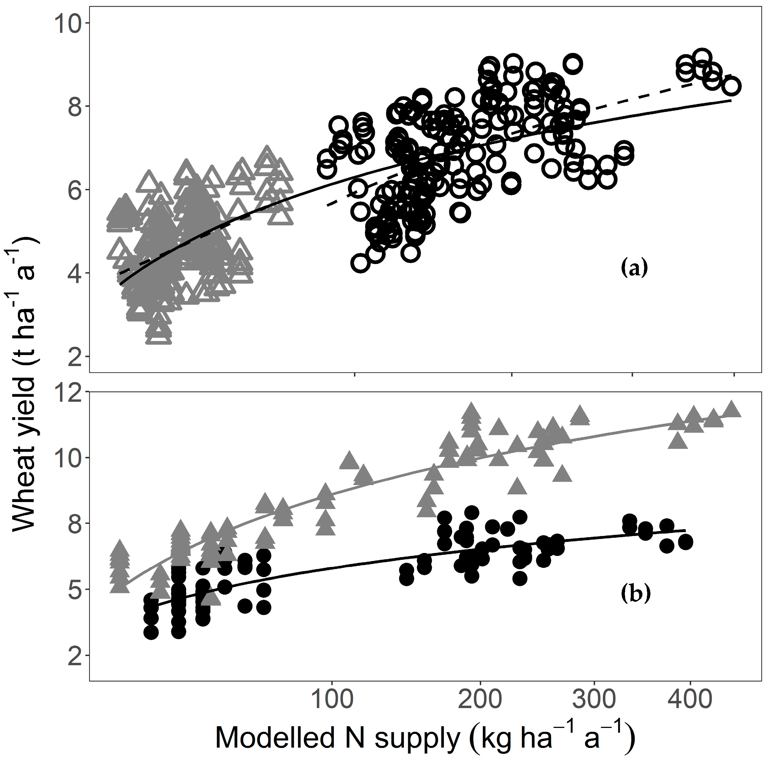
We used our NH3 volatilisation model to test if this spatial pattern had been induced by the experiment itself, using the yield and N supply means for each plot. Yields in the unfertilised plots correlated very highly significantly with the N supplied by neighbouring fertilised plots (R² = 0.25 ***, n = 192). Yields in the fertilised plots also correlated very highly significantly with N supply when losses and gains according to our model were taken into account (R² = 0.31 ***, n = 192). Combining both groups yielded R² = 0.66 *** (n = 384, Figure 3a). Importantly, yields from both fertilised and unfertilised plots showed practically the same response to N supply calculated using our model, even though the slope for the fertilised plots was slightly steeper than the overall slope. Yield response in the unfertilised plots was linear, whereas the overall yield and yield in the fertilised plots had a logarithmic relationship with N supply. This implied that the yield response declined with increasing N supply. Up to an N supply of approximately 200 kg ha−1 a−1, the mean yield response was about 15 kg kg−1, whereas the yield response was only about 5 kg kg−1 for an N supply between 200 to 400 kg ha−1 a−1. This logarithmic relationship was also evident for different years using our model, even though yield levels in these years varied. For example, 2014 was a high-yielding year (mean yield for all plots, fertilised and unfertilised: 8.36 t ha−1 a−1, 95% CI [7.93, 8.80]), and 2010 was a low-yielding year (mean yield for all plots, fertilised and unfertilised: 5.75 t ha−1 a−1, 95% CI [5.51, 5.98]). Nevertheless, the yield-N supply curves for both years show a logarithmic relationship (Figure 3b). For 2010, the regression line had the equation y = ln(x) + 1.04 (R² = 0.69 ***, n = 96), and for 2014, the regression line had the equation y = 2.01 ln(x) − 0.64 (R² = 0.86 ***, n = 95).

Figure 3.
Wheat grain yield in relation to N supply assuming 50% NH3 loss from the fertilised plots to their neighbour plots. All lines are logarithmic regressions (for details of the equations, see text). The x-axis is square-root scaled to improve resolution at low N supply levels. (a) Yield of all 384 plots averaged over three or four years (solid line; R² = 0.66 ***). Fertilised plots are black open circles (upper dashed line: n = 192; R² = 0.31 ***) and unfertilised plots are grey open triangles (lower dashed line: n = 192; R² = 0.25 ***); (b) Comparison of a high-yield year (2014; solid grey triangles; n = 96, R² = 0.86 ***) and a low-yield year (2010; solid black circles; n = 95; R² = 0.69 ***).
Growing conditions in each year had a large influence on yield. This was mainly due to precipitation and, as a result, R² dropped from 0.66 to 0.46 when data from individual years were used instead of multi-year averages (while n increased from 384 to 1221). Precipitation from April to July, the main wheat growth period, ranged from 260 mm (2015) to 464 mm (2021) and was the best simple parameter describing growing conditions. Yields increased linearly with precipitation from April to July for both the fertilised and the unfertilised plots (R² = 0.02 *** for n = 1317). The best combination of the influence of precipitation and N supply was hence given by Y = −1.70 + 0.01 × P + 1.29 ln(N) (R² = 0.49 ***, n = 1221), where Y is wheat yield in t ha−1 a−1, P is precipitation from April to July in mm and N is N supply in kg ha−1 a−1 (see Figure A5 in the Appendix A for a depiction of the regression). Omitting the year 2012, during which a different, low-yielding variety was grown, increased R² to 0.54 *** while n decreased to 1125 with little change in the equation. The multiple regression indicated that the effect of N fertilisation was independent of precipitation, while yields in all plots were higher when precipitation was higher during the growing period.
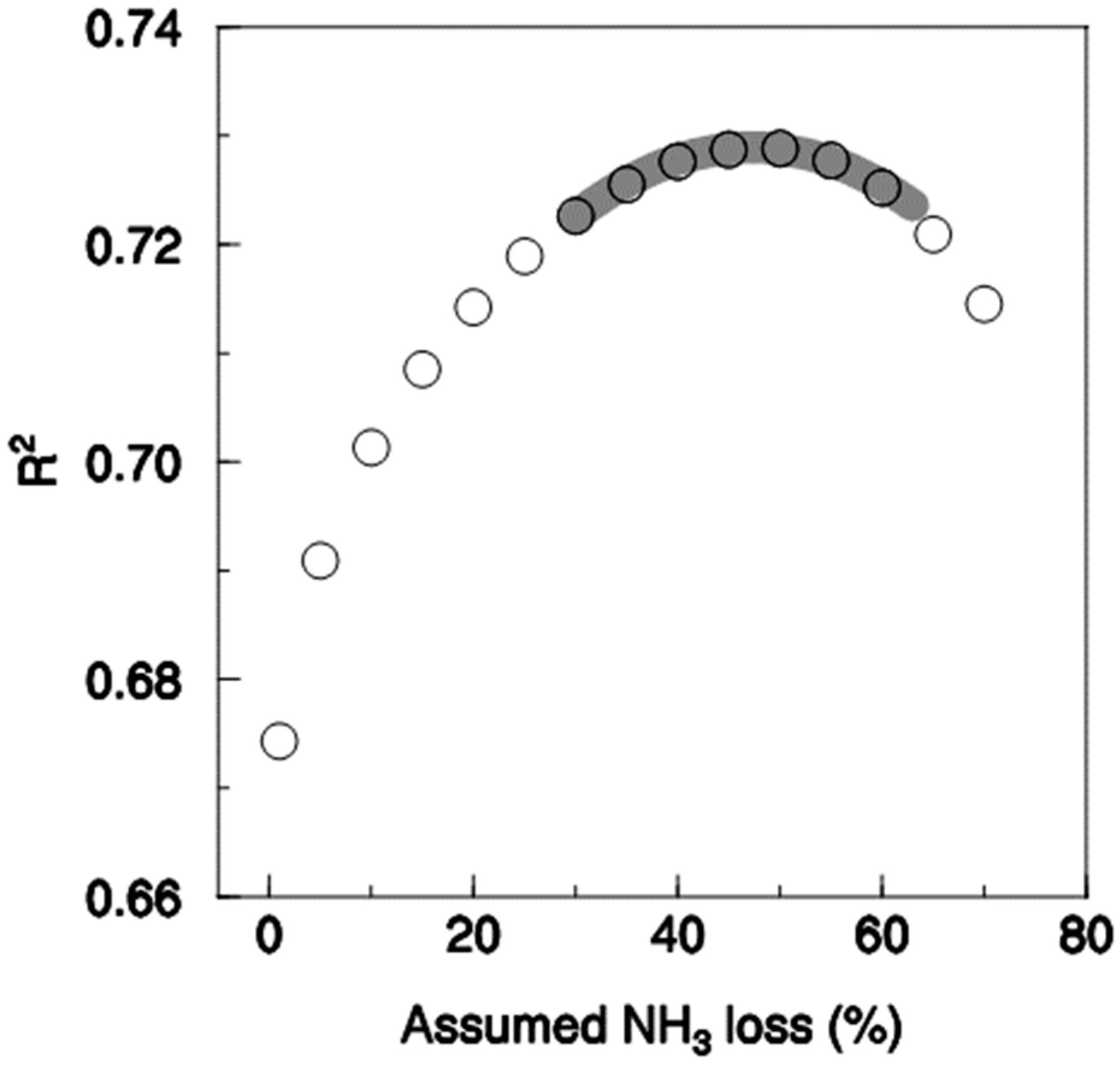
When the fraction of NH4+-N in the digestate transferred to neighbour plots was varied, the highest correlation and a very highly significantly steeper slope of response were found when a loss of 57% was assumed. The coefficient of determination, however, was not significantly different from the peak at 57% when losses ranging from about 30% to almost 70% were assumed (Figure 4). It is, therefore, not possible statistically to say which assumption is best within this range. In contrast, assumed losses below 30% and above 70% were significantly inferior. Assuming no NH3 transfer between plots was the least suitable assumption.

Figure 4.
Coefficient of determination between multi-annual mean wheat grain yield and N supply (n = 384) depending on the assumed NH3 loss of the fertilised plots. The grey line indicates the range where the coefficient of determination is not significantly lower than the maximum at an NH3 loss of 57%, according to the Hotelling test.
PFS measurements showed that ammonia concentrations peaked the day after digestate fertilisation (Figure 5a). In 2021, this peak was seen at all measurement sites, including at a distance of 130 m from the fertilisation site (Figure 5a). In 2022, this peak was seen in both measurement directions (Figure 5b). Ammonia concentrations in fertilised plots (distance = 0) were as high as 40.4 ppm. However, the highest ammonia concentration of 58.0 ppm was measured in a plot directly neighbouring a fertilised plot (position C4, 15 March 2022). Ammonia concentrations were highest in rows C and D, while row A had the lowest ammonia concentrations.
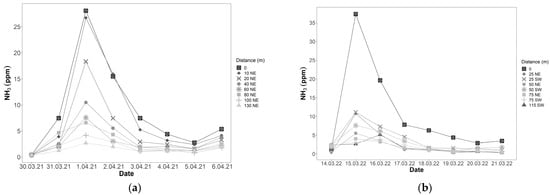
Figure 5.
Average ammonia concentrations measured using the PFS method. Distance is the distance in metres and direction along the field of a PFS measurement site from the fertilised plots (n = 4, NE = northeast, SW = southwest). (a) Ammonia concentrations in 2021. Fertilisation with digestate took place on 31 March 2021; (b) Ammonia concentrations in 2022. Fertilisation with digestate took place on 14 March 2022.
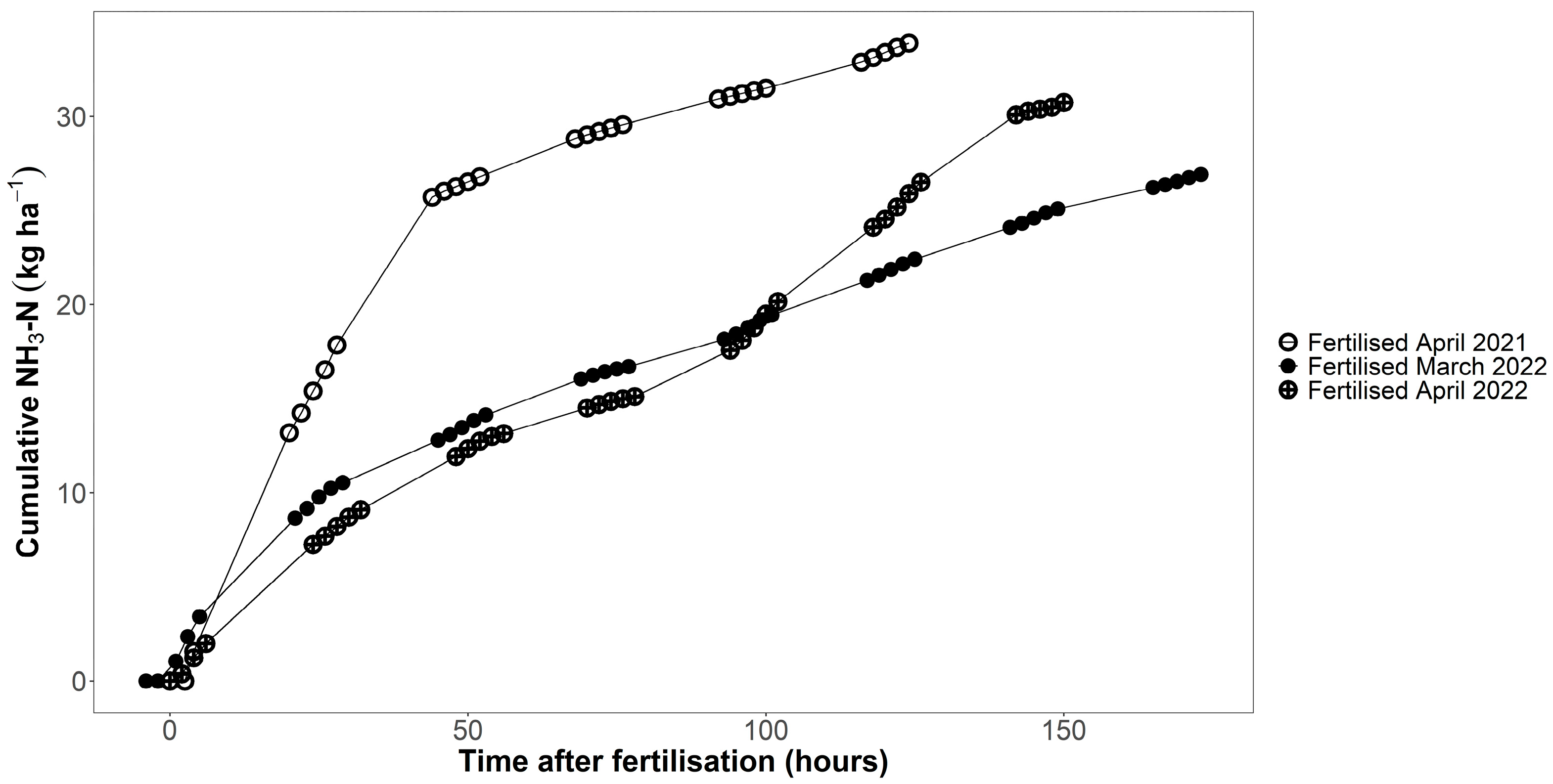
Ammonia measurements using the DTM method showed that the fertilised plots emitted between 24.5 and 37.4 kg ha−1 of ammonia during the measurement period (Figure 6; up to 124 h after fertilisation in 2021, 173 h after fertilisation in the first measurement in 2022, and 150 h in the second measurement in 2022). In 2021, the mean cumulative ammonia emissions 124 h after fertilisation were 33.9 kg ha−1 (n = 6), 56% of the NH4+-N applied to the plots with the digestate. In 2022, mean cumulative ammonia emissions were, on average, 53% of the NH4+-N that had been applied with the digestate. Even though the measurement period was much shorter in 2021 than in 2022, cumulative losses were higher in 2021 than in 2022 (Figure 6). The average temperature during the measurement period in 2021 was 11.5 °C, which was 2–3 °C higher than during the measurement periods in 2022.
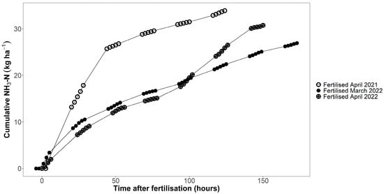
Figure 6.
Cumulative ammonia losses measured in fertilised plots using the DTM method. Fertilisation with digestate took place on 29 April 2021, 14 March 2022 and 28 April 2022 (n = 6).
The emissions from the fertilised plots increased the background concentrations above the unfertilised plots. For example, after fertilisation in April 2021, the NH3 concentrations in the fertilised plots decreased, with a half-life of 19.8 h from 5 ppm 2.5 h after the fertilisation event to 0.3 ppm 124 h after the event (y = 6.7 exp(−0.035 t); n = 54; R² = 0.78). This caused the background NH3 concentrations, as measured above the unfertilised plots, to be as high as 0.25 ppm after the fertilisation event and to fall below the detection limit after 21 h (y = 0.3 exp(−0.065 t); n = 6; R² = 0.99; half-life 10.7 h).
The isotope measurements showed that the grass biomass in the fertilised clover–grass plot had a δ15N value of 6.20‰ and was, therefore, enriched in 15N compared to grass in the unfertilised clover grass plots (Table A2). 15N in grass biomass of the unfertilised plots increased with increasing distance from a fertilised clover–grass plot (Table A2), indicating that the plots further away from the fertilised plot took up less gaseous NH3 than the plots closer to the fertilised plot.
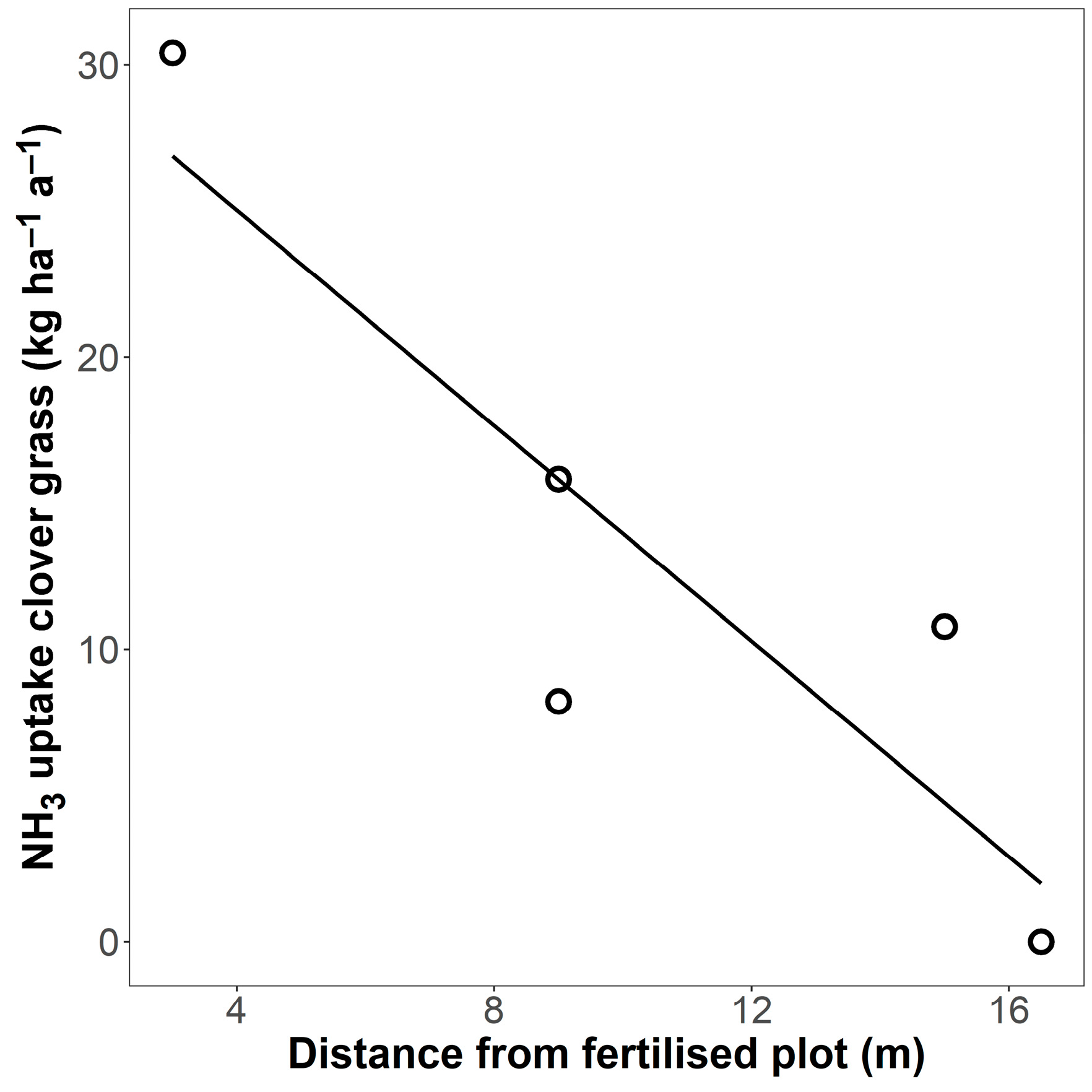
The fraction of total N content in grass biomass originating from NH3 emissions was calculated to be as high as 0.068 (6.8%) in the plot closest to the fertilised plot (Table A2). This fraction decreased with increasing distance from the fertilised plot. Based on these proportions, the plot closest to the fertilised plot was calculated to have taken up 30 kg ha−1 a−1 from NH3 emitted from neighbouring fertilised plots (Figure 7).

Figure 7.
Estimate of gaseous NH3 uptake (kg ha–1 a–1) in five clover–grass plots depending on their distance from a fertilised clover–grass plot, based on 15N isotope measurements. The line is a linear regression (R2 = 0.78 *).
4. Discussion
As expected, digestate fertilisation increased wheat yields and N content when compared with an unfertilised control in accordance with the literature (e.g., [21]), but there was a pronounced spatial pattern in both the fertilised and the unfertilised plots. As soil analyses showed no marked differences in soil properties such as Norg content and field capacity across the site [35], the large number of plots and years and the close correlation over all treatments, especially within the unfertilised plots, leaves little doubt that N transfer between neighbouring plots occurred. Our ammonia emission measurements supported this premise, showing that approximately 55% of the NH4+-N that had been applied with the digestate in our experiment was volatilised within a few days, with these ammonia emissions being transported at least as far as 130 m from the original site of fertilisation, and in different directions along the experimental field. Ammonia concentrations were highest at or in the immediate vicinity of the fertilisation site. This was reflected by the 15N isotope analysis, where δ15N was highest in grass biomass in the fertilised plot and lowest in grass biomass in the plots neighbouring the fertilised plot, increasing again in plots further away from the fertilised plot. This indicated that the grass biomass in the fertilised plot had taken up NH4+-N directly from the digestate. In contrast, grass biomass in the unfertilised plots absorbed 15N-depleted NH3-N volatilised from the digestate, with grass biomass in plots neighbouring the fertilised plot absorbing more than grass biomass in plots further away from the fertilised plot. We expect that isotope measurements at greater distances from the site of fertilisation would also indicate these effects. The size of these effects will depend on the prevailing wind direction and wind speed at the site. For example, Boaretto et al. [36] observed variation in the absorption of 15NH3 in citrus trees equidistant from the fertilisation site, presumably due to wind direction. In an orchard protected from the wind, coffee plants reabsorbed 43% of the volatilised NH3-N [37].
In principle, processes other than NH3 volatilisation could have contributed to the spatial pattern seen in the experiment. In particular, N in subsurface water flow may be important [10,38,39]. This would, however, only have caused an N transfer downslope while the plots upslope would not have been affected. This would have split the unfertilised plots into two groups, one group with consistently low yields, even in cases where our simple modelling assumed large N transfers from neighbouring plots, while the other group should have responded to digestate application in the fertilised plot in the upslope position. Such a split in the data was not evident. Furthermore, NH3 volatilisation can explain all the effects that we see in our study. In particular, this explained why CR1a and c, situated at the outer edges of the experiment, had lower yields than CR1b, despite identical treatment. It even explained why CR1c, located next to a CR receiving the highest amounts of digestate-N, had a higher yield than CR1a, which was situated next to CRs receiving the lowest amounts of digestate-N. It explained why, for both the fertilised and the unfertilised plots, the relationship of yield with position was a parabola with the highest yields in the positions in the middle where NH3 import from both sides was possible, whereas the lowest yields occurred at both edges where import was possible only from one side. N balances calculated for the unfertilised plots show large N deficits [40] without a correspondingly large decrease in yields with time. N transfer via NH3 volatilisation would explain this effect.
Plot experiments usually aim at minimizing soil heterogeneity to reduce statistical error. This can best be achieved by using small plots and situating treatments in close proximity to each other. In addition, strong gradients between treatments are desirable for producing detectable effects. Both experimental design strategies become undesirable if the NH3 flow between treatments should be kept at a minimum. The inference from our experiment is that such experiments should use much larger plots with a larger area-to-circumference ratio, and treatments should be separated by larger distances. The average plot size in wheat fertiliser trials is 37.2 m2 [41], which is only half the size of the plots in our experiment. The effects would, therefore, normally be even more pronounced. A completely different experimental layout to what is traditionally used would also avoid the inherent problem with traditional designs, which is that replicates are actually pseudoreplicates [42] because they all investigate the same conditions, i.e., soil, weather and microclimate, and, thus, generalization of the results to a wider variety of settings is not possible.
The mean field size in the region where the experiment was situated is 5.7 ha [43], which is three orders of magnitude larger than the typical plot size or the plot size in our experiment. Therefore, the question arises as to which group of plots was more affected by the experimental design, fertilised or unfertilised, and, thus, which result differs more from the response that would occur in farmers’ fields. The very flat increase in yield with increasing N in the fertilised plots means that in large fields, the increase in yield may be higher if losses are lower because of a large area-to-circumference ratio. This effect, however, may not be large because there would be no NH3 sink in the field if the entire crop has reached the stomatal ammonia compensation point after a fertilisation event. Long-distance losses would then result. The steep gradient of the curve for the unfertilised plots indicates that they profit strongly from their fertilised neighbours, but only if such neighbours exist. In farmers’ fields, this may only be true at the field edge. In addition, the timing may be less favourable than in our experiment, where a wheat plot was situated beside a wheat plot, and thus emissions from neighbouring plots occurred at a time when a large fertilisation effect for wheat was expected. Such a perfect match will not always be the case in reality. For both reasons, the trapping effect of unfertilised fields will also be smaller in reality, which again would favour long-distance losses. It is, thus, unfortunate that there is a strong trend in modern agriculture of increasing field sizes [44,45,46], which will increase regional-scale NH3 emissions and decrease the applicability of results from small-plot experiments. An N surplus causes a shift in δ15N at the farm level, indicative of emissions at a regional scale, rather than field-to-field transfer of NH3 [47,48].
An even more important question is which measures could, therefore, be taken in agriculture to reduce NH3 losses. The estimated loss of 57% that performed best in our model was corroborated by our ammonia emission measurements and was similar to the German emission factor for NH3 for the application of cattle slurry and digestate derived from cattle slurry using trailing hoses without incorporation (46%) [49], and is, therefore, not unrealistic. The reasoning above means that losses would also occur in large plots and hence, also in fields. We found a consistent effect in many plots and over many years that was even more pronounced in dry years than in wet years. This makes it likely that it will occur under many conditions. Such a consistent effect would not be very likely if it were only caused by the conditions during fertiliser application, which must have varied considerably over the long experimental period. In addition, an N supply above 200 kg ha−1 had barely any effect on yields, with our data indicating that at N supply levels above 280 kg ha−1, wheat yields may start to decrease. Other authors have found similar effects in wheat [50]. This means that the high N inputs could have increased the apoplastic NH4+ concentration in the wheat crop, thereby increasing the NH3 compensation point and causing NH3 emission [15,51]. Therefore, even incorporation of the digestate into the soil would not prevent NH3 losses to the environment, and the same amount of mineral fertiliser could also induce foliar NH3 losses [52,53,54]. Splitting fertilisation into two applications would also not have a large effect, as indicated by the flat relationship between N supply and yield. It appears that the best way of reducing NH3 losses would be a slow-release N source that does not cause peaks in the stomatal NH3 compensation point. Easily degradable carbon compounds are decomposed during the anaerobic digestion process [4]; thus, liquid animal slurries contain more organic matter than digestates and should deliver N more slowly than digestates. Solid manures should be even better in this regard than liquid manures. In the short term, crop N utilization of solid manures and the resulting yields are often the same or lower than for liquid manures or mineral N fertilisers [55,56]. However, in the long term, solid manures show a substantial increase in N utilization [57]. For example, Paul and Beauchamp [58] found that the N availability from composted manure was as high during the third year after a one-off application as in the first year. While these results are often attributed to improvements in soil structure and increases in organic matter stimulating soil fertility over time [55], our results indicate that higher N-use efficiencies may also be due to lower foliar N losses with slow-release N fertilisers. Möller and Stinner [4], for example, found that ammonia emissions were lower after the application of solid farmyard manure than after the application of slurry or digestate. However, total canopy NH3 emission or deposition depends not only on emission/deposition fluxes from plant stomata and cuticles but also on fluxes from soil and litter and the interactions between these different components and with atmospheric NH3 concentrations [59]. Soil emission potentials are significantly larger than the stomatal emission potentials, and the soil is, therefore, likely to have the biggest influence on total canopy emissions [60,61].
Our simple model, which explained all data well irrespective of whether we looked at high-yield years or low-yield years or whether we looked at fertilised or unfertilised plots, implies that the availability and the effects on yield are identical for NH3-N and for other, mainly organic N sources, in the digestate. The relationships described above would disappear if we assumed only NH3-N or only organic N was available and responsible for our results. It is generally assumed that mineral N (NO3− and NH4+ ions) is immediately available for plant uptake, whereas organic matter first has to be mineralised before organic N pools can be used by plants [62,63,64]. The apparently high availability and effectiveness of the organic N were not due to an accumulation in the soil organic matter pool and subsequent slow release, which is likely to occur in a long-term experiment. If this were the case, the effect of the organic N should have increased with time. This was not evident in our field trial. In particular, in the comparison of yields from 2010 (four years after the first fertilisation) and 2014, there was no offset of the plots receiving organic N from the digestate that could be attributed to increased N release from a pool of soil organic N that had accumulated over time. The differences between years were only caused by the different weather conditions and appeared in both the plots that had received organic N and the plots that did not receive organic N. In the long term, N losses in this field trial may increase as N in the soil organic matter pool reaches a stable level and no longer accumulates, but N is still added via digestate fertilisation. This is particularly the case for CRs 9 and 10, both CRs with a high proportion of clover–grass, and, therefore, additional N fixation, that have built up large soil organic matter stocks over the experimental period [65,66].
In our experiment, the decreasing effectiveness of N with increasing N supply indicated that losses of NH3 (presumably mainly long-distance aerial transport) and organic N (presumably mainly leaching and denitrification losses) were similar for both N sources. This may not be the case at other sites. Soil type may have an effect, for example. In particular, in a considerably drier and warmer climate, NH3 losses would probably have been higher, and leaching and denitrification losses would probably have been lower. The net effect, however, should be low because both changes cancel each other out.
5. Conclusions
Analysing more than a decade of yields on 384 plots and using a simple N loss/gain model enabled us to see how NH3 emissions from plots fertilised with biogas digestate affected yields in neighbouring unfertilised plots and to understand the availability of N from biogas digestate. Ammonia volatilisation measurements and 15N isotope analysis to investigate shoot N absorption validated the results of the model. Our results have important implications, not only for the interpretation of plot experiments but also for agricultural practise. Our results indicate that in order to avoid inadvertently affecting unfertilised control plots, plot sizes need to be increased and treatments situated further apart. Foliar NH3 emissions and, therefore, agricultural ammonia emissions in general may be reduced if solid rather than liquid organic manures are used; however, the effect of solid manures on the ammonia compensation point of crops needs further investigation. Further investigation in general is needed on how organic fertilisers affect the various components contributing to the overall emission or deposition of NH3 in agricultural crops. It appears that the organic N in the biogas digestate used in our field trial was highly crop-available, and therefore, there was also a high risk of N losses. Further research on the availability of organic N from digestates is needed to confirm our findings.
Author Contributions
Conceptualization, K.A. and K.S.L.; methodology, K.A.; validation, K.A.; formal analysis, K.S.L., K.A. and F.W.; investigation, H.J.R., F.W. and K.S.L.; resources, K.-J.H.; data curation, K.S.L. and F.W.; writing—original draft preparation, K.S.L.; writing—review and editing, K.A., K.S.L. and F.W.; visualization, K.S.L. and K.A.; supervision, K.A., H.J.R. and K.-J.H.; project administration, H.J.R. and K.-J.H.; funding acquisition, H.J.R. and K.-J.H. All authors have read and agreed to the published version of the manuscript.
Funding
Ammonia measurements took place as part of the MASTER project, grant number 22025917, funded by the German Federal Office for Agriculture and Food. Data collection in the field trial for the period 2013–2016 was funded by the Bavarian State Ministry of Food, Agriculture and Forestry as part of the project BOFRUBIOGAS, grant number A 13/17. The Technical University of Munich Publishing Fund provided funding for the publication of this article.
Institutional Review Board Statement
Not applicable.
Data Availability Statement
The data presented in this study are available on request from the corresponding author.
Acknowledgments
The authors would like to thank Stefan Kimmelmann, Florian Schmid and Horst Laffert for their hard work over many years managing the field trial and collecting data. The authors would also like to thank Rudi Schäufele from the TUM School of Life Sciences for the isotope measurements, and Max Kainz for designing the experiment. K.S.L. and F.W. would also like to acknowledge the support of the TUM Graduate School (Graduate Center of Life Sciences).
Conflicts of Interest
The authors declare no conflict of interest. The funders had no role in the design of the study; in the collection, analyses, or interpretation of data; in the writing of the manuscript; or in the decision to publish the results.
Appendix A
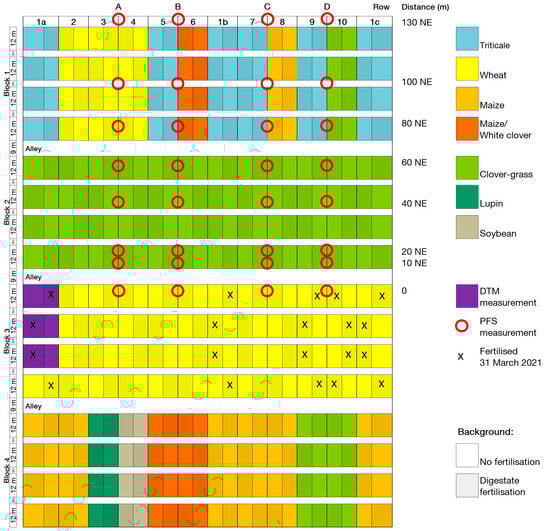
Figure A1.
Plot and ammonia volatilisation measurement plan 2021. Row refers to the PFS measurement row, distance is the distance in metres and the direction along the field of a PFS measurement site from the fertilised plots (NE = northeast), red circles indicate the location of the PFS measurement sites, X marks the plots that were fertilised with digestate on 31 March 2021 during PFS measurement. DTM measurements took place in the plots coloured purple.
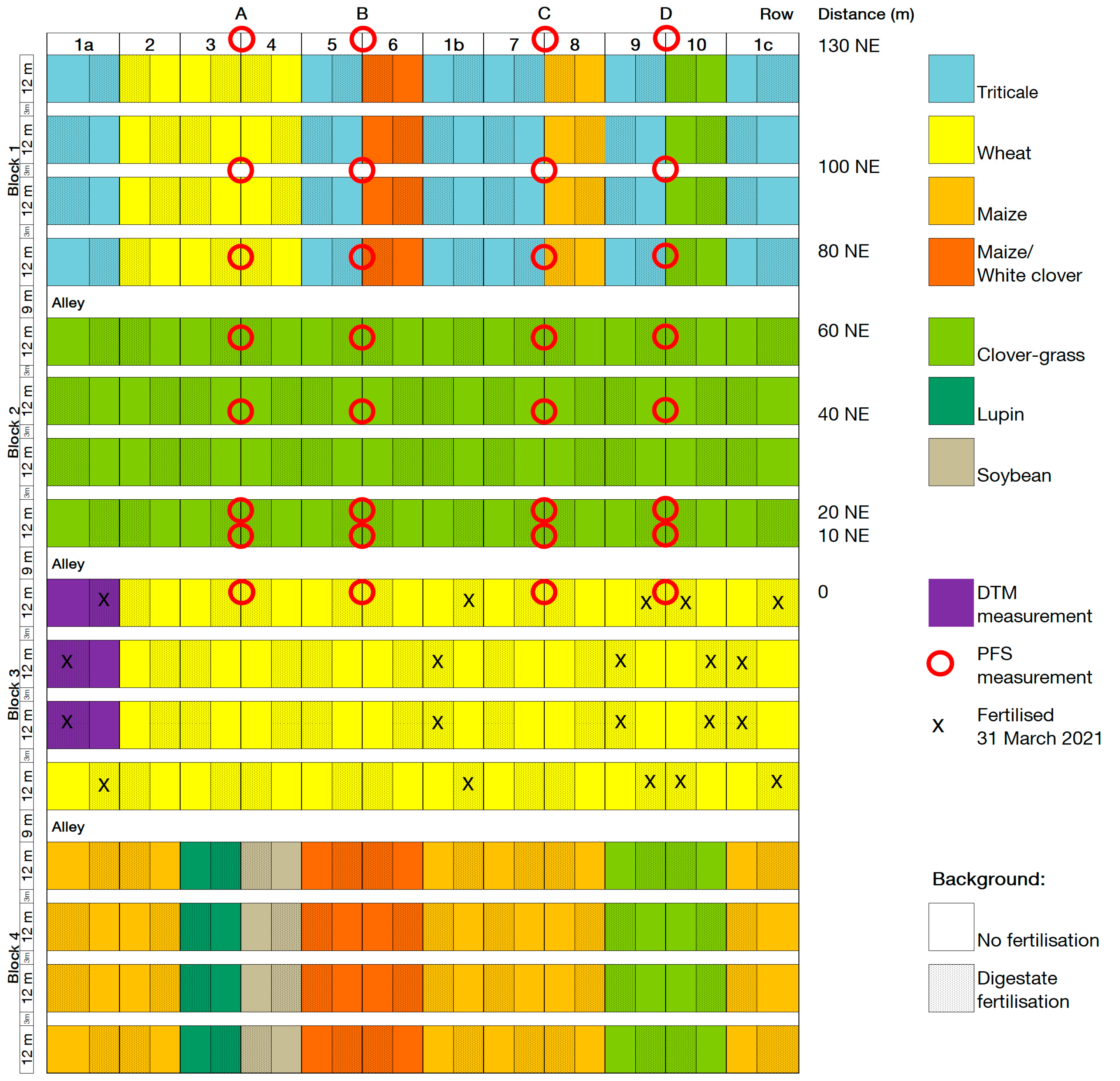
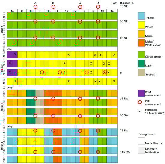
Figure A2.
Plot and ammonia volatilisation measurement plan 2022. Row refers to the PFS measurement row, distance is the distance in metres and direction along the field of a PFS measurement site from the fertilised plots (NE = northeast, SW = southwest), red circles indicate the location of the PFS measurement sites, X marks the plots that were fertilised with digestate on 14 March 2022 during PFS measurement. DTM measurements took place in the plots coloured purple.
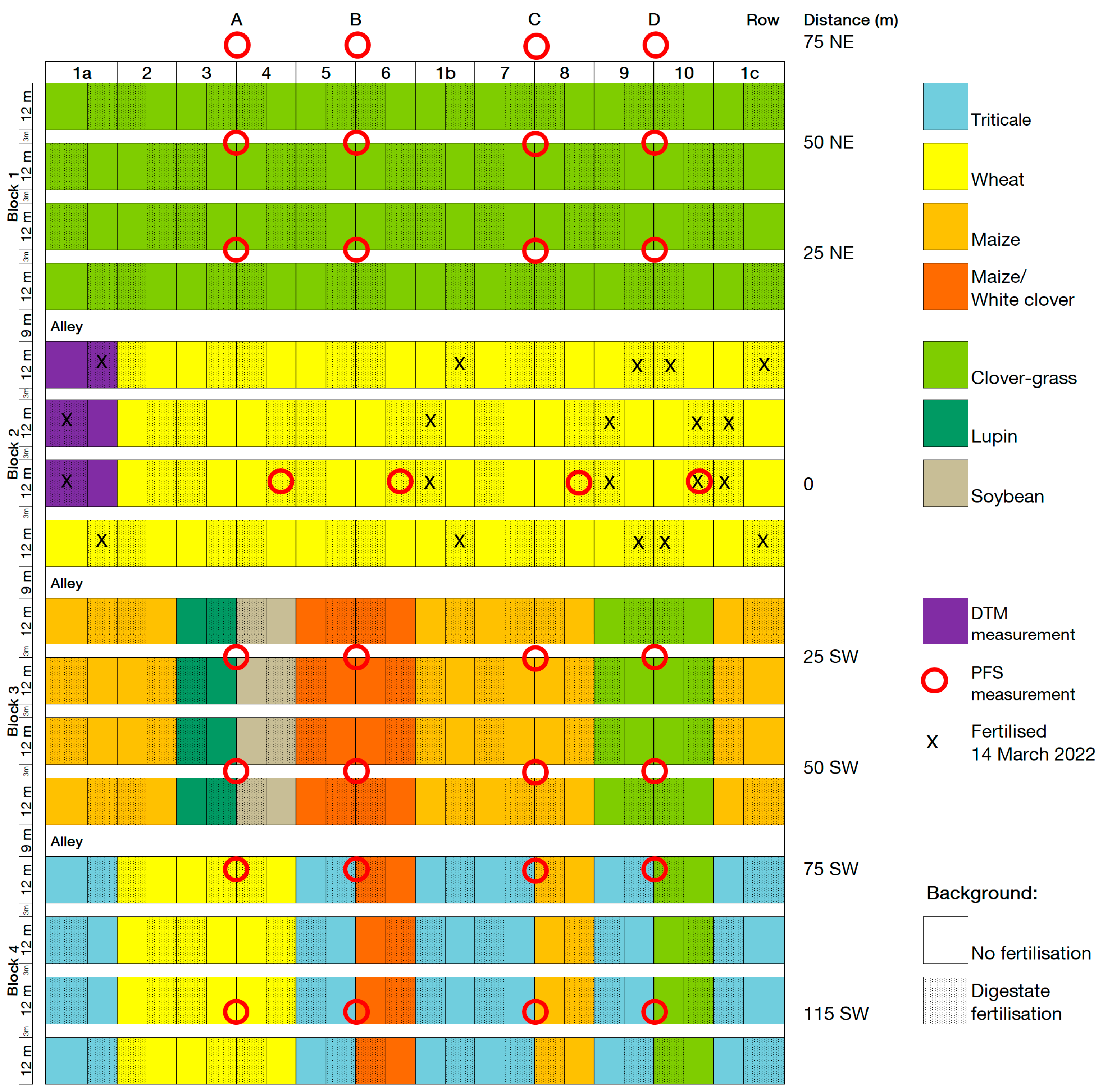

Figure A3.
Ammonia measurement using the DTM method in a fertilised wheat plot.
Figure A3.
Ammonia measurement using the DTM method in a fertilised wheat plot.
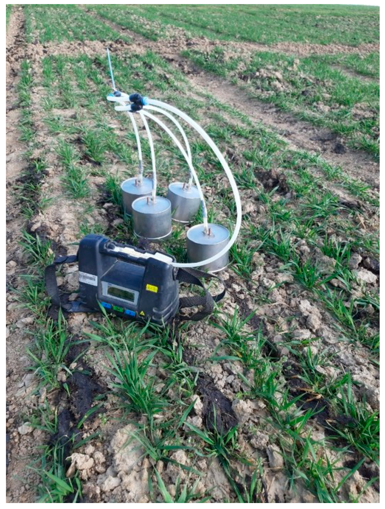
Table A1.
Weather conditions during ammonia measurements in 2021 and 2022.
Table A1.
Weather conditions during ammonia measurements in 2021 and 2022.
| Date | Mean Temperature (Daily, °C) | Mean Temperature (During DTM Measurement, °C) | Mean Wind Speed (Daily, m s−1) | Mean Wind Speed (During DTM Measurement, m s−1) | Wind Direction | Mean Pressure (During DTM Measurement, hPa) |
|---|---|---|---|---|---|---|
| 30 March 2021 | 12.7 | 0.9 | ESE | |||
| 31 March 2021 | 13.4 | 1 | SSE | |||
| 1 April 2021 | 13.7 | 2 | W | |||
| 2 April 2021 | 8.3 | 3 | NW | |||
| 3 April 2021 | 4.4 | 2.8 | NW | |||
| 4 April 2021 | 5.2 | 1.5 | WNW | |||
| 5 April 2021 | 5.3 | 4.3 | SW | |||
| 6 April 2021 | −0.8 | 3.3 | WSW | |||
| 29 April 2021 | 12.9 | 2.5 | 1007.4 | |||
| 30 April 2021 | 14.1 | 3.3 | 1008.4 | |||
| 1 May 2021 | 10.5 | 2.8 | 1009.1 | |||
| 2 May 2021 | 6.3 | 4.1 | 1017.6 | |||
| 3 May 2021 | 10.0 | 3.1 | 1021.6 | |||
| 4 May 2021 | 16.0 | 4.9 | 1007.7 | |||
| 14 March 2022 | 8.2 | 12.1 | 2.3 | 2.1 | WSW | 1028 |
| 15 March 2022 | 7.1 | 8.9 | 1.7 | 1.1 | ENE | 1026.0 |
| 16 March 2022 | 7.1 | 8.9 | 2.8 | 2.6 | E | 1026.4 |
| 17 March 2022 | 6.1 | 7.9 | 1.8 | 1.3 | E | 1027.2 |
| 18 March 2022 | 7.5 | 10.0 | 3.2 | 3.4 | NE | 1036.9 |
| 19 March 2022 | 5.5 | 8.0 | 3.5 | 3.6 | NNE | 1033.7 |
| 20 March 2022 | 6.7 | 10.7 | 2.9 | 3.3 | E | 1031.0 |
| 21 March 2022 | 6.3 | 9.7 | 1.6 | 1.8 | ENE | 1032.8 |
| 28 April 2022 | 14.3 | 2.3 | 1027.2 | |||
| 29 April 2022 | 16.1 | 2.6 | 1024.1 | |||
| 30 April 2022 | 12.2 | 2.5 | 1020.7 | |||
| 1 May 2022 | 10.5 | 1.7 | 1020.4 | |||
| 2 May 2022 | 1.7 | 15.6 | 1014.9 | |||
| 3 May 2022 | 2.0 | 16.3 | 1013.7 | |||
| 4 May 2022 | 2.1 | 16.6 | 1015.3 |
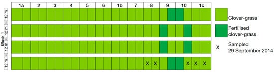
Figure A4.
Plan of clover–grass plots sampled for isotope analysis on 29 September 2014.
Figure A4.
Plan of clover–grass plots sampled for isotope analysis on 29 September 2014.
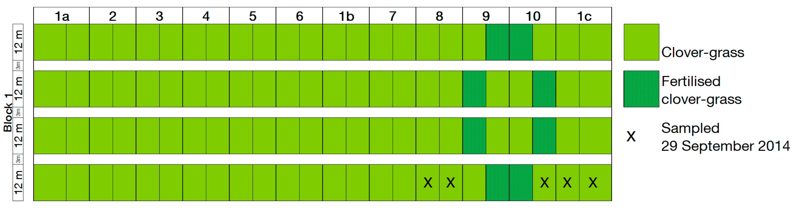

Figure A5.
Multiple regression of wheat grain yield in relation to N supply and precipitation during the main growing period (R² = 0.48 *** for n = 1221).
Figure A5.
Multiple regression of wheat grain yield in relation to N supply and precipitation during the main growing period (R² = 0.48 *** for n = 1221).

Table A2.
δ15N in clover–grass sampled on 29 September 2014.
Table A2.
δ15N in clover–grass sampled on 29 September 2014.
| Distance across the Field from Fertilised Clover–Grass Plot (m) | δ15N Grass Component (‰) | Fraction of Total N in Grass Component Derived from Gaseous NH3 Emissions |
|---|---|---|
| 3 | 1.35 | 0.068 |
| 9 | 1.53 | 0.060 |
| 9 | 2.24 | 0.029 |
| 15 | 2.16 | 0.032 |
| 16.5 | 2.90 | 0 |
References
- Brackin, R.; Näsholm, T.; Robinson, N.; Guillou, S.; Vinall, K.; Lakshmanan, P.; Schmidt, S.; Inselsbacher, E. Nitrogen fluxes at the root-soil interface show a mismatch of nitrogen fertilizer supply and sugarcane root uptake capacity. Sci. Rep. 2015, 5, 15727. [Google Scholar] [CrossRef] [PubMed]
- Raun, W.R.; Johnson, G.V. Improving nitrogen use efficiency for cereal production. Agron. J. 1999, 91, 357. [Google Scholar] [CrossRef]
- Eurich-Menden, B.; Döhler, H.; Dämmgen, U. Ammonia emissions of German agriculture. Landtechnik 2004, 59, 162–163. [Google Scholar] [CrossRef]
- Möller, K.; Stinner, W. Effects of different manuring systems with and without biogas digestion on soil mineral nitrogen content and on gaseous nitrogen losses (ammonia, nitrous oxides). Eur. J. Agron. 2009, 30, 1–16. [Google Scholar] [CrossRef]
- Battye, W.; Aneja, V.P.; Schlesinger, W.H. Is nitrogen the next carbon? Earth’s Future 2017, 5, 894–904. [Google Scholar] [CrossRef]
- Mosier, A.R. Exchange of gaseous nitrogen compounds between agricultural systems and the atmosphere. Plant Soil 2001, 228, 17–27. [Google Scholar] [CrossRef]
- Underwood, A.J. Components of design in ecological field experiments. Ann. Zool. Fenn. 2009, 46, 93–111. [Google Scholar] [CrossRef]
- Petersen, R.G. Agricultural Field Experiments: Design and Analysis; Marcel Dekker, Inc.: New York, NY, USA, 1994; ISBN 0824789121. [Google Scholar]
- Gomez, K.A.; Gomez, A.A. Statistical Procedures for Agricultural Research, 2nd ed.; Wiley: New York, NY, USA, 1984; ISBN 9780471879312. [Google Scholar]
- Jackson, W.A.; Asmussen, L.E.; Hauser, E.W.; White, A.W. Nitrate in surface and subsurface flow from a small agricultural watershed. J. Environ. Qual. 1973, 2, 480–482. [Google Scholar] [CrossRef]
- Vervoort, R.W.; Radcliffe, D.E.; Cabrera, M.L.; Latimore, M., Jr. Nutrient losses in surface and subsurface flow from pasture applied poultry litter and composted poultry litter. Nutr. Cycl. Agroecosystems 1998, 50, 287–290. [Google Scholar] [CrossRef]
- Castro, A.; Stulen, I.; De Kok, L.J. Atmospheric NH3 as plant nutrient: A case study with Brassica oleracea. Environ. Pollut. 2008, 154, 467–472. [Google Scholar] [CrossRef]
- Farquhar, G.D.; Firth, P.M.; Wetselaar, R.; Weir, B. On the gaseous exchange of ammonia between leaves and the environment: Determination of the ammonia compensation point. Plant Physiol. 1980, 66, 710–714. [Google Scholar] [CrossRef] [PubMed]
- Nemitz, E.; Milford, C.; Sutton, M.A. A two-layer canopy compensation point model for describing bi-directional biosphere-atmosphere exchange of ammonia. Q. J. Royal. Met. Soc. 2001, 127, 815–833. [Google Scholar] [CrossRef]
- Asman, W.A.H.; Sutton, M.A.; Schjorring, J.K. Ammonia: Emission, atmospheric transport and deposition. New Phytol. 1998, 139, 27–48. [Google Scholar] [CrossRef]
- Högberg, P. Tansley Review No. 95 15N natural abundance in soil-plant systems. New Phytol. 1997, 137, 179–203. [Google Scholar] [CrossRef]
- Frank, D.A.; Evans, R.D.; Tracy, B.F. The role of ammonia volatilization in controlling the natural 15N abundance of a grazed grassland. Biogeochemistry 2004, 68, 169–178. [Google Scholar] [CrossRef]
- Möller, K.; Müller, T. Effects of anaerobic digestion on digestate nutrient availability and crop growth: A review. Eng. Life Sci. 2012, 12, 242–257. [Google Scholar] [CrossRef]
- Gericke, D.; Bornemann, L.; Kage, H.; Pacholski, A. Modelling ammonia losses after field application of biogas slurry in energy crop rotations. Water Air Soil Pollut. 2012, 223, 29–47. [Google Scholar] [CrossRef]
- Möller, K. Effects of anaerobic digestion on soil carbon and nitrogen turnover, N emissions, and soil biological activity. A review. Agron. Sustain. Dev. 2015, 35, 1021–1041. [Google Scholar] [CrossRef]
- Abubaker, J.; Risberg, K.; Pell, M. Biogas residues as fertilisers—Effects on wheat growth and soil microbial activities. Appl. Energy 2012, 99, 126–134. [Google Scholar] [CrossRef]
- Quakernack, R.; Pacholski, A.; Techow, A.; Herrmann, A.; Taube, F.; Kage, H. Ammonia volatilization and yield response of energy crops after fertilization with biogas residues in a coastal marsh of Northern Germany. Agric. Ecosyst. Environ. 2012, 160, 66–74. [Google Scholar] [CrossRef]
- Wulf, S.; Maeting, M.; Clemens, J. Application technique and slurry co-fermentation effects on ammonia, nitrous oxide, and methane emissions after spreading: I. Ammonia volatilization. J. Environ. Qual. 2002, 31, 1789–1794. [Google Scholar] [CrossRef] [PubMed]
- Ni, K.; Pacholski, A.; Gericke, D.; Kage, H. Analysis of ammonia losses after field application of biogas slurries by an empirical model. J. Plant Nutr. Soil Sci. 2012, 175, 253–264. [Google Scholar] [CrossRef]
- Nyord, T.; Hansen, M.N.; Birkmose, T.S. Ammonia volatilisation and crop yield following land application of solid–liquid separated, anaerobically digested, and soil injected animal slurry to winter wheat. Agric. Ecosyst. Environ. 2012, 160, 75–81. [Google Scholar] [CrossRef]
- Wolf, U. Emission of NH3, N2O and CO2 following the application of differently treated digestates from biogas production. Ph.D. Thesis, Technische Universität Carolo-Wilhelmina zu Braunschweig, Braunschweig, Germany, 2014. [Google Scholar]
- Senbayram, M.; Chen, R.; Mühling, K.H.; Dittert, K. Contribution of nitrification and denitrification to nitrous oxide emissions from soils after application of biogas waste and other fertilizers. Rapid Commun. Mass Spectrom. 2009, 23, 2489–2498. [Google Scholar] [CrossRef]
- Soil Survey Staff. Illustrated Guide to Soil Taxonomy: Version 2.0; USDA: Lincoln, NE, USA, 2015.
- IUSS Working Group WRB. World Reference Base for Soil Resources 2014: International Soil Classification System for Naming Soils and Creating Legends for Soil Maps; FAO: Rome, Italy, 2014; ISBN 978-92-5-108369-7. [Google Scholar]
- Pacholski, A.; Cai, G.; Nieder, R.; Richter, J.; Fan, X.; Zhu, Z.; Roelcke, M. Calibration of a simple method for determining ammonia volatilization in the field—Comparative measurements in Henan Province, China. Nutr. Cycl. Agroecosys 2006, 74, 259–273. [Google Scholar] [CrossRef]
- Pacholski, A. Calibrated passive sampling—Multi-plot field measurements of NH3 emissions with a combination of dynamic tube method and passive samplers. J. Vis. Exp. 2016, 109, e53273. [Google Scholar] [CrossRef]
- Auerswald, K.; Schäufele, R.; Schnyder, H. Paths of nitrogen transfer from Trifolium repens to non-legume plants in unfertilised pastures. In Grassland in a Changing World: Proceedings of the 23th General Meeting of the European Grassland Federation Kiel, Germany, August 29th–September 2nd 2010; Schnyder, H., Isselstein, J., Taube, F., Auerswald, K., Schellberg, J., Wachendorf, M., Herrmann, A., Gierus, M., Wrage, N., Eds.; Mecke Druck und Verlag: Duderstadt, Germany, 2010; pp. 752–754. ISBN 978-3-86944-021-7. [Google Scholar]
- R Core Team. R: A Language and Environment for Statistical Computing; R Foundation for Statistical Computing: Vienna, Austria, 2022. [Google Scholar]
- Hotelling, H. The teaching of statistics. Ann. Math. Stat. 1940, 11, 457–470. [Google Scholar] [CrossRef]
- Simon, A.I.L. Langzeitwirkungen von Gärresten in Energiepflanzenfruchtfolgen auf Bodeneigenschaften und Bodenprozesse unter den Bedingungen des ökologischen Landbaus, 1. Auflage; Verlag Dr. Köster: Berlin, Germany, 2021; ISBN 9783968310138. [Google Scholar]
- Boaretto, R.M.; Mattos, D., Jr.; Quaggio, J.A.; Cantarella, H.; Trivelin, P.C.O. Absorption of 15NH3 volatilized from urea by Citrus trees. Plant Soil 2013, 365, 283–290. [Google Scholar] [CrossRef]
- Bergamo Fenilli, T.A.; Reichardt, K.; Ocheuze Trivelin, P.C.; Favarin, J.L. Volatilization of ammonia derived from fertilizer and its reabsorption by coffee plants. Commun. Soil Sci. Plant Anal. 2007, 38, 1741–1751. [Google Scholar] [CrossRef]
- Randall, G.W.; Mulla, D.J. Nitrate nitrogen in surface waters as influenced by climatic conditions and agricultural practices. J. Environ. Qual. 2001, 30, 337–344. [Google Scholar] [CrossRef]
- Sharpley, A.N.; Syers, J.K. Amounts and relative significance of runoff types in the transport of nitrogen into a stream draining an agricultural watershed. Water Air Soil Pollut Water Air Soil Pollut. 1981, 15, 299–308. [Google Scholar] [CrossRef]
- Reents, H.J.; Simon, A.; Levin, K.; Hülsbergen, K.-J. Wirkungen von Biogassystemen auf Bodenfruchtbarkeit, Ertrag und Produktqualität unter den Bedingungen des ökologischen Landbaus: BOFRUBIOGAS; Project Report; Bavarian State Ministry for Food, Agriculture and Forestry: Munich, Germany, 2018.
- Taylor, S.L.; Payton, M.E.; Raun, W.R. Relationship between mean yield, coefficient of variation, mean square error, and plot size in wheat field experiments. Commun. Soil Sci. Plant Anal. 2008, 30, 1439–1447. [Google Scholar] [CrossRef]
- Hurlbert, S.H. Pseudoreplication and the design of ecological field experiments. Ecol. Monogr. 1984, 54, 187–211. [Google Scholar] [CrossRef]
- Auerswald, K.; Fischer, F.K.; Kistler, M.; Treisch, M.; Maier, H.; Brandhuber, R. Behavior of farmers in regard to erosion by water as reflected by their farming practices. Sci. Total Environ. 2018, 613–614, 1–9. [Google Scholar] [CrossRef]
- Ankenbrand, E.; Schwertmann, U. The land consolidation project of Freinhausen, Bavaria. In Soil Erosion Protection Measures in Europe, Proceedings of the European Community Workshop on Soil Erosion Protection, Freising, Federal Republic of Germany, 24–26 May 1988; Schwertmann, U., Rickson, R.J., Auerswald, K., Eds.; CATENA Verlag: Cremlingen-Destedt, Germany, 1989; pp. 167–173. ISBN 3-923381-16-6. [Google Scholar]
- Boardman, J.; Vandaele, K. Effect of the spatial organization of land use on muddy flooding from cultivated catchments and recommendations for the adoption of control measures. Earth Surf. Process Landforms 2016, 41, 336–343. [Google Scholar] [CrossRef]
- Chartin, C.; Bourennane, H.; Salvador-Blanes, S.; Hinschberger, F.; Macaire, J.-J. Classification and mapping of anthropogenic landforms on cultivated hillslopes using DEMs and soil thickness data—Example from the SW Parisian Basin, France. Geomorphology 2011, 135, 8–20. [Google Scholar] [CrossRef]
- Kriszan, M.; Schellberg, J.; Amelung, W.; Gebbing, T.; Pötsch, E.M.; Kühbauch, W. Revealing N management intensity on grassland farms based on natural δ15N abundance. Agric. Ecosyst. Environ. 2014, 184, 158–167. [Google Scholar] [CrossRef]
- Schwertl, M.; Auerswald, K.; Schäufele, R.; Schnyder, H. Carbon and nitrogen stable isotope composition of cattle hair: Ecological fingerprints of production systems? Agric. Ecosyst. Environ. 2005, 109, 153–165. [Google Scholar] [CrossRef]
- Vos, C.; Rösemann, C.; Haenel, H.-D.; Dämmgen, U.; Döring, U.; Wulf, S.; Eurich-Menden, B.; Freibauer, A.; Döhler, H.; Schreiner, C.; et al. Calculations of Gaseous and Particulate Emissions from GERMAN Agriculture 1990–2020: Report on Methods and Data (RMD) Submission 2022; Thünen Report No. 91; Johann Heinrich von Thünen-Institut: Braunschweig, Germany, 2022; Available online: https://d-nb.info/1253489017/ (accessed on 26 April 2023).
- Liu, Y.; Liao, Y.; Liu, W. High nitrogen application rate and planting density reduce wheat grain yield by reducing filling rate of inferior grain in middle spikelets. Crop J. 2021, 9, 412–426. [Google Scholar] [CrossRef]
- Husted, S.; Mattson, M.; Schjoerring, J.K. Ammonia compensation points in two cultivars of Hordeum vulgare L. during vegetative and generative growth. Plant Cell Environ. 1996, 19, 1299–1306. [Google Scholar] [CrossRef]
- Mattsson, M.; Herrmann, B.; David, M.; Loubet, B.; Riedo, M.; Theobald, M.R.; Sutton, M.A.; Bruhn, D.; Neftel, A.; Schjoerring, J.K. Temporal variability in bioassays of the stomatal ammonia compensation point in relation to plant and soil nitrogen parameters in intensively managed grassland. Biogeosciences 2009, 6, 171–179. [Google Scholar] [CrossRef]
- Schjørring, J.K.; Nielsen, N.E.; Jensen, H.E.; Gottschau, A. Nitrogen losses from field-grown spring barley plants as affected by rate of nitrogen application. Plant Soil 1989, 116, 167–175. [Google Scholar] [CrossRef]
- Sutton, M.A.; Fowler, D.; Moncrieft, J.B.; Storeton-West, R.L. The exchange of atmospheric ammonia with vegetated surfaces. II: Fertilized vegetation. Q. J. R. Meteorol. Soc. 1993, 119, 1047–1070. [Google Scholar] [CrossRef]
- Edmeades, D.C. The long-term effects of manures and fertilisers on soil productivity and quality: A review. Nutr. Cycl. Agroecosys 2003, 66, 165–180. [Google Scholar] [CrossRef]
- Rochette, P.; Angers, D.A.; Chantigny, M.H.; Gagnon, B.; Bertrand, N. N2O fluxes in soils of contrasting textures fertilized with liquid and solid dairy cattle manures. Can. J. Soil. Sci. 2008, 88, 175–187. [Google Scholar] [CrossRef]
- Gutser, R.; Ebertseder, T.; Weber, A.; Schraml, M.; Schmidhalter, U. Short-term and residual availability of nitrogen after long-term application of organic fertilizers on arable land. J. Plant Nutr. Soil Sc. 2005, 168, 439–446. [Google Scholar] [CrossRef]
- Paul, J.W.; Beauchamp, E.G. Nitrogen availability for corn in soils amended with urea, cattle slurry, and solid and composted manures. Can. J. Soil. Sci. 1993, 73, 253–266. [Google Scholar] [CrossRef]
- Sutton, M.A.; Schjorring, J.K.; Wyers, G.P.; Duyzer, J.; Ineson, P.; Powlson, D. Plant-atmosphere exchange of ammonia. Philos. Trans. Phys. Sci. Eng. 1995, 351, 261–278. [Google Scholar]
- Personne, E.; Tardy, F.; Génermont, S.; Decuq, C.; Gueudet, J.-C.; Mascher, N.; Durand, B.; Masson, S.; Lauransot, M.; Fléchard, C.; et al. Investigating sources and sinks for ammonia exchanges between the atmosphere and a wheat canopy following slurry application with trailing hose. Agric. For. Meteorol. 2015, 207, 11–23. [Google Scholar] [CrossRef]
- Zhang, L.; Wright, L.P.; Asman, W.A.H. Bi-directional air-surface exchange of atmospheric ammonia: A review of measurements and a development of a big-leaf model for applications in regional-scale air-quality models. J. Geophys. Res. 2010, 115, D20310. [Google Scholar] [CrossRef]
- Berry, P.M.; Sylvester-Bradley, R.; Philipps, L.; Hatch, D.J.; Cuttle, S.P.; Rayns, F.W.; Gosling, P. Is the productivity of organic farms restricted by the supply of available nitrogen? Soil Use Manag. 2002, 18, 248–255. [Google Scholar] [CrossRef]
- Kubota, H.; Iqbal, M.; Quideau, S.; Dyck, M.; Spaner, D. Agronomic and physiological aspects of nitrogen use efficiency in conventional and organic cereal-based production systems. Renew Agric. Food. Syst. 2017, 33, 443–466. [Google Scholar] [CrossRef]
- Pang, X.P.; Letey, J. Organic farming: Challenge of timing nitrogen availability to crop nitrogen requirements. Soil Sci. Soc. Am. J. 2000, 64, 247–253. [Google Scholar] [CrossRef]
- Levin, K.S.; Auerswald, K.; Reents, H.J.; Hülsbergen, K.-J. Effects of organic energy crop rotations and fertilisation with the liquid digestate phase on organic carbon in the topsoil. Agronomy 2021, 11, 1393. [Google Scholar] [CrossRef]
- Poyda, A.; Levin, K.S.; Hülsbergen, K.-J.; Auerswald, K. Perennial crops can compensate for low soil carbon inputs from maize in ley-arable systems. Plants 2023, 12, 29. [Google Scholar] [CrossRef]


Disclaimer/Publisher’s Note: The statements, opinions and data contained in all publications are solely those of the individual author(s) and contributor(s) and not of MDPI and/or the editor(s). MDPI and/or the editor(s) disclaim responsibility for any injury to people or property resulting from any ideas, methods, instructions or products referred to in the content. |
© 2023 by the authors. Licensee MDPI, Basel, Switzerland. This article is an open access article distributed under the terms and conditions of the Creative Commons Attribution (CC BY) license (https://creativecommons.org/licenses/by/4.0/).