Optimizing Linseed (Linum usitatissimum L.) Seed Yield through Agronomic Parameter Modeling via Artificial Neural Networks

Abstract

Linseed (Linum usitatissimum L.), a globally cultivated oilseed crop in high demand, is the focal point of our efforts aimed at improving yield production. The achievement of robust yield outcomes relies on the intricate interplay of various agronomic traits. This study, conducted over two years at a research farm in Iran, presents a comprehensive analysis evaluating diverse agronomic characteristics inherent to different linseed cultivars and hybrids. Essential parameters, including days to emergence, days to flowering, plant height, number of branches, number of capsules per plant, number of seeds per capsule, 1000-seed weight, and seed yield per plant, were examined. For predictive insights into seed yield, machine learning techniques, specifically multilayer perceptron (MLP) and multiple linear regression (MLR), were employed. The analysis of contribution percentages for each agronomic variable to linseed seed yield revealed that the number of capsules per plant emerged as the most influential factor, contributing 30.7% among the considered variables. The results indicated the superiority of MLP over MLR, with RMSE and MAPE values equaling 0.062 g/plant and 3.585%, respectively. Additionally, R² values for training, validation, and test phases exceeded 0.97. Consequently, MLP served as a merit function in the genetic algorithm (GA), targeting the identification of optimal trait levels to maximize linseed yield. The optimization outcomes demonstrated the potential achievement of a yield of 4.40 g/plant. To attain this performance, a set of agronomic characteristic values was proposed by GA, initiating a discussion on genetic modification possibilities. The findings of this study highlight the remarkable efficacy of machine learning tools, particularly neural networks, when paired with evolutionary optimization techniques such as genetic algorithms. These methodologies prove to be invaluable assets in aiding biotechnologists as they strive to enhance the genetic makeup of products for various applications, providing unwavering reliability and invaluable guidance in the pursuit of genetic modification endeavors.

1. Introduction

Oilseed crops play a crucial role as essential sources of energy, catering to both human consumption and a range of industrial and pharmaceutical applications. Their diverse uses underscore their immense significance within the agricultural sector. These crops not only yield oil but also offer valuable post-extraction remnants that serve as significant sources of feed for livestock and poultry. Linseed (Linum usitatissimum L.) is among approximately forty different oilseed species recognized in the realm of agriculture. Linseed, cultivated worldwide as an oilseed crop, is revered not only for its oil production but also for its nutritional qualities. It is abundant in essential polyunsaturated fatty acids, such as alpha-linolenic acid, and features a high content of soluble dietary fiber [1,2]. Linseed oil notably functions as a widely utilized industrial drying agent. Additionally, the development of new linseed varieties, achieved through mutagenic breeding programs and characterized by significantly reduced linolenic acid levels, holds promise for its expanded use as an edible oil crop [1,3].

The enhancement of agricultural production relies on two primary strategies: expanding cultivated land and improving production per unit area. However, the expansion of cultivation areas introduces new challenges, such as water scarcity and soil salinity in many regions. Consequently, the primary focus in food production centers around optimizing yield per unit area, and enhancing the genetic and agronomic efficiency of crops to make the most of available resources. Boosting crop yield stands as a central goal in breeding programs for various crops. Seed yield, a complex and quantitative trait influenced by numerous factors, represents a key component of production. Its expression is significantly shaped by environmental conditions and gene–environment interactions, resulting in relatively low heritability. Therefore, direct selection for this trait may have limited long-term benefits [4]. Contrastingly, directing efforts towards traits associated with seed yield that exhibit high heritability proves to be more effective. These traits demonstrate greater resilience to environmental fluctuations and provide higher heritability [5,6]. It is important to note that traits governing seed yield not only directly impact yield but also have interconnected effects on overall performance, either positively or negatively [7,8]. Developing a comprehensive understanding of the mathematical relationships between yield and its associated traits represents an effective strategy for enhancing this crucial trait through indirect selection.

Traditionally, linseed breeding programs have relied on genotypic and phenotypic correlations [9,10,11], as well as path analysis [12,13], to comprehend the complex relationships between seed yield and its contributing factors. In a study conducted by Çopur, Gur et al. (2006), it was found that seed yield in linseed positively correlates with plant density, seed weight per capsule, and capsule number per plant [14]. Similarly, positive associations between seed yield and its components were reported by Soto-Cerda et al. (2014), while negative correlations were noted between seed performance and days to flowering, number of branches per plant, and plant height [6]. When examining the interplay of agronomic traits on seed yield, Tadesse et al. (2009) identified capsule number per plant as the primary contributor, followed by plant height, harvest index, and the number of branches per plant, all having significant direct effects on seed yield. However, it is essential to consider the negative correlations between harvest index, plant height, and the number of branches per plant when using these traits for direct selection [4]. The crucial role of capsule number per plant in increasing linseed seed yield was also highlighted by Ottai et al. (2011) and Reddy et al. (2013). They noted that selection for this trait may indirectly impact seed yield by reducing seed and branch numbers per plant [12,13].

The application of artificial neural networks (ANNs) has garnered substantial attention in recent years within the agricultural and environmental sciences. ANNs, inspired by the information processing capabilities of the human brain, consist of interconnected processors known as neurons. These neurons interact collaboratively and adapt through a learning process to perform tasks such as pattern recognition, information classification, forecasting, and modeling [15]. ANNs are favored in agriculture for their error resilience and capacity to extrapolate directly from data, thereby eliminating the need for statistical estimations [16,17]. They excel at predicting outputs based on input data and uncovering complex parameter relationships [18]. Thus, ANNs have diverse applications in agriculture, encompassing image processing of agricultural products [19], distinguishing vegetation and weeds in remote sensing [20], solar radiation forecasting [21], food production forecasting [22], biomass estimation [23], and soil erosion prediction [24]. In a study conducted by Kaul et al. (2005), the efficacy of ANN models in predicting corn and soybean yields under Maryland’s climatic conditions was explored. This research compared ANN models to multiple linear regression models at different scales, incorporating various developmental parameters. The study demonstrated that ANN models outperformed regression models, providing more accurate predictions of crop yield [25]. Furthermore, research conducted by Alvarez (2009) and Chen and McNairn (2006) supported the effectiveness of artificial neural networks in determining wheat yield, and in forecasting and monitoring rice fields [26,27]. In 2018, researchers aimed to predict sunflower seed yields using statistical models, specifically partial least squares regression (PLSR) and ANN. Their findings indicated that, when using the most sensitive crop indices as inputs, PLSR achieved results comparable to using all available indices. Notably, ANN consistently outperformed PLSR, particularly in challenging conditions such as saline soils and variable nitrogen application rates [28]. In a related study, researchers aimed to enhance the seed yield of ajowan (caraway, Trachyspermum ammi), recognized for its medicinal qualities. They employed ANN and multiple linear regression (MLR) to predict seed yield using four traits: secondary branches, shoot dry weight, umbellets in an inflorescence, and biological yield. The final ANN model, with specific parameters, outperformed MLR, displaying a lower RMSE of 0.147 and a higher R² of 0.932 compared to MLR’s RMSE of 0.210 and R² of 0.792 [29]. In a recent study, researchers employed various machine learning techniques to predict sesame seed yields based on agricultural traits. The Gaussian process regression (GPR) and radial basis function neural network (RBF-NN) models achieved remarkable accuracy, with determination coefficients (R² values) of 0.99 and 0.91, respectively. These models also demonstrated low RMSE within the range of 0 to 0.30 tons per hectare (t/ha). Additionally, the integration of principal component analysis (PCA) with ML models further enhanced the accuracy of seed yield predictions [30]. In 2023, Hara and colleagues utilized MLR and ANN models to predict pea (Pisum sativum L.) seed yields. Their comprehensive analysis from 2016 to 2020 considered various factors, including meteorology, agronomy, and phytophysics. The ANN model notably outperformed MLR, with a sensitivity analysis revealing the key determinants to be maturity onset date, harvest date, total rainfall, and mean air temperature. These findings underscore the potential of advanced techniques like ANN for precise crop yield prediction [31]. In another significant investigation, researchers directed their efforts toward improving soybean yield. They scrutinized five pivotal yield component traits and applied advanced machine learning algorithms, including multilayer perceptron (MLP), radial basis function (RBF), and random forest (RF), to predict soybean seed yield. Notably, the RBF algorithm proved highly accurate, achieving an impressive R² value of 0.81. What distinguishes their work is the introduction of an innovative approach, combining the bagging strategy algorithm with genetic algorithms to model optimal yield component values. This research sheds light on the intricate relationship between soybean yield and its constituent factors, providing valuable insights for the development of cultivars with heightened genetic yield potential [32].

The genetic algorithm (GA) is a computational search technique employed to find precise or approximate solutions to optimization problems. GAs belong to the evolutionary algorithm family, renowned for their capacity to uncover optimal solutions in complex and multifaceted challenges [33]. The appeal of this approach lies in its simplicity, user-friendliness, and adaptability, making it an attractive tool for researchers [34]. Despite their widespread use in engineering fields, the application of GAs in crop science optimization remains relatively limited. Olakulehin and Omidiora (2014) explored the use of a genetic algorithm to maximize crop yield while preserving soil fertility [35]. Mansourifar et al. (2006) conducted research on crop pattern optimization, concluding that transitioning from cereals to intensive crops is essential for enhancing both profit and yield, resulting in an average increase of USD 987 per hectare (ha⁻¹) and 6.15 t/ha [36].

In the concluding section of the introduction,

Table 1. Investigating modeling studies on product performance through agronomic characteristics.

Type of Agricultural Product	Machine Learning Method	Best Method	Optimization Method	Reference
Sesame	MLP, MLR	MLP	Not utilized	[18]
Sunflower	MLP, PLSR	MLP	Not utilized	[28]
Ajowan	MLP, MLR	MLP	Not utilized	[29]
Safflower	MLP, GFF, RBF, JE, MLR	MLP	Not utilized	[37]
Corn	MLP, MLR	MLP	Not utilized	[38]
Wheat	MLP, MLR	MLP	Not utilized	[26]
Sesame	RBF, GPR, MLR	RBF	Not utilized	[30]

Note: GFF (generalized feed forward), MLP (multilayer perceptron), JE (Jordan/Elman), RBF (radial basis function), MLR (multiple linear regression), GPR (Gaussian process regression), PLSR (partial least squares regression).

presents a summary and overview of existing research. This table offers insights into studies that utilize machine learning to predict product performance based on agronomic characteristics. Notably, a couple of significant observations emerge. Firstly, there is a limited number of studies, focusing on only a handful of products for prediction. As previously reviewed, the field of work for machine learning methods in agriculture and products is extensive, covering areas such as detecting pests and diseases, remote sensing, climate changes, etc. However, in the specific domain of predicting and optimizing crop performance, relatively less attention has been given to agronomic features. Secondly, the existing research primarily concentrates on predicting performance concerning agronomic traits, with less emphasis on employing optimization methods to achieve maximum product performance through optimal levels of agronomic variables. This gap in the literature forms the foundation and necessity for the current research, with the aim of contributing to this scientific discourse by integrating machine learning and optimization methodologies in the pursuit of maximizing crop yield.

This study pioneers the exploration of linseed performance modeling and optimization, addressing a noticeable gap in prior investigations. The primary objectives include evaluating the performance of artificial neural network (ANN) and multiple linear regression (MLR) models in predicting linseed seed yield based on agronomic characteristics. Additionally, the study aims to ascertain the significant effects and percentage contributions of each agronomic factor, identify the most relevant variables for both MLP and MLR models, and ultimately optimize linseed seed performance through genetic algorithms with the overarching goal of maximizing yield. Field data collected from diverse linseed varieties and hybrids in Rafsanjan, Iran, form the basis of this research, concurrently serving as a testament to the potential of machine learning techniques and evolutionary optimization methods as pivotal tools for biotechnologists. The investigation into two prominent machine learning methods, ANN and MLR, hypothesizes their effectiveness in accurately forecasting linseed product performance based on agronomic characteristics. A secondary hypothesis delves into discernible differences in predictive abilities between the two models, specifically focusing on linseed product performance prediction. Furthermore, the study aims to explore the potential benefits of integrating a genetic algorithm with these machine learning models, forming a third hypothesis about its capacity to offer valuable solutions for optimizing linseed product performance. By addressing these hypotheses, this study aims to contribute significantly to the understanding of predictive modeling techniques in the context of linseed agriculture and potentially offer insights into enhancing the accuracy and optimization of linseed product performance.

2. Materials and Methods

2.1. Field Experiment

In this study, a total of sixty-four cultivated linseed genotypes underwent examination. This set comprised four local linseed breeding lines, identified as SE65, KO37, KH124, and AH92, selected from Iranian landraces representing the Semirum, Kordestan, Khorasan, and Ahvaz regions, respectively. Additionally, the evaluation included four Canadian linseed lines, specifically McGregor, Flanders, CDC1774, and CDC1066. Furthermore, the study incorporated fifty-six hybrid genotypes of both first and second generations. The assessment took place at the research farm of Valieasr University in Rafsanjan, Iran, situated at coordinates 30°24′24″ N latitude, 55°59′38″ E longitude, and an altitude of 1469 m. Data collection spanned two consecutive years, from 2012 to 2013. The plots were fertilized with 80 kg ha⁻¹ N and 100 kg ha⁻¹ P before sowing and 40 kg ha⁻¹ N upon flower initiation. The field experiment was conducted on soil with Typic Haplargid classification, characterized by clay loam texture, pH 7, and an organic matter content of 2%.

All eight parents, 56 F1s (first filial progenies), and 36 F2s (second filial progenies without reciprocal) were agronomically evaluated using a randomized complete block design with three replications. Each plot consisted of three rows, spaced 25 cm apart and extending 150 cm in length, with a plant-to-plant distance of 2 cm. Seeds were manually planted at a depth of 1 to 2 cm along the rows. Initial irrigation was carried out immediately after planting, followed by a second irrigation after 4 days. Subsequent irrigations were performed at 10-day intervals. Standard agronomic practices for linseed were adhered to throughout the growth period. To meet the nutritional requirements of the plants, the plots were fertilized with 50 kg ha⁻¹ of P₂O₅ and 100 kg ha⁻¹ of N prior to sowing. An additional 50 kg ha⁻¹ of N was top-dressed at the branching stage. Several key traits were recorded during the growth cycle. Days to emergence, days to flowering, and days to maturity were visually assessed on a per-plot basis, involving the count of days from planting to the point where 50% of seedlings emerged, 50% of plants flowered, and 75% of capsules per plant turned brown, respectively. At maturity and following the removal of margins, various traits were measured on twenty randomly selected plants from each plot, and the averages were used for modeling. Plant height was determined as the distance from the ground to the highest branch. The number of branches and capsules per plant were quantified by counting these structures on twenty random plants and computing the average. To ascertain the number of seeds per capsule, 60 capsules were randomly selected and their seeds were counted using a seed counter. Additionally, three replicates of 1000 randomly chosen seeds from each plot were individually counted using a seed counter to determine 1000-seed weight (in grams). For seed yield determination, the central row of each plot was manually harvested at physiological maturity, defined as the stage when 75% of capsules had turned brown. The harvested seeds were subjected to natural aeration in a well-ventilated, temperature-controlled hall at 27 °C. Once the moisture content of the seeds had decreased to 11% (moisture content determined according to ISTA recommendations, 2009), the seeds from twenty randomly selected plants within each plot were weighed, and the average was recorded as seed yield per plant [39].

Building upon the insights obtained from the literature review, as delineated in Table 1, which consolidates various modeling methods utilized for predicting the performance of diverse products based on their agronomic characteristics, two distinct machine learning methodologies are employed in this study: multiple linear regression (MLR) and multilayer perceptron (MLP). The subsequent sections offer a comprehensive exposition of these methods.

2.2. Linseed Yield Modeling and Prediction Using ANN Methodology

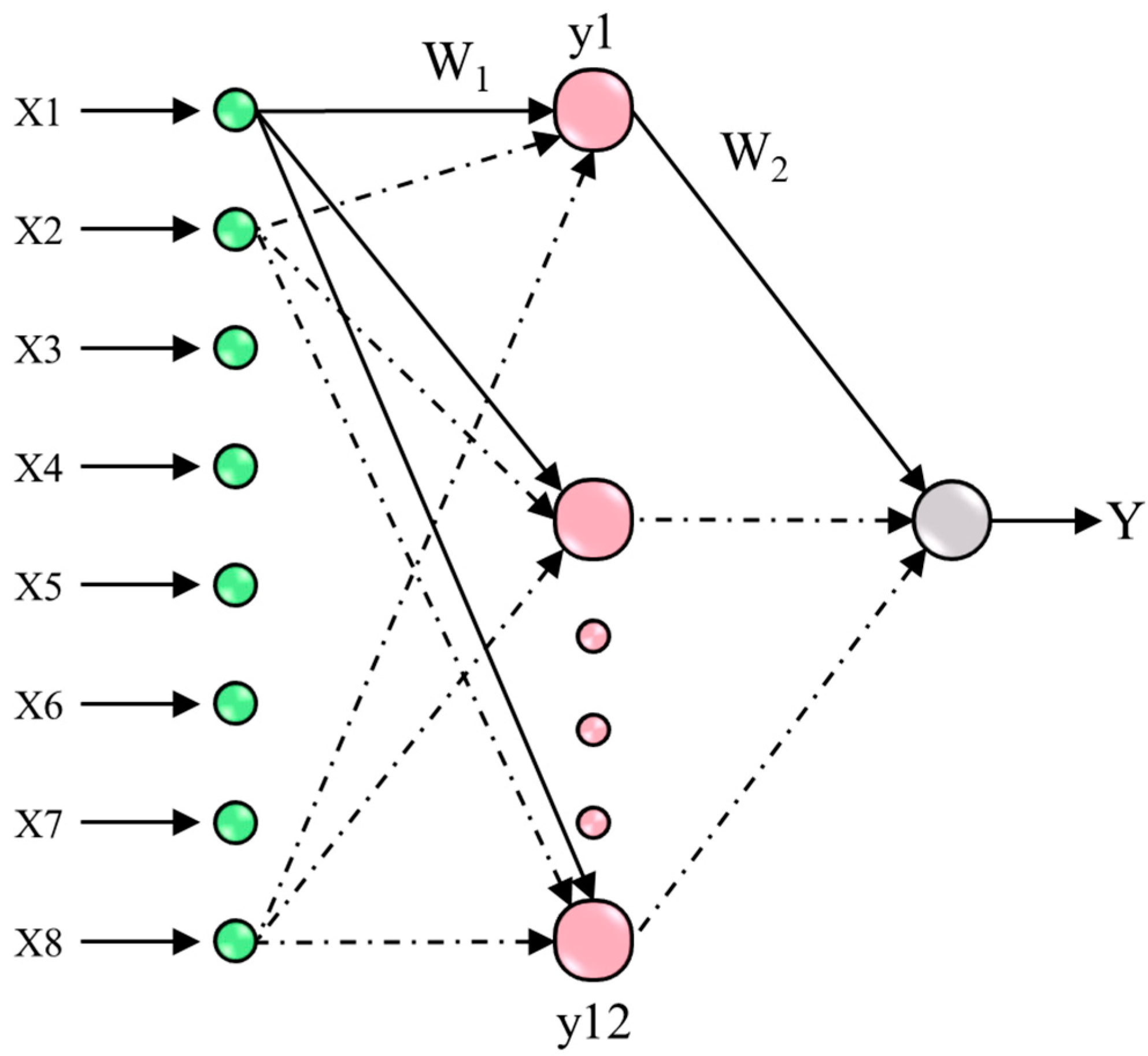
The architecture of the multilayer perceptron (MLP) neural network designed for this study is illustrated in Figure 1. The inputs to this MLP neural network encompass key agronomic traits of linseed, specifically, the number of days to emergence (x1), the number of days to flowering (x2), the number of days to maturity (x3), plant height (x4), the number of branches per plant (x5), the number of capsules per plant (x6), the number of seeds per capsule (x7), and the 1000-seed weight (x8). The output of the MLP network quantifies the seed yield per plant in grams (g).

The main objective is to build an MLP model (Y = MLP(x)) by precisely determining optimal weights (W1 and W2) [30]. These optimal weights are derived through the application of a neural network training algorithm, which includes a hidden layer. The determination of the number of neurons within this hidden layer (L2) is achieved through a process of trial and error, aiming to attain superior error performance on the training dataset. The weight update process for each weight is defined by the following equation (Equation (1)):

$$W\left(n+1\right)=W\left(n\right)-\eta \frac{\partial E}{\partial W}+\alpha \left(W\left(n\right)-W\left(n-1\right)\right)$$

(1)

where the variables n, E, η, and α represent the number of training iterations, the error, the learning rate, and the momentum factor, respectively.

To determine these optimal weights, a neural network training algorithm is employed, encompassing the following sequential steps [40]:

• Initialization: Initially, random values are assigned to the weights (W1 and W2).
• Forward Propagation: Input data, representing the agronomic traits of linseed, is propagated forward through the network. Neurons in each layer perform computations, ultimately producing an output.
• Error Calculation: The error, signifying the variance between the predicted output and the actual observed seed yield, is computed. This error quantifies the disparity between the model’s predictions and the ground truth.
• Backpropagation: Subsequently, the error is retroactively propagated through the network to update the weights. This process involves iteratively adjusting the weights to minimize the error between the predicted and actual values.
• Iteration: Steps 2 to 4 are iterated for a specified number of training iterations (n). During this phase, the network continually refines its weights to enhance predictive accuracy.

The Levenberg–Marquardt backpropagation algorithm was selected for use after meticulous consideration to optimize the neural network weights for predicting linseed seed yield and was underpinned by a series of carefully considered settings [41]. To ensure precise model performance, a stringent accuracy threshold of 0.001 was set for training termination. To safeguard against overfitting, a maximum of 10 validation failures was permitted, promoting robust generalization. Convergence during training was signified by a minimum performance gradient of 1 × 10⁻⁷. The initial damping factor (µ) was initialized at 0.001, strategically incorporated to expedite convergence and complemented by a µ decrease factor of 0.1, facilitating controlled weight refinement when needed. Moreover, when acceleration of convergence was required, a µ increase factor of 9 was invoked. The maximum value for µ was capped at 1 ×10⁻¹⁰, ensuring training stability. These settings collectively strike a harmonious balance between convergence speed and prediction precision, thereby establishing a robust foundation for linseed yield modeling employing MLP neural networks. The analysis in its entirety was conducted using a custom computer code developed within the MATLAB 9.5 software environment (MATLAB 2018b) (Figure S1). This bespoke code empowered the application of the MLP neural network model, configured with the specified settings, to predict linseed seed yield based on the pivotal agronomic traits under investigation.

2.3. Linseed Yield Modeling and Prediction Using MLR Methodology

In addition to the ANN methodology, the multiple linear regression (MLR) method is utilized in this study to model and predict linseed performance. This approach establishes mathematical relationships between linseed agronomic traits as independent variables and seed yield per plant as the dependent variable [42]. The independent variables are denoted as x1, x2, x3, x4, x5, x6, x7, and x8.

Within the context of MLR, an effort is made to formulate a linear equation that establishes a relationship between these agronomic traits and the linseed seed yield per plant (Y). The general form of the MLR model is expressed as follows:

$$\mathrm{Y}={\beta }_0+\sum _{i=1}^8{\beta }_i{x}_i+e_i$$

(2)

In this context, β₀ represents the intercept of the equation, while β₁ to β₈ denote the regression coefficients associated with each agronomic trait. These coefficients hold the key to determine the strength and direction of the relationship between each trait and seed yield. For the optimization of the regression coefficients (β values), the well-established statistical method known as ordinary least squares (OLS) is employed. OLS is used to minimize the sum of the squared differences between the predicted values (Y) based on the model and the actual observed seed yields [15].

In the MLR process, the assessment of the significance of regression coefficients (β values) is imperative. This assessment helps determine the statistical strength and relevance of each agronomic trait in predicting linseed seed yield, shedding light on which traits wield the most substantial impact on yield. To evaluate the significance of each β coefficient, we turn to statistical hypothesis testing, particularly utilizing the t-statistic. The t-statistic quantifies the ratio of the estimated coefficient to its standard error. The null hypothesis (H₀) proposes that the coefficient does not significantly differ from zero, suggesting that the corresponding independent variable exerts no effect on seed yield. Conversely, the alternative hypothesis (H₁) posits that the coefficient holds statistical significance, signifying a meaningful influence on seed yield. Additionally, the corresponding p-value is calculated for each t-statistic. This p-value measures the likelihood of obtaining a t-statistic as extreme as the one derived from our sample data, assuming the null hypothesis to be true. A low p-value, typically below 0.05, indicates compelling evidence against the null hypothesis, signifying the coefficient’s statistical significance.

Furthermore, an analysis of variance (ANOVA) table was constructed to evaluate the overall performance and significance of the MLR model. This table partitioned the total variability in seed yield into two components: one attributed to the linear regression model (explained variation) and the other stemming from random variability (unexplained variation).

To ascertain the contribution of each term in the model, the percentage of contributions is calculated using the following formula:

$$\mathrm{P}\mathrm{C}=\frac{{SS}_i}{{SS}_t}\times 100$$

(3)

Here, PC represents the percentage contribution associated with coefficient β_i. SS_i denotes the sum of squares of the term in the model, while SS_t represents the total sum of squares of the model. Furthermore, for the MLR analysis, the MATLAB 9.5 software was employed, with a particular emphasis on the fit linear regression model (fitlm) function, and Minitab was also utilized (Figure S2).

2.4. Performance Evaluation Metrics for MLP and MLR Models

In this study, both the MLP and MLR models underwent a thorough evaluation using three key criteria: the root mean squared error (RMSE), mean absolute percentage error (MAPE), and model efficiency (EF). The RMSE quantifies the average deviation between predicted and actual seed yield values, with lower values indicating a higher level of predictive accuracy. Meanwhile, MAPE offers insight into predictive performance by measuring the average percentage difference between predicted and actual values; a smaller MAPE signifies closer predictions to actual values. Lastly, EF assesses the model’s ability to capture data variance, with values closer to one indicating a robust predictive capability [43]. These criteria, when considered together, provided a comprehensive assessment of the models’ effectiveness in predicting linseed seed yield.

$$RMSE=\sqrt{\frac{1}{n}\sum _{i=1}^n{\left(Y_a-Y_p\right)}^2}$$

(4)

$$MAPE=\frac{1}{n}\sum _{i=1}^n\left|\frac{Y_a-Y_p}{Y_a}\right|$$

(5)

$$EF=1-\frac{\sum _{i=1}^n{\left(Y_a-Y_p\right)}^2}{\sum _{i=1}^n{\left(Y_a-\overline{Y_a}\right)}^2}$$

(6)

where Y_a and Y_p are actual and predicted seed yield, respectively. A superior model is characterized by RMSE and MAPE values closer to zero, and an EF value closer to one indicates its proficiency in predicting linseed seed yield.

2.5. Genetic-Algorithm-Based Optimization for Maximized Linseed Seed Yield

The primary objective of this undertaking is to ascertain the optimal configurations for agronomic variables that will yield the highest seed production within the specified range of model variables. The genetic algorithm procedure, which serves as the cornerstone of our study, is illustrated in Figure 2 [44,45]. In assessing performance and guiding the optimization process, the trained MLP neural network and the derived regression model were employed as our cost functions, with seed yield serving as the primary metric of interest. A unique approach was adopted, given that the genetic algorithm’s objective is cost minimization: a negative sign was introduced to the yield values, transforming our objective into a minimization task. Consequently, the various agronomic parameters became the focal point of our optimization efforts.

The pursuit of optimization commenced with the establishment of an initial population referred to as “chromosomes”, each containing a distinct combination of vital agronomic variables crucial for linseed cultivation. These variables encompassed key factors such as days to emergence, flowering, maturity, plant height, the number of branches, capsules per plant, seeds per capsule, and 1000-seed weight. Chromosomes were generated through a randomization process, representing a broad spectrum of agronomic conditions influencing linseed performance. Following the initial setup, each chromosome underwent a comprehensive evaluation. A predefined fitness function, either MLR or MLP, was employed to quantify the anticipated seed yield based on the unique agronomic variables within each chromosome. This served as the fundamental criterion for assessing their potential.

Advancing toward optimization involved implementing a selection mechanism that favored chromosomes with elevated fitness scores, signifying the likelihood of achieving superior expected seed yields. The chosen method for this purpose was tournament selection, ensuring that chromosomes exhibiting greater potential were more likely to serve as parents for the subsequent generation. The selected parent chromosomes were then paired to generate offspring through a crucial process known as crossover, involving the exchange of genetic information to mirror the inheritance of agronomic traits. The uniform crossover technique was employed, allowing for the creation of offspring with a wide array of trait combinations, thus enhancing the prospects of identifying optimal solutions. To maintain genetic diversity and prevent premature convergence toward suboptimal solutions, a mutation rate of 20% was introduced. This involved making random alterations to a portion of the genetic information in the offspring, toggling between 0 and 1, or vice versa. This mutation injected variability into the population, fostering the possibility of discovering more effective combinations of agronomic variables. The new generation was formed by combining the existing population with offspring from crossovers and mutants resulting from mutation. The selection mechanisms meticulously determined which individuals would continue into the next generation, ensuring a consistent population size. The genetic algorithm repeated these stages until a significantly superior solution was attained or a predetermined stopping criterion was met. Common stopping criteria included reaching a maximum number of generations or achieving a predefined level of seed yield optimization. This dynamic genetic algorithm optimization process played a pivotal role in identifying optimal solutions. The MATLAB code, featuring the MLP function, is showcased in Figure S3.

3. Result and Discussion

3.1. Results of Linseed Modeling Using Artificial Neural Networks

The decision to employ a single hidden layer in the MLP neural network, following Haykin’s (1998) recommendation, was based on the network’s proficiency in effectively approximating continuous functions [46]. This design choice aimed to strike a balance between complexity and performance. Through an extensive trial-and-error process, the network’s architecture was meticulously fine-tuned. Findings revealed that optimal performance was achieved when the hidden layer contained 15 neurons and the sigmoid activation function was employed. This specific configuration enabled the network to adeptly capture and model the intricate relationships among the eight independent variables and linseed yield.

To rigorously assess the performance of the MLP model, our extensive dataset, consisting of 300 field data points, was systematically divided into three distinct subsets. These subsets were carefully stratified to ensure representative samples: the training dataset, comprising 240 data points; the validation dataset, containing 30 data points; and the test dataset, consisting of the remaining 30 data points. Such meticulous data partitioning was essential to validate the robustness and generalization capability of the model.

A visual representation of the MLP model’s convergence during the training phase is presented in Figure 3. The figure tracks the evolution of mean squared error (MSE) for each training, validation, and test dataset over multiple iterations. Our analysis of MSE dynamics throughout the training process yielded valuable insights. Notably, the MLP network demonstrated rapid learning capabilities, effectively capturing the nuances of linseed yield changes in response to the eight independent variables. Impressively, this learning plateaued by the end of the fifth iteration epoch. Subsequent iterations, beyond this point, did not significantly enhance the model’s performance on the validation dataset, as indicated by a noticeable increase in error. Consequently, the MSE for the training and testing datasets remained relatively stable, underscoring the proficiency of the MLP model in predicting linseed yield. The fifth iteration epoch yielded an outstanding mean square error value of 0.0015, highlighting the model’s robust performance.

The outcomes of the comprehensive analysis of the perceptron neural network model are meticulously presented in

Table 2. Evaluation criteria for the neural network model of linseed yield prediction.

	Train	Validation	Test	Total
RMSE (g/plant)	0.064	0.040	0.065	0.062
MAPE (%)	3.599	2.684	4.377	3.585
EF (%)	0.978	0.989	0.972	0.979

. The table showcases error criteria, including MAPE, RMSE, and EF metrics, for each of the training, validation, and testing datasets, and the combined dataset. It is observed that the highest RMSE and MAPE values were 0.065 t/ha and 4.5%, respectively. These values underscore the exceptional performance of our trained neural network model. The lower RMSE and MAPE values are particularly noteworthy, indicating a remarkably close alignment between our model’s predicted trends and the actual observed values. This suggests that our MLP neural network model has effectively captured the underlying patterns and relationships within the data. Notably, the EF metric consistently exceeded 0.97 across all datasets. These high EF values reaffirm the robustness and accuracy of our model in predicting linseed yield based on agronomic traits. It is worth highlighting that the test dataset, representing novel data for our MLP neural network, exhibited slightly higher MAPE and RMSE values compared to the other datasets. However, these values remained well within the acceptable range for error metrics. Furthermore, the EF score for the test set remained impressively high, surpassing the 0.97 threshold. These results collectively emphasize the predictive power and reliability of our MLP neural network model, even when confronted with previously unseen data.

The performance assessment of the MLP neural network model for predicting linseed yield involved a meticulous comparison of the observed and modeled yield, with a focus on mean and variance metrics (

Table 3. Statistical properties and comparison of actual and predicted data.

	Train Phase		Validation Phase		Test Phase
	Mean	Variance	Mean	Variance	Mean	Variance
Desired value	1.332	0.188	1.296	0.169	1.271	0.154
Prediction value	1.334	0.181	1.293	0.163	1.277	0.150
p-value	0.947	0.770	0.976	0.926	0.949	0.929

). The results reveal a remarkable concordance between the mean and variance values of both datasets—observed and modeled—across the training, validation, and test phases. Importantly, statistical analysis showed that there existed no statistically significant difference between these datasets, with a p-value exceeding 0.9, indicating a strong alignment between the predicted and actual yield values. This congruence underscores the proficiency of the MLP neural network in accurately capturing the linseed yield patterns and reflects its effectiveness in modeling this complex agronomic system.

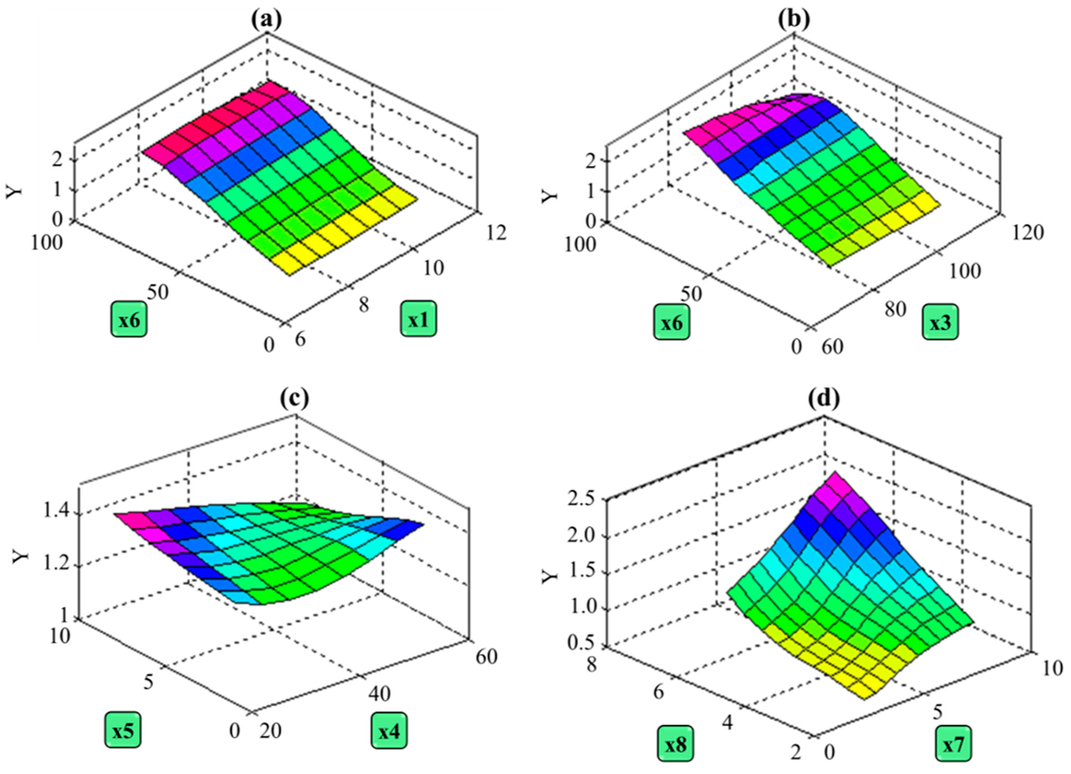
Based on the results obtained from the test phase of the MLP neural network, as presented in Table 2 and Table 3, it is clear that the MLP model demonstrates exceptional generalization capability, establishing it as a dependable tool for predicting linseed yield. Using the final MLP model, a three-dimensional graph was created to illustrate the relationship between the dependent variable (linseed yield) and two independent variables while holding the others at their mean values. For instance, in Figure 4, specific relationships between variables are depicted. This graph demonstrates how changes in independent variables relate to variations in seed yield.

Referring to the findings in

Table 4. Analysis of regression model variance in the prediction of linseed yield by independent agronomic variables.

Term	DF	SS	p-Value	Term	DF	SS	p-Value
x1	1	5.48	0.15	x5	1	8.11	0.19
x2	1	0.08	0.09	x6	1	16.72	0.00
x3	1	4.00	0.03	x7	1	7.66	0.00
x4	1	2.99	0.04	x8	1	5.81	0.00
Error	291	3.61	R2 = 93.37%, R2adj = 93.19%

, it is revealed in Figure 4a that alterations in the number of days to emergence (x1) did not significantly impact seed yield. Conversely, the range of variation in seed yield was more pronounced when adjusting the number of days to maturity (x3) and the number of capsules per plant (x6), spanning from 0 to 2.5. However, for plant height (x4) and the number of branches per plant (x5) (Figure 4b,c), this range was narrower, ranging from 1 to 1.4. These results suggest that the number of days to maturity and the number of capsules per plant exert a more substantial influence on seed yield compared to plant height and the number of branches per plant. As a result, the linseed breeding program can focus on developing high-yielding varieties with suitable plant heights that facilitate mechanized harvesting. This observation aligns with the findings of Sankari (2000), which reported no significant relationship between seed yield and plant height [47]. Additionally, Soto-Cerda et al. (2014) emphasized the positive correlation between grain yield and its components in linseed, albeit a negative association with days to flowering, the number of branches per plant, and plant height [48].

The results also highlight that an increase in the number of seeds per capsule (x7) and 1000-seed weight (x8) leads to improved linseed performance. Notably, the impact of an increase in the number of seeds per capsule (x7) was more pronounced at higher levels of this variable. This observation underscores the significance of the number of seeds per capsule and 1000-seed weight in relation to grain yield [48,49]. The number of capsules per plant (x6) was also found to significantly influence grain yield [49], suggesting that enhancements in these traits could indirectly boost seed yield. Conversely, the associations between the number of seeds per capsule and 1000-seed weight were relatively weak in several studies [4,11,50], and only a slight but significant relationship was identified between the number of capsules per plant (x6) and the number of seeds per capsule and 1000-seed weight in linseed [11,50].

These findings collectively contribute to a deeper understanding of the intricate relationships governing linseed yield and its underlying agronomic factors, paving the way for more targeted breeding and cultivation strategies.

3.2. Results of Linseed Modeling Using Multiple Linear Regression Model

The results of the analysis of variance for the multiple linear regression model used to predict linseed performance are presented in Table 4. The p-values associated with the independent variables reveal significant effects on seed yield. Specifically, three variables—namely, the number of capsules per plant (x6), the number of seeds per capsule (x7), and 1000-seed weight (x8)—exhibited a substantial impact on seed yield at a highly significant level, with p-values less than 0.01. Additionally, the number of days to maturity (x3) and plant height (x4) showed significant effects at a 5% probability level, while the number of days to emergence (x1), the number of days to flowering (x2), and the number of branches per plant (x5) were not found to be significant predictors.

The coefficient of determination (R²) and the adjusted coefficient of determination (R²adj) were calculated to assess the model’s effectiveness in explaining the variation in seed yield. These metrics indicate that the fitted regression model can account for approximately 94% of the variance observed in seed yield. Similar studies, such as Dyjas et al. (2005) [51], also developed regression models to estimate seed yield, achieving an R² value of 68% by considering traits such as plant density, the number of capsules per plant, the number of seeds per capsule, and 1000-seed weight. Abbas (2013) supported these findings, emphasizing the significant partial coefficient of determination attributed to factors like fiber percentage, 1000-seed weight, the number of seeds per capsule, and technical length per plant in explaining the total variation in linseed yield per plant [52]. These results underscore the importance of specific agronomic traits in predicting linseed yield.

The contribution percentages for each agronomic variable to linseed seed yield are visually presented in Figure 5. Amongst the considered agronomic variables, the number of capsules per plant (x6) emerged as the most influential factor, contributing significantly with a substantial impact of 30.7%. In contrast, the number of days to flowering (x2) exhibited the lowest contribution, accounting for a mere 0.2% of the variance in seed yield. Additionally, four other agronomic variables, namely the number of days to emergence (x1), the number of branches per plant (x5), the number of seeds per capsule (x7), and 1000-seed weight (x8), displayed varying levels of contribution, falling within the range of 10 to 15%. These findings illuminate the varying degrees of influence that these agronomic traits have on linseed yield, underscoring the significance of individual variables within the predictive model.

In addition to the previously presented results, correlation analyses were conducted to investigate the relationship between the independent variables and the dependent variable. The findings indicate that, excluding the number of days to flowering (x2), a significant correlation at the 1% significance level was observed between the dependent variable, representing the seed yield per plant in grams, and all other independent variables or agronomic factors. These correlation values are consistent with the contribution percentages obtained for each agronomic variable, further substantiating their significance. Specifically, correlation values of −0.42, −0.07, 0.17, −0.28, 0.40, 0.58, 0.41, and 0.43 were identified for the number of days to emergence (x1), the number of days to flowering (x2), the number of days to maturity (x3), plant height (x4), number of branches per plant (x5), number of capsules per plant (x6), number of seeds per capsule (x7), and 1000-seed weight (x8), respectively, in relation to the seed yield per plant. These correlation results provide additional insights into the nature of the relationship between each independent variable and the seed yield per plant in grams.

Equation (7) presents the regression model that predicts linseed yield based on independent agronomic variables:

$$Y=-1.983-0.011 x_1+0.0039 x_2-0.0036 x_3-0.0028 x_4+0.0112 x_5+0.0259 x_6+0.192 x_7+0.261 x_8$$

(7)

3.3. Comparing the Estimation Abilities of the MLR and ANN in Predicting Linseed Yield

The adequacy of the regression model was thoroughly assessed by examining two critical diagnostic plots, as depicted in Figure 6: the normal probability plot of residuals and the residuals vs. fitted plot. In Figure 6a, the normal probability plot displays the standardized errors derived from the regression model. This plot demonstrates that the residuals tend to follow a relatively normal distribution, aligning with one of the fundamental assumptions of linear regression. However, it is worth noting that some residuals deviate significantly from the normal line, suggesting the potential presence of outliers or influential data points. Figure 6b delves into assessing the constant variance assumption, a crucial element in linear regression modeling. This plot reveals that the variance of error terms remains relatively consistent across the range of predicted values. The roughly uniform spread of residuals indicates that the model’s performance is consistent throughout the data range. Considering the insights gleaned from Figure 6, it is evident that the extracted regression model demonstrates a reasonable level of reliability. However, acknowledging the presence of potential outliers or influential observations, as indicated by the deviations from normality observed in Figure 6a, is imperative. Additionally, while the variance of error terms appears relatively stable, further investigations, such as the identification of influential data points, might be necessary to refine the model and enhance its reliability in capturing variations in linseed yield.

Assessing the performance of the regression model involves a comprehensive examination of various metrics, including RMSE, MAPE, EF, and a statistical comparison between the actual and predicted data.

Table 5. Evaluation criteria of the fitted regression model.

p-Value		Criteria Error
Mean	Variance	RMSE (g/Plant)	MAPE (%)	EF (%)
1.000	0.553	0.109	6.793	93.37

provides a detailed overview of these key metrics for the fitted regression model (Equation (7)). Comparing the mean and variance of real data with those predicted by the model is crucial for evaluating the model’s validity. The p-values presented in Table 5 confirm that there is no significant difference between the mean and variance of the real data and the predicted data obtained from Equation (7) at the 1% significance level.

Interpreting the values of the error indices and considering the p-values, we can conclude that the regression model demonstrates a commendable ability to predict linseed yield. The RMSE and MAPE of the MLP model were notably lower, approximately 43% and 17%, respectively, compared to the RMSE and MAPE of the MLR model. Additionally, the EF of the MLR model lagged behind the MLP model by nearly 5%. These findings suggest that the MLP model outperformed the MLR model in terms of predictive accuracy, emphasizing its potential as an effective tool for linseed yield prediction.

For a more comprehensive assessment of the performance of the trained MLP neural network and the fitted regression model, Figure 7 provides a frequency histogram of the errors associated with each model. Understanding the distribution of errors is crucial for assessing the predictive capabilities of these models. The variation in errors spans from −0.25 to 0.29 in the MLP model, highlighting the model’s ability to make predictions within a relatively narrow margin. In contrast, the MLR model exhibits a wider range of error variation, ranging from −0.56 to 0.5. When examining the error distribution within a smaller range, specifically between −0.05 and 0.05, it is evident that a substantial proportion of errors from both models falls within this interval. Approximately 70% of the errors from the MLP model and 55% from the MLR model are concentrated within this range. This indicates that both models are proficient at making predictions that closely align with the actual values, with the MLP model displaying a slightly higher percentage of predictions falling within this desirable range. These findings provide valuable insights into the accuracy and reliability of both models in predicting linseed yield, with the MLP model demonstrating a marginal advantage in terms of error distribution.

In pursuit of a robust evaluation of the models’ performance, it is essential to examine the agreement between real and predicted data, a fundamental aspect of model validation. As depicted in Figure 8, a comparison is made between actual data and the predictions generated by the MLP and MLR models. A reliable model is characterized by a regression line that exhibits a slope close to one and an intercept near zero, ultimately yielding an R² value approaching one. Such characteristics signify that the model’s predictions closely align with the actual data, indicating its proficiency in capturing the underlying patterns and trends. Upon closer examination, it is evident that the MLP model outperforms the MLR model in terms of its agreement with real linseed yield data. The slope of the regression line for the MLP model is notably closer to one when compared to the MLR model, and its intercept is significantly closer to zero. This is further corroborated by the R² value, which is approximately 6.4% higher for the MLP model in comparison to the MLR model. These findings underline the superior ability of the MLP model to predict linseed yield while maintaining a stronger alignment with actual data, further substantiating its reliability and accuracy.

To evaluate the generalizability of the MLP neural network model, additional experiments were conducted, modifying the size of the training dataset from 80% to 50%, and adjusting the sizes of the validation and testing datasets accordingly. The results of this investigation are presented in

Table 6. The results of evaluating the generalizability of MLP neural network performance across diverse conditions.

Train/Validation/Test (%)	Criteria	Train	Validation	Test	Total
80/10/10	RMSE (g/plant)	0.064	0.040	0.065	0.062
	MAPE (%)	3.599	2.684	4.377	3.585
	EF (%)	0.978	0.989	0.972	0.979
70/15/15	RMSE (g/plant)	0.054	0.046	0.072	0.055
	MAPE (%)	3.211	2.754	4.875	3.392
	EF (%)	0.989	0.968	0.952	0.980
60/20/20	RMSE (g/plant)	0.041	0.065	0.098	0.057
	MAPE (%)	2.834	2.950	6.786	3.647
	EF (%)	0.999	0.950	0.932	0.975
50/25/25	RMSE (g/plant)	0.070	0.093	0.112	0.086
	MAPE (%)	3.925	3.450	8.437	4.930
	EF (%)	0.902	0.905	0.901	0.903

. The findings indicate that, with a reduction in the size of the training set to 60%, improved prediction performance is observed during the training phase. This enhancement can be attributed to a decrease in the variability in changes in the response variable pattern, enabling the network to better capture underlying relationships. However, as the training set size further decreases, the performance during the training phase deteriorates, likely due to insufficient patterns to adequately train the model. Furthermore, the reduction in the size of the training set consistently weakens prediction performance in the test and validation phases. This behavior is attributed to the inherent limitation of the model arising from the insufficient availability of patterns for training. Despite this, prediction errors for training set sizes up to 60% remain within acceptable ranges, demonstrating promising results when compared to the MLR model (Table 6). In conclusion, based on the findings, it can be confidently stated that the generalizability of the MLP model is acceptable for training set sizes up to 60% and its predictions can be deemed reliable. These results underscore the potential and effectiveness of the MLP neural network in our research context.

Recognizing the remarkable capabilities demonstrated by the MLP neural network in this research, it is imperative to acknowledge its inherent limitations. These limitations encompass the tendency of MLP models to overfit, particularly when confronted with intricate datasets or limited training data. The intricate architecture and numerous hidden layers often contribute to the lack of interpretability in MLP models, designating them as ‘black boxes’. Moreover, MLP models exhibit high sensitivity to hyperparameters, demanding meticulous tuning. Inadequate data may lead to either underfitting or overfitting. Additionally, the computational demands of MLP models can present challenges in real-time or resource-constrained applications. Therefore, a comprehensive consideration of all aspects and exercising caution is essential when employing MLP models.

3.4. Optimization of Linseed Yield Using Genetic Algorithm

The genetic algorithm (GA) was employed to determine the optimal combinations of agronomic variables, with the objective of maximizing linseed yield within the allowable range for each variable after completing and evaluating the neural network and regression models. The convergence trajectory of the GA, optimized using two cost functions, MLP and MLR, is thoughtfully illustrated in Figure 9. Notably, convergence was achieved after approximately 170 and 220 generations of solutions, respectively, when utilizing MLP and MLR as cost functions. Intriguingly, due to the inherent linearity, the MLR model exhibited a quicker convergence rate compared to the MLP model. The initial generation of solutions derived through MLP closely approximated the final generation of optimized solutions generated by MLR. This observation provides valuable insight into the optimization process, highlighting the convergence dynamics and suggesting the adaptability of the GA to varying cost functions.

The results of the optimization process, aimed at improving linseed yield using the genetic algorithm, with both the MLP neural network and the regression model as cost functions, are meticulously documented in

Table 7. Optimal agronomic parameters * for maximizing linseed seed yield.

Model	x1 (Days)	x2 (Days)	x3 (Days)	x4 (cm)	x5	x6	x7	x8 (g)	Maximum Yield (g/Plant)
MLP	9.15	47.35	80.75	35.26	1.90	85.67	8.50	6.61	4.40
MLR	7.00	72.00	75.00	23.00	9.50	85.67	8.50	6.61	3.57

* The agronomic traits used as independent variables include number of days to emergence (x1), number of days to flowering (x2), number of days to maturity (x3), plant height (x4), number of branches per plant (x5), number of capsules per plant (x6), number of seeds per capsule (x7), and 1000-seed weight (x8).

. Remarkably, the maximum seed yield calculated for the MLP and MLR models exceeded the upper limits of the observed yield range. This disparity can be attributed to the inherent characteristics of these models. Notably, when guided by the MLP model, the GA yielded a remarkable 19% increase in maximum yield compared to the MLR-guided optimization. This difference underscores the superior capacity of the MLP model to capture the nonlinear yield dynamics; a direct contrast to the linear nature of the MLR model.

Interestingly, optimal levels for the number of capsules per plant (x6), number of seeds per capsule (x7), and 1000-seed weight (x8) were remarkably similar for both the MLP and MLR models. This consistency highlights the pivotal role these variables play in achieving maximum yield. However, intriguing disparities emerge when considering the optimal values for other variables. For instance, while the MLR model favored the lowest value of the number of branches per plant (x5) for maximum seed yield, the MLP model diverged from this pattern. These optimization results hold significance for plant breeding experts aiming to enhance crop yield, a critical breeding objective.

Crop yield, being a multifaceted trait, is shaped by a myriad of contributing factors with complex interactions. Often, altering one component may be counterbalanced by changes in another. Our findings, in conjunction with prior research, highlight the paramount importance of three agronomic traits, the number of capsules per plant, the number of seeds per capsule, and 1000-seed weight, in influencing linseed yield. For both models, these traits’ optimal values were calculated at approximately 85.67 (capsules), 8.50 (seeds per capsule), and 6.61 (g), respectively. However, breeders should consider the optimal values for other variables as well.

For the MLP model, optimizing linseed yield involved striving for an early flowering date, a later maturity date, and greater plant height, with the respective optimal values being approximately 47 days, 81 days, and 35 cm. In contrast, the MLR model suggested different optimal values, around 72 days, 75 days, and 23 cm, for the same variables. This divergence underscores the flexibility of our approach, allowing breeders to tailor their optimization strategy based on specific objectives.

Furthermore, insights into trait heritability provide a valuable guide for breeders. Traits with high heritability, such as plant height, days to flowering, and maturity, offer relatively straightforward avenues for improvement. In contrast, traits with lower heritability, like the number of branches per plant, present more significant challenges in achieving substantial gains through selection alone. Thus, to enhance linseed yield efficiently, breeders can focus on optimizing traits with higher heritability, requiring minimal manipulation of those with lower heritability. This knowledge can be a cornerstone for informed breeding strategies, ultimately leading to improved linseed varieties and increased yield.

4. Conclusions

This study conducted a thorough assessment of the predictive capabilities of two distinct models: multiple linear regression (MLR) and multilayer perceptron artificial neural network (MLP) for estimating linseed seed yield. Modeling efforts were based on a comprehensive dataset that included key agronomic variables, such as the number of days to emergence (x1), number of days to flowering (x2), number of days to maturity (x3), plant height (x4), number of branches per plant (x5), number of capsules per plant (x6), number of seeds per capsule (x7), and 1000-seed weight (x8). This dataset spanned two years of field data collected from the Research Farm at Valieasr University of Rafsanjan, Iran. Additionally, a genetic algorithm (GA) was employed to determine optimal conditions for maximizing linseed seed yield. The salient findings of this research can be summarized as follows:

-

The MLP model consistently demonstrated remarkable performance in accurately predicting linseed seed yield across training, validation, and test phases, further establishing its reliability as a predictive tool.

-

ANOVA results emphasized the significance of most independent variables at the 1% or 5% significance levels, with exceptions being the number of days to emergence (x1), number of days to flowering (x2), and number of branches per plant (x5).

-

Evaluation of the adequacy of the fitted regression models affirmed the relative reliability of the MLR model.

-

Direct comparison of the MLP and MLR models revealed MLP as the preferred choice due to its lower RMSE and MAPE values, along with its higher R² and EF values.

-

The GA played a pivotal role in determining optimal agronomic parameter values for maximizing linseed seed yield. Interestingly, the optimization outcomes varied when employing two different cost functions, namely the MLP and MLR models.

-

Our study advocates for the adoption of neural network models, such as MLP, for precise yield predictions not only in linseed cultivation but also across diverse crops, relying on key agronomic parameters. Also, the application of GAs is invaluable for addressing optimization challenges within the realm of biotechnology, particularly in the context of genetic modification.

In conclusion, this research combined data-driven modeling and optimization techniques to enhance our understanding of linseed seed yield prediction. These findings have broader implications for agricultural practices and biotechnological advancements, emphasizing the pivotal role of advanced modeling and optimization methodologies in crop yield optimization and genetic modification processes.