Quantitative Analysis of Vertical and Temporal Variations in the Chlorophyll Content of Winter Wheat Leaves via Proximal Multispectral Remote Sensing and Deep Transfer Learning

Abstract

Quantifying the vertical distribution of leaf chlorophyll content (LCC) is integral for a comprehensive understanding of the physiological status and function of winter wheat crops, having significant implications for crop management and yield optimization. In this study, we investigated the vertical LCC trait of winter wheat during two consecutive field growth seasons using proximal multispectral imaging measurements to evaluate vertical variations of LCC within winter wheat canopies. The results revealed the non-uniform vertical LCC distribution varied across the entire growth season. The effects of nitrogen fertilization rate on LCC among vertical layers increased gradually from upper to lower layers of canopy. To enhance LCC prediction accuracy, this study proposes a deep transfer learning network model for leaf trait estimation (LeafTNet). It integrates the advantages of physical radiative transfer simulations with deep neural network through transfer learning. The results demonstrate that the LeafTNet achieved remarkable predictive performance and strong robustness. Furthermore, the proposed method exhibits superior estimation accuracy compared to empirical statistical method and traditional machine learning method. This study highlights the performance of LeafTNet in accurately and efficiently quantifying LCC from proximal multispectral data, which provide technical support for the estimation of the vertical distribution of leaf traits and improve crop management.

1. Introduction

Accurate and timely monitoring of crop growth status is pivotal for estimating crop yield and advancing agricultural sustainability [1]. The efficient management of winter wheat cultivation requires a comprehensive understanding of various physiological parameters. Among these parameters, leaf chlorophyll content (LCC) emerges as a vital indicator of photosynthetic activity and plant vigor. Moreover, LCC plays a crucial role in assessing nutrient deficiencies, environmental stress, or pathogen attacks, allowing for the early detection and diagnosis of potential issues affecting crop health [2,3,4,5]. Understanding vertical and temporal variations in chlorophyll content distribution within the crop canopy can provide valuable insights into the dynamic changes in crop growth status, helping optimize agronomic practices for enhanced crop breeding and management [6,7].

During plant growth and development, as the canopy structure undergoes continuous changes, the biochemical parameters of plants exhibit non-uniform vertical distribution within the crop canopy [8,9]. The reasons for this heterogeneity may involve the combined effects of multiple factors. The variability in light radiation in the vertical direction within the canopy has been identified as a major driving factor [10,11]. Upper leaves, exposed to more sunlight, receive stronger photosynthetic stimulation, thereby promoting chlorophyll synthesis. In contrast, lower leaves, hindered by upper leaves, exhibit lower photosynthetic efficiency, resulting in lower chlorophyll content. In terms of nutritional factors, nitrogen, as a readily transportable nutrient, enhances photosynthesis efficiency through its redistribution in plants, and different nitrogen application levels also affect non-uniform distribution [12,13]. Additionally, differences in growth stages also play a role in vertical heterogeneity. Senescent leaves may gradually lose chlorophyll, while newly grown leaves demonstrate higher chlorophyll synthesis activity, leading to relatively higher chlorophyll content in upper new leaves. These factors may affect chlorophyll synthesis and distribution by influencing plant metabolism and physiological activities.

Advancements in remote sensing technologies have opened new avenues for the accurate monitoring of crop vertical distribution characteristics. According to observation approaches, existing studies can be divided into two types: multi-angle observations and top-view observations with the non-imaging spectroradiometer [8]. Kong et al. conducted multi-angle observations on wheat canopy using a non-imaging spectroradiometer, revealing that angles near the hotspot were more suitable for estimating upper canopy chlorophyll, while smaller angles from the nadir were more accurate in assessing chlorophyll in the lower canopy [14]. Wu et al. explored the vertical heterogeneity of chlorophyll in wheat canopies, utilizing canopy reflectance data from multi-angle observations to determine leaf chlorophyll content in different vertical layers [15]. He et al. [9] and Duan et al. [16] explored the relationship between different vegetation indices and vertical nitrogen distribution within the rice and wheat canopy, respectively, and both studies were conducted based on the canopy reflectance data from top-view observations using a non-imaging spectroradiometer. Wang et al. [17] suggested that combining top-view observation and hyperspectral data can enhance the accuracy of estimating the bottom layer in the fraction of intercepted photosynthetically active radiation. Li et al. [18] investigated variations in crop traits among different leaf layers and modules (including leaves, stems, and spikes) within wheat canopies, and the impact of these layers and modules on non-imaging canopy spectral characteristics through top-view observations. However, whether they are multi-angle or top-view observations with the non-imaging sensing for the LCC vertical inversion, these approaches cannot avoid the obscuration of lower leaves by upper leaves in the canopy, overly emphasizing the contribution of upper leaves to spectral components, and thus may not comprehensively describe the vertical heterogeneity within the crop canopy. Moreover, these approaches are also unable to accurately depict the LCC variation at leaf-scale because of the position mismatching between sampling analysis and spectral measurement based on five-point sampling using the non-imaging spectrometer [19]. The use of multispectral proximal imaging allows for a more detailed, accurate, and lower-cost evaluation of LCC at a fine scale, enabling researchers to capture subtle variations over different leaf layers.

Despite the surging interest in the role of chlorophyll status in crops, most studies have been conducted on the spectra–trait relationship for sunlit leaves at the upper layer within the canopy, the vertical variability of chlorophyll has been neglected in studies using canopy spectral reflectance measured by satellites or drone-based remote sensing [20,21,22,23]. In these studies, the entire canopy was considered as a homogenous plane, which limits robustness of canopy remote sensing and reduces it the practical value. The possible reasons for the limited or lack of studies thereof are the insufficient and complex collection of field measurements data at different leaf layers within the canopies [20] and the lack of effective observation methods based on remote sensing to characterize the vertical heterogeneity in leaf traits and spectra. Extensive evidence suggests that chlorophyll content in flag leaves at the jointing and filling stages and three upper layer leaves at the booting and anthesis stages are commonly used to assess canopy chlorophyll status [16,23], whereas other studies indicated that middle layer leaves at anthesis stage are more suitable as indicators for canopy chlorophyll diagnosis [24,25]. There is controversy over the effective leaf layers that represent canopy chlorophyll status during various growth stages. In addition, some reports indicated that nitrogen fertilization application in wheat plants influenced vertical LCC distribution, as crops respond to nitrogen stress by altering chlorophyll content in different vertical leaf layers to maintain photosynthetic efficiency [10,26]. However, to date, few studies have conducted sufficient multi-temporal observations to analyze the characteristics of vertical LCC distribution in winter wheat under different nitrogen treatments in a systematic manner and construct a quantitative model to reveal the intrinsic mechanism between LCC and leaf spectral imaging reflectance at a fine scale.

This study focuses on quantifying the vertical LCC distribution of winter wheat under various nitrogen treatments from multispectral proximal imaging data at different growth stages. The specific objectives of this study are to (i) explore the characteristic of vertical LCC distribution within winter wheat canopies and temporal variations in LCC vertical profiles across the growth season, (ii) determine the effective leaf layers indicating the canopy LCC status in winter wheat, (iii) construct an effective and universal deep transfer learning model by leveraging transfer knowledge from physical radiative transfer simulations for accurate quantitative monitoring LCC.

2. Materials and Methods

2.1. Field Experimental Site

The experiments were conducted in 2023 and 2024 at the experimental station of the Jiangsu Xuhuai Regional Institute of Agricultural Science (33°16′58″ N, 117°17′23″ E), located in Xuzhou, Jiangsu Province, China. The climate here is characterized as temperate semi humid monsoon climate, with an annual average temperature of 14.5 °C, annual average rainfall of 727.6 mm, and frost-free period of 200–220 days. The predominant soil type is yellow brown soil. Winter wheat is commonly sown in mid-October and harvested in early June of the next year.

Two and three winter wheat varieties were cultivated with different N fertilization treatments in 2022–2023 and 2023–2024, respectively (

Table 1. Basic information of field experiments of winter wheat.

Year	Variety	N Rate (kg/ha)	Date	Growth Stage Description
2022–2023	XM28, XM35 (Medium Gluten Wheat)	0	9 April	Booting Stage
		180	19 April	Heading Stage
		225	27 April	Anthesis Stage
			13 May	Milk Stage
			20 May	Dough Stage
2023–2024	XM35 (Medium Gluten Wheat) XM44, XM49 (Strong Gluten Wheat)	225	12 April	Heading Stage
		270	24 April	Anthesis Stage
			2 May	Early Milk Stage
			10 May	Late Milk Stage
			20 May	Dough Stage

). The wheat field adopted a split-plot design. Each variety was cultivated in a plot with an area of 7.5 × 10 m². The nitrogen fertilizer was applied in two splits, comprising both base and topdressing fertilizer applications in a 1:1 ratio. The nitrogen fertilizer was applied before sowing and at the jointing state. More information on the field management can be found in the study of [23]. Irrigation application followed natural rainfed conditions, and herbicide application employed local standard practices in winter wheat production. The sample collections and field measurements were conducted at five stages during each wheat growth season. A total of 324 and 335 leaf samples were collected during the 2022–2023 and 2023–2024 growth seasons, respectively. The experimental details are shown in Table 1.

2.2. Field Data Acquisition and Preprocessing

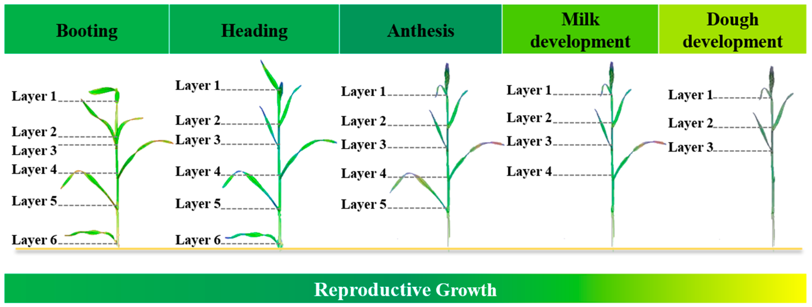
2.2.1. Leaf Sampling and Image Collection

The chlorophyll variables at the different leaf layers were measured using field sampling and subsequent laboratory analysis. At each growth stage, three wheat plants were sampled randomly for each treatment, and each leaf of the sampled plants was measured to determine the chlorophyll content. Leaves were collected from different vertical layers, denoted as layer one (L1), two (L2), three (L3), four (L4), five (L5) and six (L6), spanning from the top to the bottom of the canopy (Figure 1). The height of each leaf layer was measured synchronously, representing the distance from the position of the leaf collar to the ground.

The leaf spectrum images were measured using a DJI Phantom 4 with the P4 Multispectral Camera (DJI Technology Company Ltd., Shenzhen, China). The equipment integrates a visible-light CMOS sensor and five optical filter sensors with different center wavelengths and spectral resolutions of 450@16 nm, 560@16 nm, 650@16 nm, 730@16 nm and 840@26 nm. Measurements were conducted during sunny days between 10:00 and 14:00 local time.

The sample leaves were positioned on a black background board, with calibration labels affixed for subsequent band registration during data preprocessing. The tip, middle, and root positions of each leaf blade were fixed on the board using narrow black double-sided tape. The images of the leaves were acquired at a height of 1.5 m with top-view observation. Throughout the acquisition process, a white calibration panel was deployed on the ground for reflectance calibration.

2.2.2. Chlorophyll Measurement

After the leaf reflectance measurements, the collected leaf samples were labeled and subsequently enclosed in an insulator before being dispatched to the laboratory for biochemical analysis. The chlorophyll concentrations (Chl_a+b, unit: mg/L) were determined utilizing the wet lab extraction technique [27]. For laboratory analysis, fresh leaves were clipped using a leaf borer to facilitate the calculation of the leaf disk area and mass. The absorbance of the extracted substances was measured at 665 nm and 649 nm using a UV–VIS spectrophotometer (MAPADA UV-1800PC, Shanghai, China). The leaf chlorophyll content (LCC) was determined as follows:

$$LCC({\text{µ}\mathrm{g}/\mathrm{cm}}^2)={\displaystyle \frac{Ch{l}_{a+b}(\mathrm{mg}/\mathrm{L})\times V(\mathrm{mL})\times n}{{\mathrm{disc}\mathrm{area}(\mathrm{cm}}^2)}},$$

(1)

where Chl_a+b represents chlorophyll concentration. V and n represent the volume and volume concentration of the extract solution, respectively.

The LCC_total refers to the total chlorophyll content of the entire canopy. It is determined as the total chlorophyll accumulation per unit of leaf area. The leaf area corresponding to the leaf layer was determined through manual measurements of the maximum length and width of the individual leaves [28]:

$$Leafarea{(\mathrm{cm}}^2)=\mathrm{length}\times \mathrm{width}\times 0.65,$$

(2)

$$LC{C}_{t\mathrm{o}tal}={\displaystyle \frac{{\displaystyle \sum _{i=1}^m(LC{C}_{Li}\times LeafAre{a}_{Li})}}{TotalArea}},$$

(3)

where m denotes the number of leaf layers in the canopy, LCC_Li and Leaf Area_Li refer to the leaf chlorophyll content (μg/cm²) and leaf area (cm²) of any given leaf layer within the canopy, respectively. The Total Area refers to the sum of leaf areas of all leaf layers in the canopy. This method of calculation takes into account the contribution of different leaf layers, providing a more accurate representation of LCC within the entire canopy.

2.2.3. Image Preprocessing

The multispectral images were registered by using a freehand raster georeferencing tool in open-source QIS 3.4 software. The flat field method was utilized for reflectance calibration, which was accomplished using ENVI 5.3 software (Exelis Inc., Herndon, VA, USA). To extract relevant information solely from pixels of wheat leaves, a segmentation procedure was implemented to remove non-vegetation information by employing a threshold segmentation applied to the 840 nm images. Leaves within the segmented images were labeled with the leaf layer information for subsequent data processing.

To mitigate the impact of specular reflection and leaf inclination on imaging spectrum, we employed multiplicative scatter correction (MSC) on the leaf images. The application of MSC served the dual purpose of baseline correction and scattering correction, as previously proposed by the studies [29,30]. MSC can effectively alleviate spectral variations caused by different leaf scattering levels and correct baseline shifts in spectral data using the “ideal spectrum”, which involves the spectral average value from all leaf pixels in each group of images.

The reflectance values of five spectral bands formed the foundation for calculating vegetation indices, commonly applied in the studies for monitoring crop-growth-related leaf traits [31,32]. In this study, thirteen vegetation indices (

Table 2. Summary of vegetation indices used in this study.

Index (Abbreviation)	Formula	References
Blue Green Pigment Index (BGI)	Blue/Green	[33]
Chlorophyll Index using Green Reflectance (CIg)	(NIR/Green) − 1	[34]
Chlorophyll Index using Red Edge Reflectance (CIre)	(NIR/RE) − 1	[34]
Green Normalized Difference Vegetation Index (GNDVI)	(NIR − Green)/(NIR + Green)	[35]
Leaf chlorophyll index (LCI)	(NIR − RE)/(NIR + Red)	[36]
Normalized Difference Red Edge Index (NDRE)	(NIR − RE)/(NIR + RE)	[37]
Normalized Difference Vegetation Index (NDVI)	(NIR − Red)/(NIR + Red)	[38]
Green NDVI (NDVIg)	(RE − Green)/(RE + Green)	[39]
Normalized Pigment Chlorophyll Index (NPCI)	(Red − Blue)/(Red + Blue)	[40]]
Modified Normalized Difference (mND)	(NIR − Red)/(NIR + Red − 2 × Blue)	[31]
Plant Pigment Ratio (PPR)	(Green − Blue)/(Green + Blue)	[39]
Plant Senescence Reflectance Index (PSRI)	(NIR − Green)/RE	[41]
Simple Ratio Index (SR)	Green/RE	[42]

Note: The variables in the Formula column represent the reflectance values corresponding to the blue (450 nm), green (560 nm), red (650 nm), RE (730 nm), and NIR (840 nm) bands, respectively.

) were derived from the five multispectral bands. The mean of the pixel-based spectral indices of each leaf sample was calculated and utilized as input variables to construct the model for estimating LCC in winter wheat leaves.

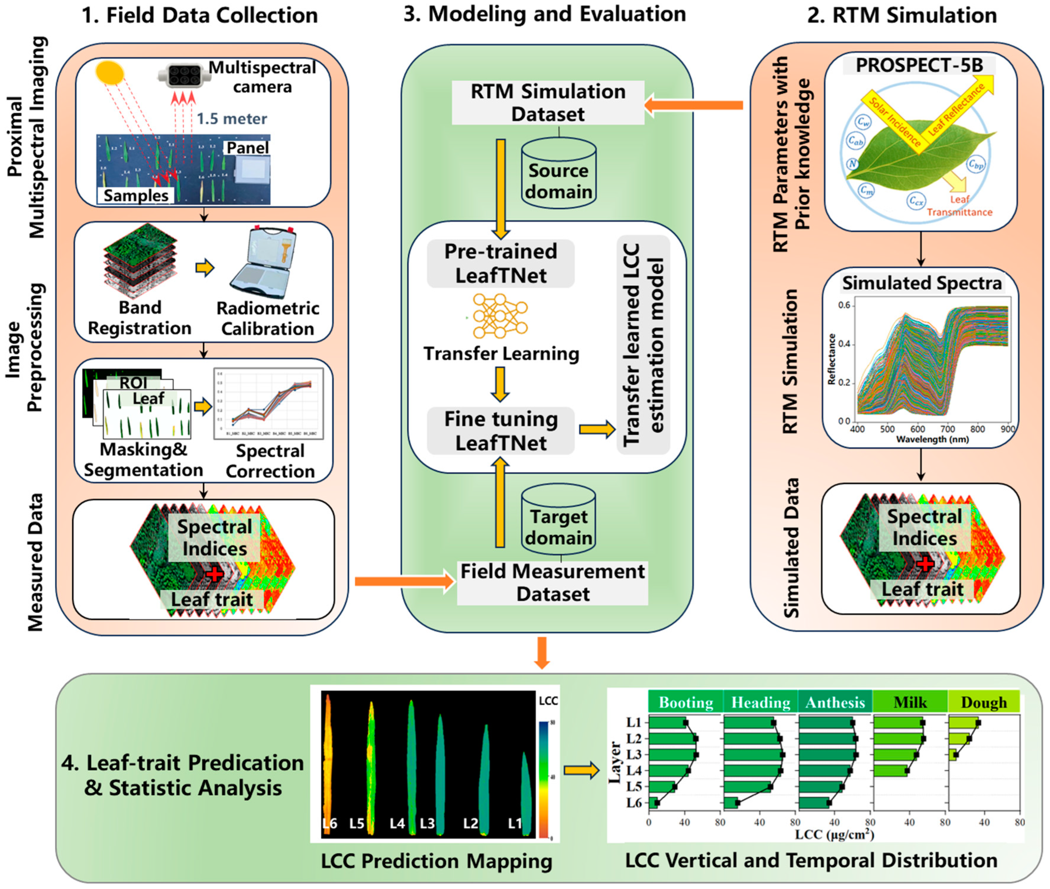
2.3. Model Establishment

2.3.1. RTM Simulation Training Dataset Generation

The PROSPECT-5B is a widely used radiative transfer model (RTM) in remote sensing to simulate leaf optical properties, providing detailed insights into light interaction with plant leaves [43]. It is an essential tool for interpreting plant leaf reflectance spectra by integrating biochemical traits and structural parameters, significantly contributing to the understanding and monitoring of vegetation dynamics. The detailed model parameter settings are shown in

Table 3. The parameters of the leaf-scale PROSEPCT-5B model.

Parameter	Symbol	Units	Range
Leaf mesophyll structure index	Nstruct	-	1.5–2.5
Leaf chlorophyll content	LCC	μg·cm−2	0–80
Leaf carotenoids content	Car	μg·cm−2	0–15
Equivalent water thickness	EWT	cm	0.001–0.1
Leaf mass per area	LMA	mg.cm−2	2–20

. In this study, a homologous transfer learning mechanism was employed, establishing a connection between the general characteristics of PROSPECT-5B simulation datasets and field measured data from proximal multispectral based on the electromagnetic physics theory of materials (Figure 2). This approach allows deep neural network trained on PROSPECT-5B simulation data to be the source of knowledge for estimating leaf traits from proximal multispectral data.

Certain input parameters of PROSPECT-5B were set to variable or constant values based on the historical data from the field measurements in the study area or existing studies (Table 3). The brown pigment content, which has a minimal impact on the spectral reflectance [44], was set to 0. The range values for leaf chlorophyll content were obtained from field measurements conducted during different wheat growth stages. To represent realistic cases, the leaf structure index, leaf carotenoid content, leaf equivalent water thickness, and leaf dry matter content were derived from related studies [45,46].

A random Latin hypercube sampling design was employed to evenly populate the canopy realization space. Finally, a total of 30,000 instances of spectral reflectance and associated biochemical traits were produced. To match the broadband wavelength of proximal multispectral, the simulated spectral data were resampled. The corresponding vegetation indices, as mentioned in Table 2, were generated from the original LUT tables to construct the final RTM-based synthetic dataset, which are used as pre-training dataset in the modeling process.

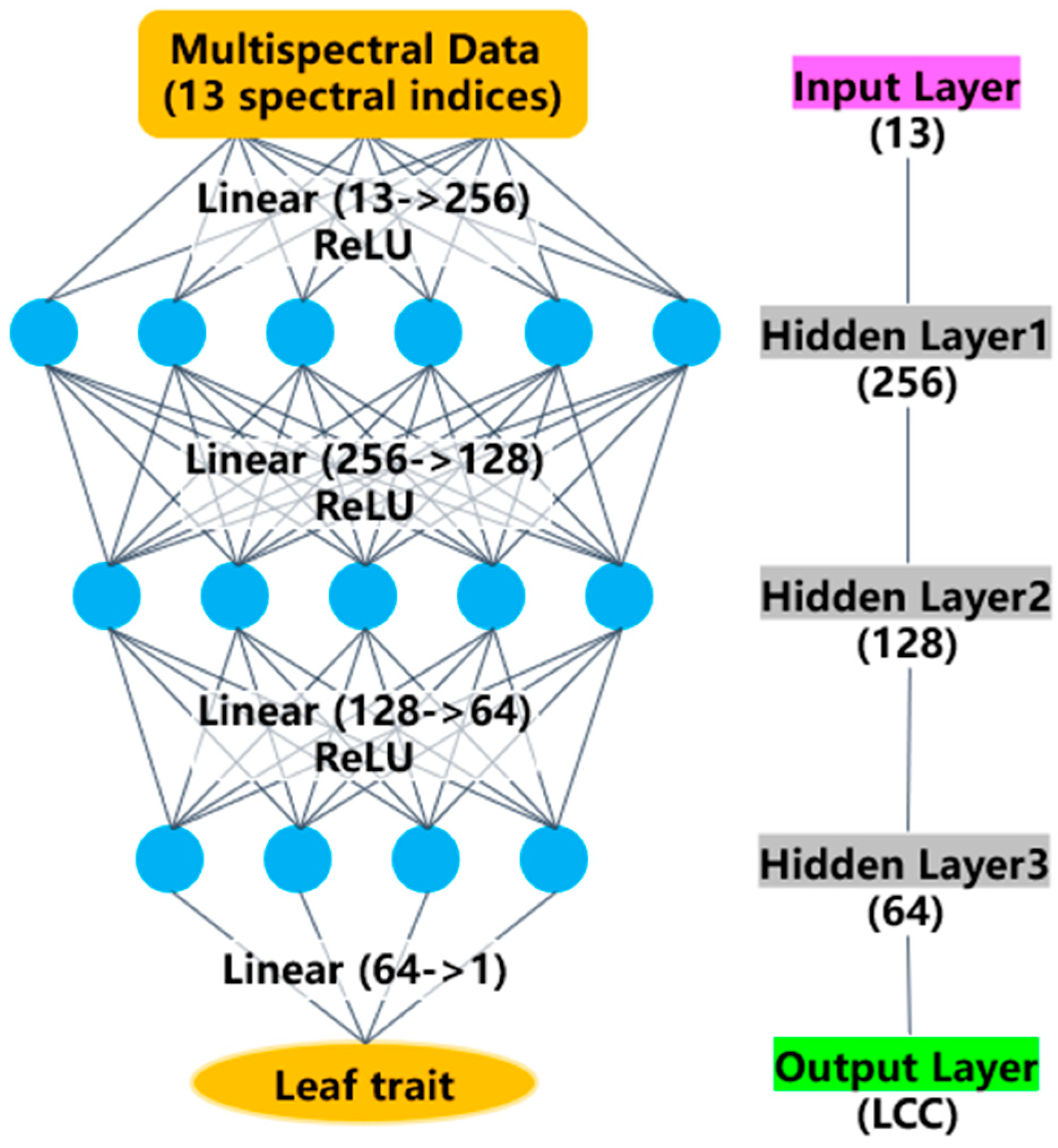
2.3.2. LeafTNet Based on Tapering Network Concept

Spectral variables and leaf traits exhibited complex relationships, involving multicollinearity and data redundance. Deep learning uses multiple hidden layers for feature extraction. A deep neural network was developed in this study using a four-layer fully connected tapering network architecture to analyze the 1D spectral data (Figure 3). Each layer employed the linear transformation. Subsequently, introducing nonlinearity with the Rectified Linear Unit (ReLU) activation function to each hidden layer, enabling the network to learn and represent complex nonlinear relationships. The final output layer omitted ReLU to maintain continuous output values suitable for the regression task. The hidden units were configured in descending order as 256, 128, and 64, which facilitates progressive feature compression and reduces reliance on noisy or irrelevant features. The tapering network architecture in deep neural networks gradually compresses low-level features into higher-level abstract features, thereby reducing redundant information and extracting more meaningful feature representations. By limiting the capacity of subsequent layers (with fewer nodes), the network selectively preserves and transmits the most important information, which helps to reduce the complexity of the model, lower computational complexity, thereby reducing the risk of overfitting.

2.3.3. Model Training

The general process of transfer learning involves fine-tuning a complex pre-trained neural network model from the RTM-based synthetic simulations, by re-training the model using a few labeled field data to improve the performance of target tasks (Figure 2). Since the pre-trained model is based on RTM-based synthetic simulations (source domain), it can efficiently adapt to the target domain (proximal field data) through fine-tuning [47]. We evaluated LeafTNet to develop the transfer learning model.

(1)

Pre-Training of the LeafTNet Network

In the model implementation, the procedure commenced with a pre-trained LeafTNet Network using PROSPECT simulation data, followed by fine-tuning using the labeled field data. Given the regression characteristic of the task, the loss function used was mean squared error. For the pre-training phase, simulated data comprising 300,000 records was partitioned into training, validation and test sets in a ratio of 3:1:1. A batch size of 500 and epoch count of 300 were specified. The ‘Adam’ optimizer was utilized with an initial learning rate of 0.001, reduced by a factor of 0.2 if the epoch count exceeded 100 iterations. Furthermore, early stopping criteria were implemented to halt training automatically if the loss function did not decrease by at least 1 × 10⁻⁴ within 30 epochs.

(2)

Fine-tuning of the LeafTNet Network

During the fine-tuning phase, the field measured data were divided into training and testing sets using a 7:3 split ratio, ensuring the independence of testing data from the fine-tuning process. The field measurements were partitioned according to the wheat growth stages. The architecture of the model was frozen, focusing solely on adjusting network parameters. Batch sizes of 16 and 300 epochs were employed. To mitigate issues of overfitting or underfitting, the early stopping criteria similar to those used in the pre-training stage were implemented. Furthermore, a 5-fold cross validation was conducted during fine-tuning to optimize the model parameters on the training set. Finally, the performance of the fine-tuned model was assessed using the testing set to evaluate its accuracy.

2.4. Statistical Regression Approach

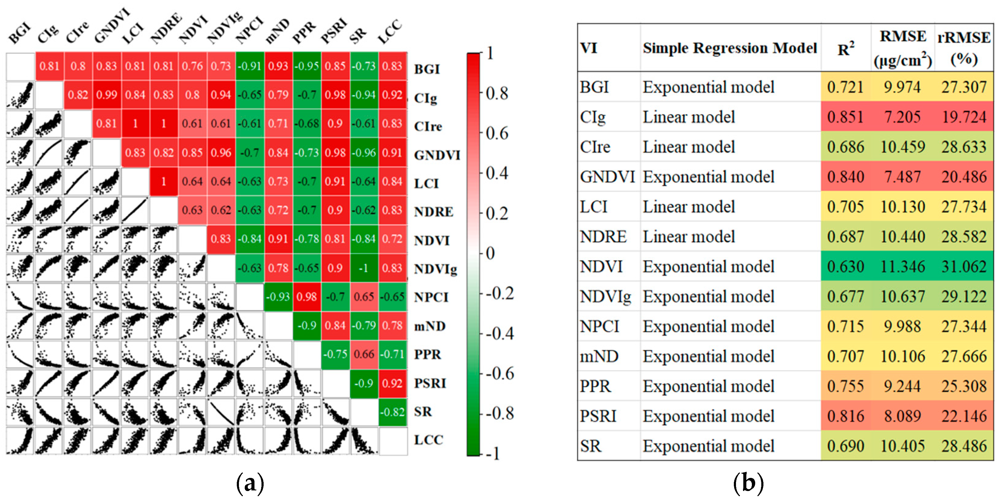
2.4.1. Empirical Statistical Model Based on Spectral Index

Empirical statistical models were generally used to establish a linear or nonlinear regression relationship between VIs and leaf traits, owing to their simplicity and practical applicability. The commonly used VIs (Table 2) related to LCC were selected to construct the regression models. The linear and nonlinear models of VIs and LCC were established using the least squares method and generalized linear model with the Poisson distribution term, respectively.

2.4.2. Partial Least-Squares Regression

PLSR is a popular statistical machine learning method for constructing a nonparametric predictive model when data exhibit high dimensionality and multicollinearity. PLSR combines features of principal component analysis and multiple linear regression, making it a valuable tool in exploratory data analysis and predictive analytics. In this study, to determine the number of factors used in the PLSR model, repeated k-fold cross validation was used to compute the root mean square error.

2.5. Model Evaluation

The LeafTNet model was implemented and evaluated using the PyTorch framework. The dataset was divided into training and testing sets using a 7:3 split ratio for all modeling methods in this study. To ensure consistency across model evaluations, a fixed random seed was employed during data partitioning, ensuring that all models utilized identical training and testing datasets for fair performance comparisons. Model accuracy was evaluated using three standard metrics: coefficient of determination (R²), root mean squared error (RMSE), and relative root mean squared error (rRMSE).

$${\mathrm{R}}^2=1-{\displaystyle \frac{{\displaystyle {\sum }_{i=1}^n{(y_i-Y_i)}^2}}{{\displaystyle {\sum }_{i=1}^n{(y_i-\overline{Y})}^2}}},$$

(4)

$$\mathrm{RMSE}=\sqrt{{\displaystyle \frac{1}{n}}{\displaystyle {\sum }_{i=1}^n{(y_i-\overline{Y})}^2}},$$

(5)

$$\mathrm{rRMSE}={\displaystyle \frac{\mathrm{RMSE}}{\overline{Y}}}\times 100,$$

(6)

where n is the number of samples, y_i refers to the ith predicted value, Y_i represents the ith measured value, and $\overline{Y}$ is the average measured value.

3. Results

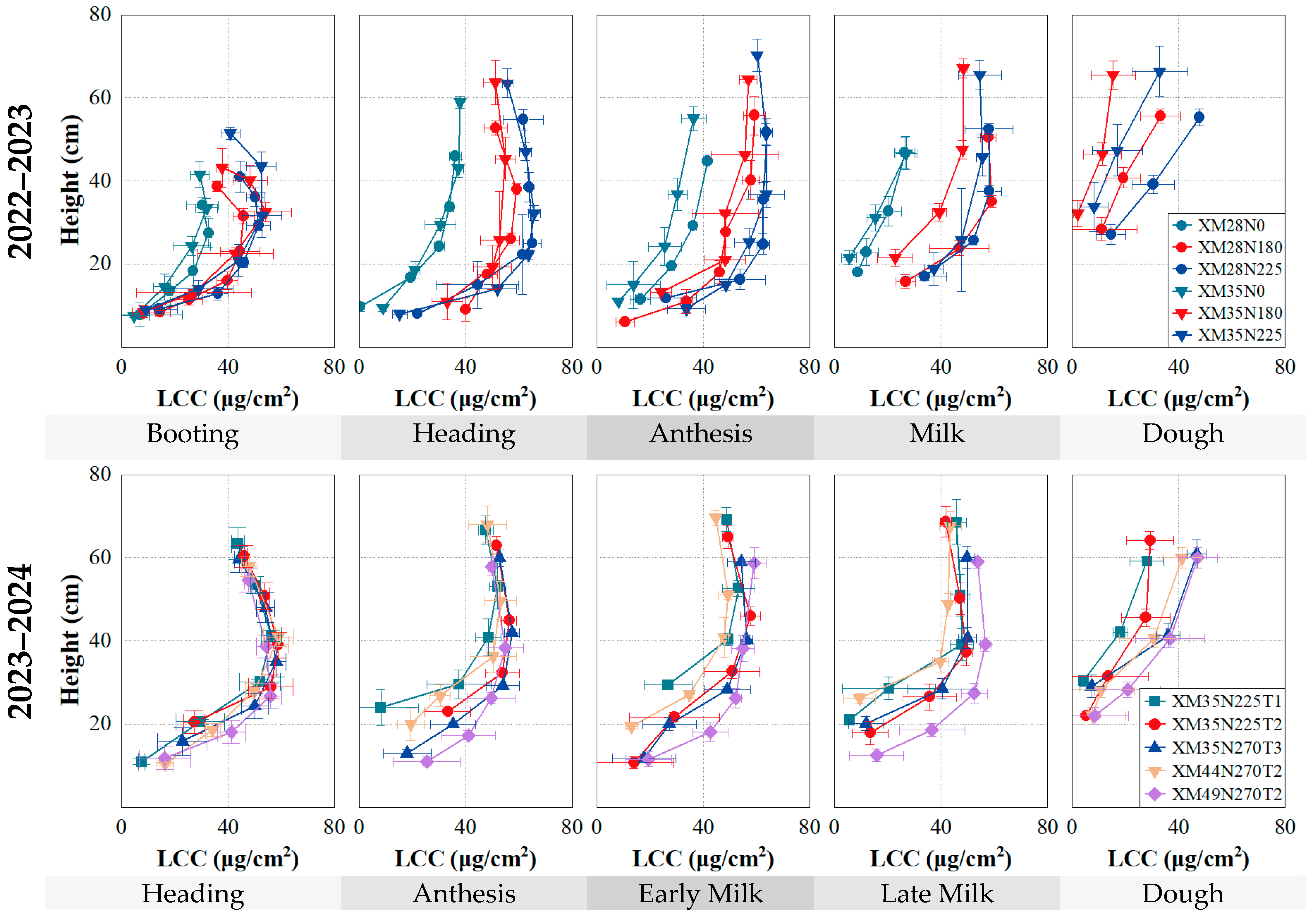
3.1. The Vertical and Temporal Variations of LCC within Winter Wheat Canopies

The vertical profiles of leaf chlorophyll content (LCC) within wheat canopies at various growth stages were investigated and are presented in Figure 4. In these cases, the height of each leaf collar above the ground was referred to as the height of the leaf layer within the canopy. Additionally, it should be noted that only the green leaves within the canopies in this study were used to determine the chlorophyll content, as the withered and yellowed leaves were brittle and wrinkled and thus difficult to quantify.

As shown in Figure 4, the measured LCC showed different vertical profiles within the wheat canopies across the growth stages under various N treatments. Under nitrogen-deficient treatment, the gradient of the vertical distribution of LCC was steeper. During the early reproductive growth period (booting stage), the vertical profile of LCC exhibited a pronounced bell-shaped pattern. Specifically, LCC values were lower in the bottom layer, increased in the middle layer, and then decreased in the upper layer. As the growth season progressed, the difference in LCC between upper and middle leaves decreased, eventually presenting a monotonically increasing pattern from the bottom to the top layers during the later reproductive growth period (dough stage). The results indicated that different growth stages and nitrogen treatments were associated with changes in the vertical distribution of LCC within the canopies. Under high N treatments, LCC exhibited an evolutionary process from the form of non-monotonic curves in the early reproductive growth period to the form of monotonic curves in the later period with height variation. Although there was no regular fertilization gradient during the 2023–2024 growth season, it involved multiple wheat varieties, which further confirmed the vertical and temporal variation characteristics of wheat LCC. Overall, these provided convincing evidence for the notable variation in LCC traits found within winter wheat canopies under different growth stages and N treatments.

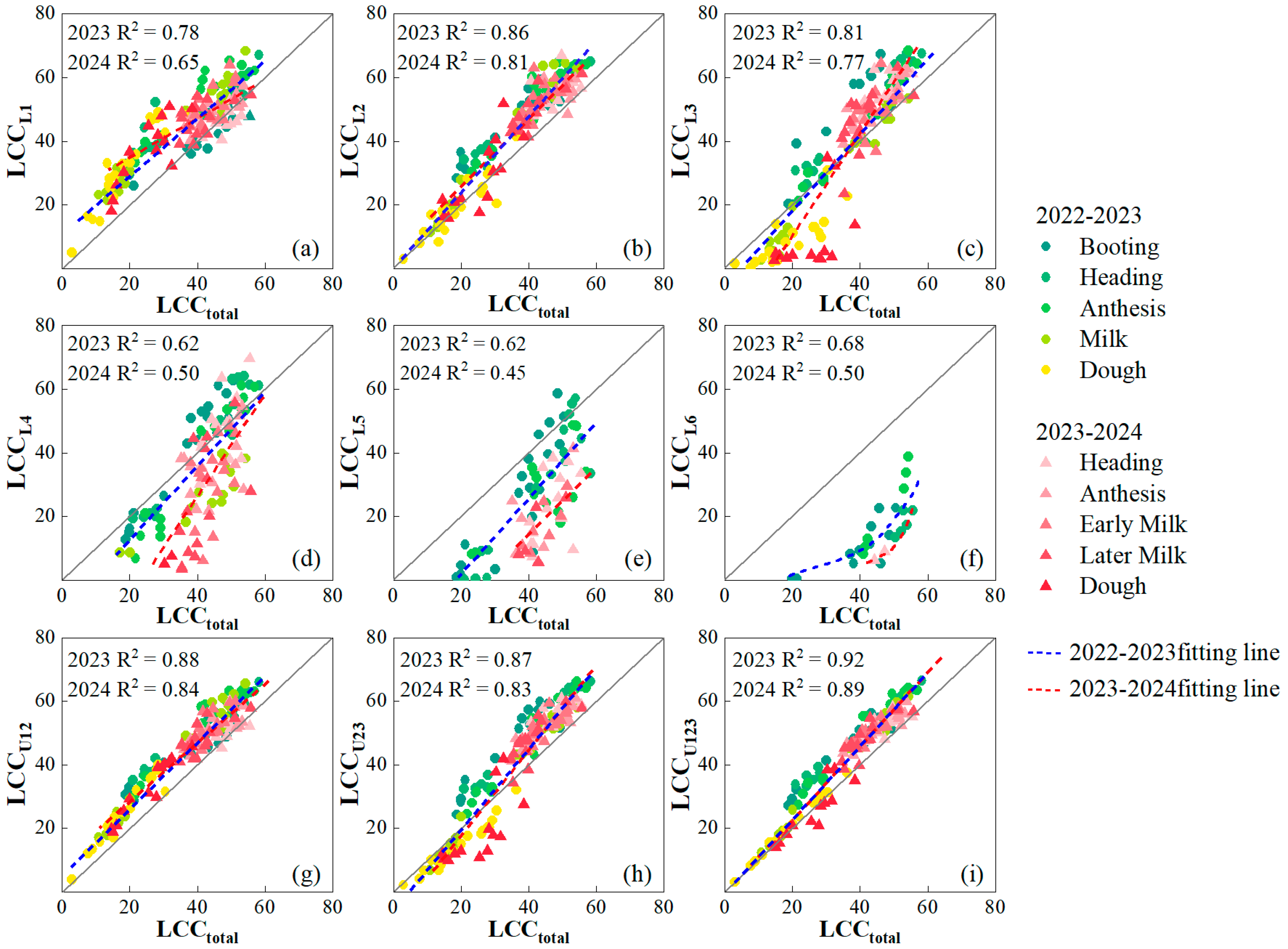
3.2. The Relationship of LCC_total with LCC_Li,_Ui

LCC_total is the accumulation of LCC × LA by individual vertical layers, which represents the LCC of the entire canopy. Figure 5 shows the relationship between LCC of different leaf layers and LCC_totol. For single-layer LCC_Li, the rank of determination coefficients (R²) was: LCC_L2 > LCC_L3 > LCC_L1 > LCC_L5 > LCC_L4 > LCC_L6. Compared to the LCC in the lower layers (LCC_L3-L6), the correlation between LCC_total and LCC in the upper layers (LCC_L1-L3) was more significant. For multi-layer LCC_Ui, the rank of R² was LCC_U123 > LCCU₁₂ > LCC_U23. Note that the slope of the fitting lines about LCC_U12 and LCC_total is closest to 1, indicating that LCC_U12 was more consistent with the changes in LCC_total. Therefore, LCC_U12 was the most representative of LCC_total for evaluating canopy chlorophyll status during the entail growth season. These results can also provide important reference for the selection of leaf samples for ground sampling in canopy remote sensing observations.

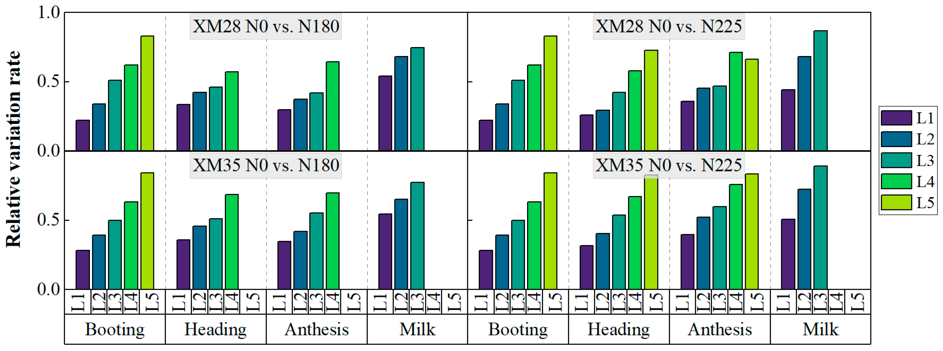
3.3. Effects of Different Nitrogen Fertilization Treatments on the LCC_Li

LCC-based nitrogen use efficiency (relative variation rate) was employed using the analogous computational procedure as in [48]. Figure 6 shows the relative variation rates of the LCC_Li in response to different nitrogen fertilization treatments. The results indicated that the effects of N rates on LCC_Li increased gradually from upper to lower layers within the canopies. The effects of different N rates on the LCC_Li did not significantly differ between the two winter wheat varieties. Overall, the LCC at the bottom layer of the wheat canopy was more susceptible to the nitrogen fertilization rates. This further demonstrated the importance and necessity of estimating LCC at different vertical layers.

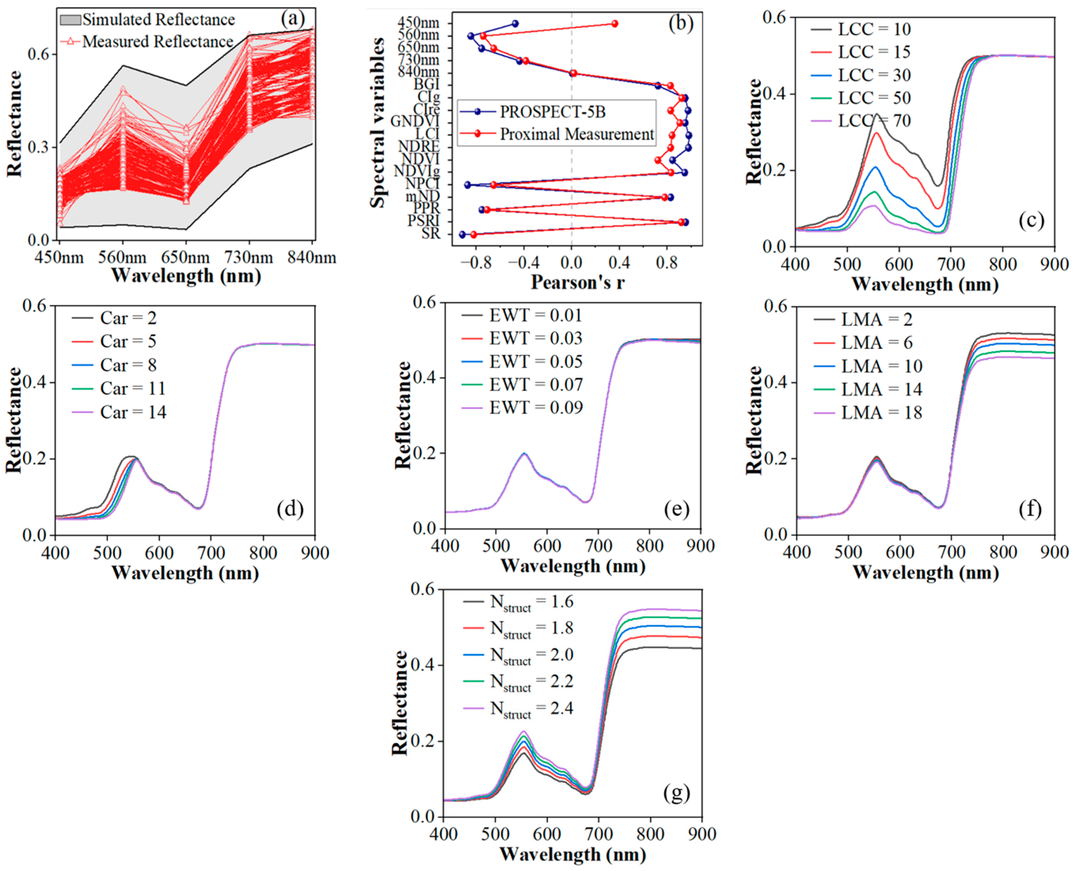
3.4. Characteristics and Sensitivity of Wheat Leaf Spectrum

All samples collected from the same N treatment were divided into various groups according to the vertical layers of the leaves. To observe the spectral response to the different leaf layers within the canopy, the LCC for each group was analyzed at each growth stage. Figure 7 shows a polygonal map representing the multispectral reflectance of the five bands that were preprocessed by MSC. The blue (450 nm), green (560 nm), red edge (730 nm), and near-infrared (850 nm) bands on the spectral reflectance curve showed the most alterations, whereas the red (650 nm) band showed no discernible changes. As LCC increased, the reflectance of the green band decreased. The characteristics of spectral bands showed changes in sensitivity at different leaf vertical layers. The observable variations in the reflectance spectrum among the vertical leaf layers demonstrated the vertical heterogeneity of the leaf traits. These results suggested that it was feasible to evaluate the LCC vertical variation based on broadband multispectral information.

Figure 8a shows the relationship between LCC and thirteen vegetation indices throughout the entire growth season. As shown in the scatter plot in the lower left of the figure, the relationship between vegetation indices and LCC can be divided into two types: linear and nonlinear. Therefore, the linear and nonlinear models of VI-LCC can be constructed using the least squares method and generalized linear model with a Poisson distribution term, respectively. We used the thirteen vegetation indices to establish the inversion model for LCC over the entire growth season. The results of thirteen VI models are shown in Figure 8b. The findings demonstrated a relatively significant linear connection between LCC and several widely used VIs, such as the Chlorophyll Index using Green Reflectance (CIg), with R² of 0.851. However, the Chlorophyll Index using Red Edge Reflectance (CIre, R² = 0.686) and the Normalized Difference Vegetation Index (NDRE, R² = 0.687) did not fare as well. Moreover, a relatively strong nonlinear correlation was found between LCC and several widely used VIs, such as the Green NDVI (GNDVI) and Plant Senescence Reflectance Index (PSRI) (R² for GNDVI was 0.840, R² for PSRI was 0.816). These VIs were derived from a combination of blue, green, and near-infrared (NIR) bands, suggesting that those bands had a decent capacity to estimate LCC under relatively complex conditions. These findings indicated that the spectral band combination of the blue, green and NIR bands derived from the broadband multispectral reflectance was crucial for LCC estimation.

Figure 9a shows 30,000 simulated spectral reflectance data generated by the PROSPECT-5B model, with the proximal measured reflectance data overlapping the range of the simulated data. Shadows indicated the range of simulated reflectance. The distribution of simulated spectra effectively encompassed most of the measured spectral reflectance of winter wheat across different growth stages, demonstrating the comprehensive coverage and representativeness of simulated spectra. As shown in Figure 9b, the correlation pattern between LCC and spectral variables of PROSPECT simulation and proximal measurement exhibited a highly similar trend. This further indicated that the simulated data and the measured data have good consistency. Vegetation indices significantly enhanced the correlation between spectra and the LCC compared to the single band. This also was the reason why vegetation indices were used as the independent variable input in this study. In addition, the correlation coefficient of PROSPECT spectral variables exhibited a slightly higher amplitude than those of proximal spectral variables.

The sensitivities of leaf reflectance within the 400–900 nm range to variations in leaf parameters are presented in Figure 9c–g. The results indicate that reflectance in the spectral range exhibited a high sensitivity to changes in LCC and N_struct, while showing low sensitivity to changes in EWT. The regions sensitive to LCC overlapped with those for Car between 450 and 560 nm. LMA showed high sensitivity in the 750–900 nm range and low sensitivity in the 550–650 nm range. LCC mainly affects the leaf reflectance in the visible light and red-edge regions, while N_struct affects the leaf reflectance of the entire spectrum regions. Consequently, these parameters must be accounted for when employing the PROSPECT-5B model to generate simulated datasets. Notably, LCC and N_struct jointly describe the photosynthesis of leaves from the absorption process and reflection process of light radiation, exhibiting coupled effects on the leaf reflectance spectrum. While winter wheat leaves generally exhibit subtle differences among various cultivars, their overall appearance and structure are quite similar. The distinctions in photosynthetic pigment contents are mainly influenced by environmental conditions such as light, temperature, and water-nutrient availability. The leaf mesophyll structure index (N_struct) reflects the complexity of the cell and pore structures inside the leaf, and related to the differences in photosynthetic efficiency and nutrient accumulation among cultivars [49,50]. A high N_struct indicates an increase in multiple reflections and scattering of light inside the leaf, resulting in an increase in spectral reflectance.

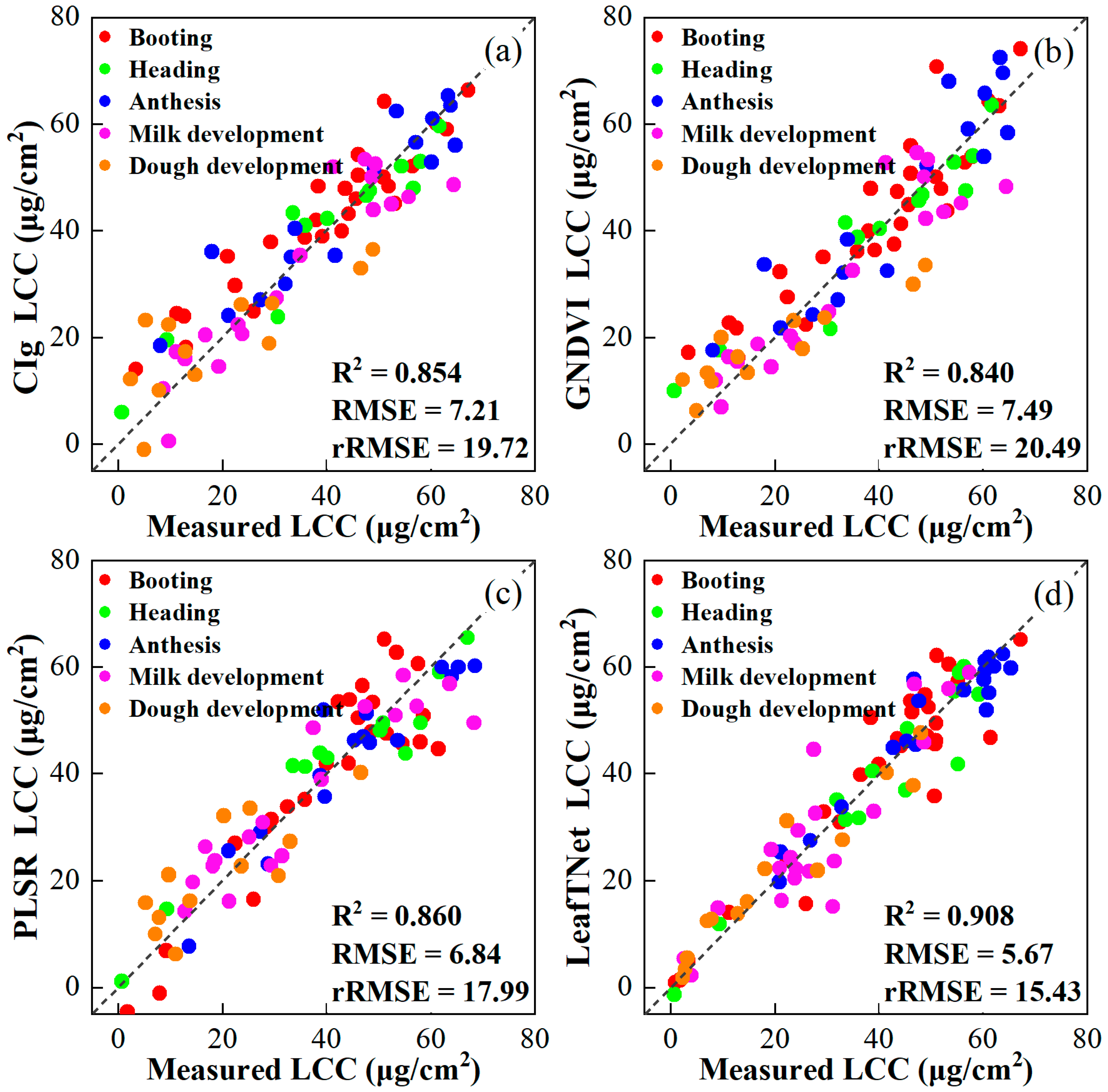
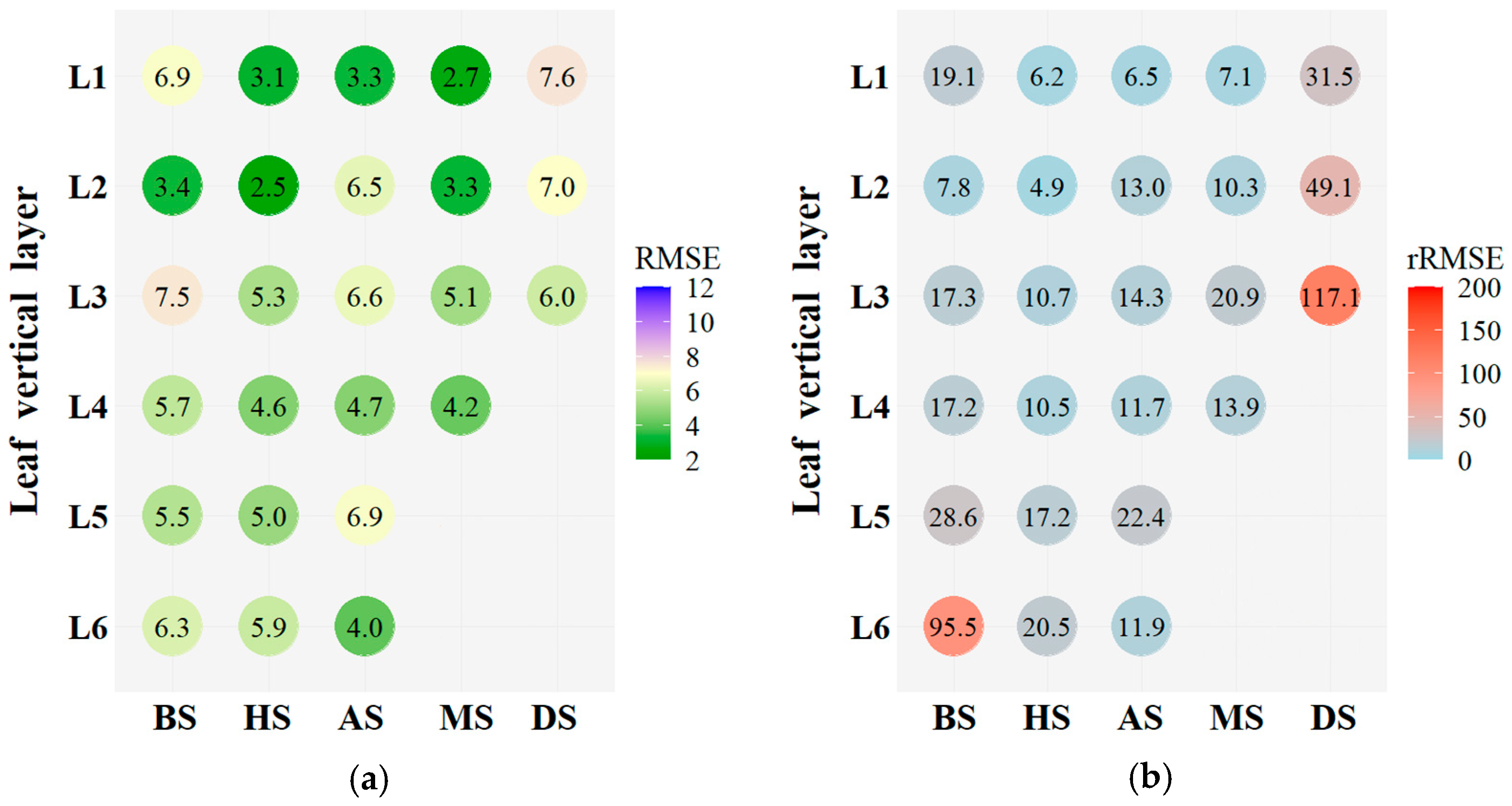
3.5. Retrieved LCC with LeafTNet and Transfer Learning

Applying transfer learning, we fine-tuned the LeafTNet for LCC retrieval using field proximal measured data. The validation results are presented in Figure 10. Additionally, the linear CIg-LCC model and nonlinear GNDVI-LCC model (chosen for having the highest estimation accuracy among the thirteen VI-LCC models) and PLSR, were compared. The results demonstrate that the transfer learning model LeafTNet can predict LCC with satisfactory performance, and it exhibited superior prediction accuracy compared to using the empirical VI-LCC methods and traditional machine learning PLSR method. Furthermore, the accuracy of LCC predictions varied across different growth stages. For the LeafTNet, the accuracy in rRMSE from highest to lowest was as follows: anthesis (R² = 0.913, RMSE = 4.235 μg/cm², rRMSE = 8.283%), heading (R² = 0.913, RMSE = 5.001 μg/cm², rRMSE = 11.640%), booting (R² = 0.869, RMSE = 6.255 μg/cm², rRMSE = 14.141%), milk development (R² = 0.854, RMSE = 5.540 μg/cm², rRMSE = 24.471%), and dough development (R² = 0.773, RMSE = 6.949 μg/cm², rRMSE = 21.275%). Overall, the LCC prediction accuracy was higher during the early reproductive growth period and lower in the later period. Variations in leaf component and structure may be the main reason for the differing prediction accuracy. As the leaves senesce, chlorophyll content decreases and becomes non-uniformly distributed on the leaf surface, significantly affecting the measured data and thereby interfering with the estimation results.

3.6. Visual Mapping of LCC Trait

As shown in Figure 11, the maps of LCC distribution in wheat leaves at different vertical leaf layers during various growth stages were produced by applying the LeafTNet model to the proximal multispectral images. The maps present the spatial and temporal distribution of LCC of winter wheat. When combined with further statistical analysis of predicated pixel values for different leaf layers, as employed in Section 3.1, these maps can help us to detect the subtle change in LCC in wheat leaves at different vertical layers during various growth stages and nitrogen treatments. The exploration of LCC at a fine scale contributes to a more nuanced understanding of the growth status of various functional leaf layers and implications for the identification of stressors or nutrient deficiencies. Based on proximal multispectral imaging data, the LeafTNet offers an effective solution for estimating vertical and temporal variations in wheat leaf chlorophyll content.

4. Discussion

4.1. Vertical Distribution of LCC within the Winter Wheat Canopies

Previous studies indicated that the vertical distribution of LCC within the canopy exhibited non-uniformity, with lower shaded leaves typically having lower LCC than upper sunlit leaves [14,51,52]. In this study, we investigated the vertical and temporal distribution characteristics of LCC in winter wheat canopies across different growth stages and under various nitrogen fertilizer treatments. Our findings revealed that the LCC values of upper leaves were not consistently higher than those of lower leaves. Furthermore, the vertical LCC profile of winter wheat varied throughout the growth season and was also affected by N fertilization treatments.

The vertical profile of winter wheat LCC exhibited dynamic changes during the entire growth season. Unlike corn, where grain development occurs in the middle of canopy and the vertical LCC profile remains relatively stable with a bell-shaped distribution [53], the vertical LCC profile of winter wheat changed continuously throughout the growing season (Figure 4). During the early reproductive growth period (booting and heading), wheat LCC displayed a bell-shaped distribution, with lower LCC in the young upper leaves and senescent bottom leaves, while higher LCC was observed in the mature middle leaves. As the growth season progressed, the LCC difference between upper and middle leaves decreased, eventually presenting a monotonic distribution during the later reproductive growth period (dough stage). This shift can be attributed to the interaction between light adaptation and nutrient competition. The upper sunlit leaves receive more intense light radiation and are allocated more nutrients for chlorophyll synthesis to maintain the metabolic balance, while absorbing foliar nutrients from the lower leaf layers [54]. Crops respond to light stress by altering chlorophyll in different vertical leaf layers to maintain photosynthetic efficiency. Additionally, due to the transferability of nitrogen within crops [55], nitrogen stored in the leaves is mobilized and transported from lower leaf layers to support the developing grains at the top of the wheat canopy [20,56,57]. Consequently, during the late reproductive growth period, upper sunlit leaves still maintain a higher chlorophyll synthesis capacity than that of lower shaded leaves, owing to transported nitrogen supply and stronger light radiation.

The analysis results of LCC-based nitrogen use efficiency (Figure 6) indicated that LCC response to nitrogen fertilization rates varied across different vertical leaf layers, with lower leaf layers being more susceptible to nitrogen rates than upper layers. Chlorophyll, a crucial photosynthetic pigment, is closely linked to plant nitrogen levels, as nitrogen is a key component of chlorophyll molecules. Previous research has suggested that the effect of varying nitrogen rates on the leaf nitrogen concentration (LNC) became more pronounced from the top to the bottom of the crop canopy [9]. Within the wheat canopy, nitrogen is non-uniformly distributed, with a preferential allocation to upper, younger leaves due to their higher photosynthesis contribution. Consequently, lower leaves in shaded environments, which receive less priority for nitrogen allocation, are more prone to deficiency symptoms and a more significant decline in chlorophyll content. These environments make LCC in lower layers more susceptible to nitrogen fertilization treatments. Additionally, research demonstrates that the fraction of photosynthetically active radiation intercepted (FIPAR) of the upper layers of winter wheat was especially more susceptible to nitrogen rates than that of lower layers [17], exhibiting a contrary pattern compared to LCC response. Under sufficient light radiation conditions, plants optimize photosynthesis by adjusting leaf morphology and physiological processes, potentially leading to increased chlorophyll synthesis in the upper sunlit leaves and reduced nitrogen demand in shaded lower leaves. This adaptation further contributes to LCC in lower layer being more susceptible to nitrogen fertilization. Overall, the variability of vertical LCC response to nitrogen application is caused by the interaction between light adaptation and nutrient competition. The heightened sensitivity of LCC in the lower leaves to nitrogen fertilization could offer valuable opportunities for the timely diagnosis of the nitrogen nutritional status of winter wheat and further improve crop management.

Given the labor-intensive and time-consuming nature of traditional laboratory biochemical analysis, future studies could utilize handheld chlorophyll content meter devices for rapid sampling and measurements of LCC in different vertical leaf layers. Additionally, incorporating crop vertical stratification into remote sensing techniques can be used to obtain more accurate and comprehensive data on crop characteristics and enhance the efficiency and effectiveness of agricultural research and management. By accurately capturing the spatial and temporal variability of crop layers, researchers can make informed decisions to optimize agricultural practices and improve crop productivity, resource use efficiency, and sustainability.

4.2. Influencing Factors on Winter Wheat LCC_Li Estimation Using Proximal Imaging Data

In contrast to canopy-level remote sensing observations, which are susceptible to multiple factors such as soil background, multiple scattering, and crop phenotypic conditions that can significantly interfere with prediction results [20,50], leaf-scale observations facilitate more precise measurements through direct interaction with individual leaves, thereby avoiding the confounding effects encountered at the canopy-level. Consequently, leaf-scale observations are particularly valuable for detailed studies of crop traits at a fine scale. Nevertheless, several factors can still affect the estimation accuracy and consistency of leaf-scale measurements using proximal multispectral imaging data. (i) Spectral data preprocessing: leaf reflectance collected under natural solar lighting conditions may exhibit inherent spectral response inconsistencies due to the changes in solar altitude angle and leaf inclination angle, leading to baseline drift in the spectral data. In this study, data processing was employed using multiplicative scatter correction (MSC) to ensure spectral consistency, and enhance the correlation between spectra and laboratory data. The normalization process inherent in MSC can also help mitigate the vignetting effects caused by non-uniform illumination across the camera’s field of view. Since MSC adjusts both the baseline and the scale of each spectrum, it can reduce the impact of light intensity variations, leading to more consistent reflectance measurements. (ii) Leaf age and growth stage: the canopy comprises distinct vertical layer leaves at varying growth stages, including young, mature, and senescent leaves. In mature leaves, the cellular structure and function are relatively intact, with chlorophyll typically distributed uniformly across the leaf surface. However, in senescent leaves, the distribution of chlorophyll is often non-uniform. Some areas may exhibit significantly lower chlorophyll content or even a complete absence of chlorophyll, while other regions might still retain some chlorophyll. Measurement difficulties arise when assessing LCC in the senescent leaves, leading to potential errors that adversely affect LCC estimation.

To further validate the relationship between leaf spectral modeling and the vertical distribution of LCC during the growth season, the LeafTNet model was performed to predict LCC under different vertical and temporal conditions (Figure 12). The average image pixel values of predicted LCC were extracted using the ArcGIS Zonal Statistics Tool. RMSE was used to intuitively measure the prediction accuracy of each vertical layer in this study. Considering the variability in the range of LCC among different vertical layers, rRMSE more effectively reflects the generalization ability of the models across different vertical layer datasets. The inversion performance of the model varied with the vertical leaf layer. The rRMSE values of upper layers generally exhibited higher accuracy than those of lower layers at the same growth stage. Additionally, the model exhibited higher performance during the mid-reproductive growth period, while the performance was less favorable at the early and later mid-reproductive growth periods. During the mid-reproductive growth period, all leaves within the wheat canopy were at an intact functional level, and the model can accurately predict the leaves of all layers in the canopy. In contrast, the physiological functions of leaves weaken at the late reproductive growth period and LCC non-uniformly distributed on the leaf surface, which affect data measurement, thereby interfering with the estimation results based on spectral information.

4.3. Feasibility of Transfer Learned LeafTNet

Using simulated data generated from physical radiative transfer models to pre-train the LeafTNet, followed by fine-tuning with field-measured data, presents an effective alternative to collecting and labeling measured data. Simulated data can be produced rapidly and involve various environmental conditions that are not easily captured in real-world scenarios. This approach reduces the need for extensively labeled and sample measurements in the pre-training process. Therefore, the highly efficient LeafTNet, integrating transferred knowledge and the finetuning process, is very necessary and needs to be explored in crop leaf trait estimation.

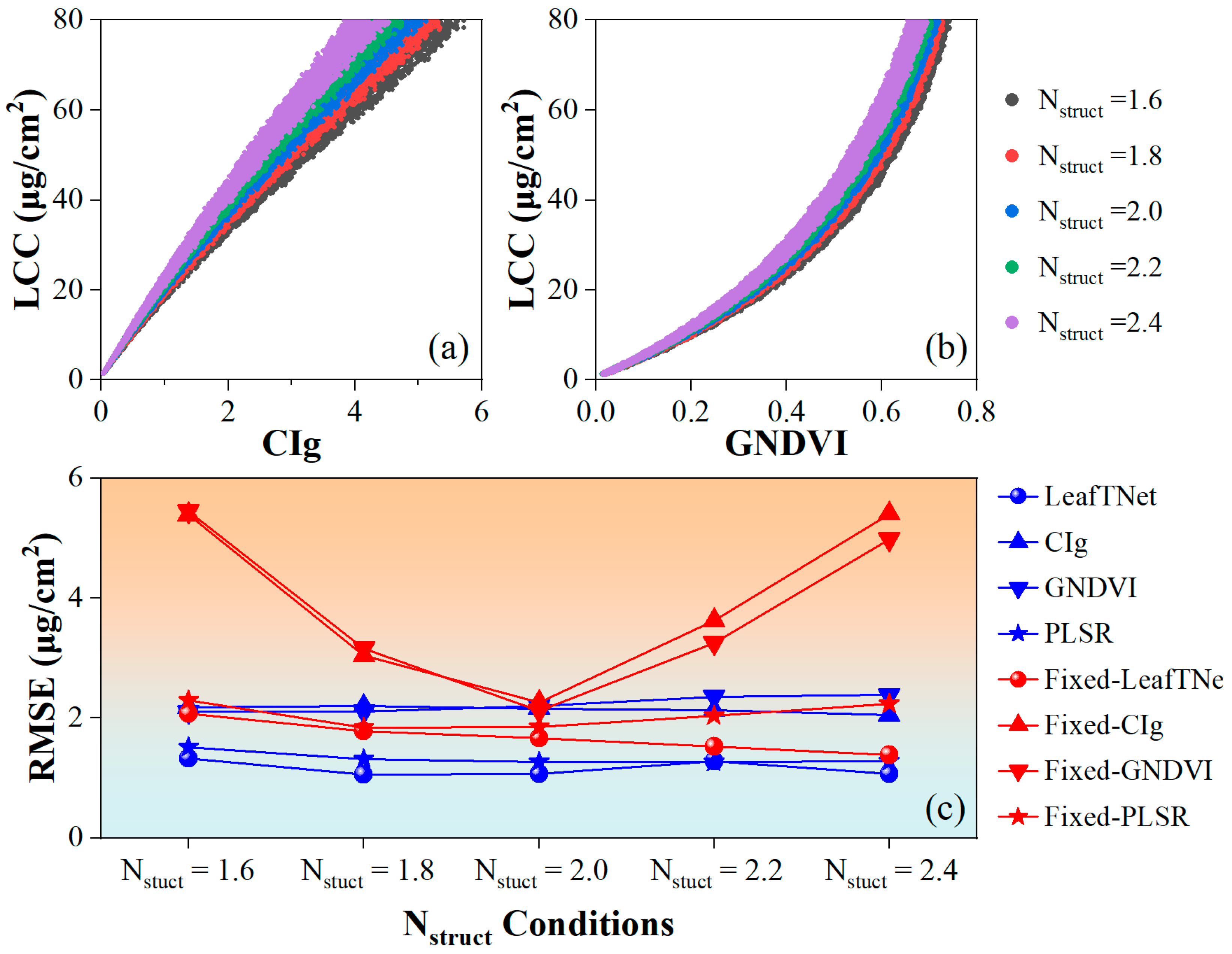
4.3.1. Sensitivity of LCC Inversion to N_struct Vatiation

The universality of the trained LeafTNet model depends on the representativeness of the dataset used for modeling. If the dataset covers various possible conditions in the target application context, the model is likely to perform well on other similar datasets. In this study, the leaf-scale radiative transfer model PROSPECT-5B was utilized to simulate data under different conditions. The spectral variables from the simulated data were then used for modeling to test the model’s generalization ability. The previous experimental results indicate that LCC and N_struct have significant coupling effects on the leaf reflectance spectrum (Figure 9). Therefore, it is necessary to investigate the LCC estimation performance of LeafTNet as N_struct changes.

To investigate whether N_struct variations affect the accuracy of LCC retrieval using LeafTNet model, 7 sets of 30,000 simulated data points with different N_struct conditions were utilized. Initially, LCC was retrieved under specific N_struct condition. Additionally, the linear CIg-LCC model and the nonlinear GNDVI-LCC model, chosen for their highest estimation accuracy among the thirteen VI-LCC models, and machine learning method PLSR, were compared. The results suggest that all these models achieved high and stable prediction accuracy (as shown with the blue lines in Figure 13c). In order to further assess the resistance of each model to N_struct influences in the LCC retrieval process, the model trained from the data pool with mixed N_struct values (including the entire simulated data) was used as the fixed model to retrieve LCC under certain N_struct condition varying from 1.6 to 2.4 (as shown with the red lines in Figure 13c). Due to the differences in data distribution under different N_struct conditions, the fixed VI-LCC models established using the mixed dataset exhibited unstable estimation results on specific N_strcut datasets. The results indicate that the N_struct variations significantly impacted the accuracy estimated with RMSE of the VI-LCC models. Although the LeafTNet model had a slight impact on the LCC retrieval across different N_struct conditions, it was found that LCC retrieval based on LeafTNet model achieved higher accuracy across varying N_struct conditions compared to the VI-LCC and PLSR methods.

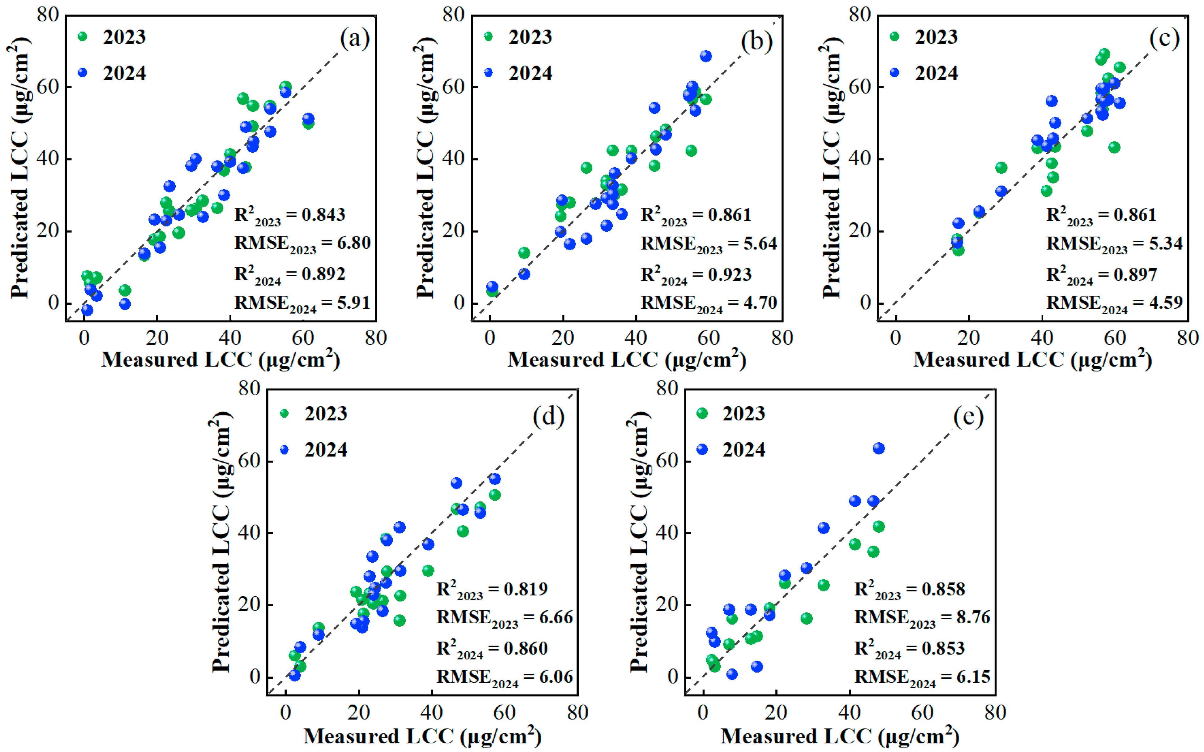
4.3.2. Annual Transferability of the Deep-Learning-Based LeafTNet

The LeafTNet model was further validated for its universality and prediction accuracy by applying the model pre-trained on the PROSPECT simulation dataset to predict LCC of the corresponding stage in 2024. The model was fine-tuned using field-measured data from the corresponding or adjacent growth stage in 2023. Additionally, the model was pre-trained using the PROSPECT simulation dataset, and then fine-tuned with field-measured data from the same stage in 2024. The results of these experiments are presented in Figure 14.

Annual transferability testing was conducted by using a model suitable for LCC estimation in 2023 to directly predict LCC in 2024. While the accuracy of the annual transferred model decreased compared to the model fine-tuned with data from the same time, it still demonstrated relatively acceptable performance in field LCC prediction. Despite the similarity in growth conditions and disturbance factors of crops in different years, they are not completely the same during the same phenological phases. Therefore, the model applicable to LCC inversion in 2023 was found to be effective for LCC inversion in 2024, highlighting the annual transferability of the proposed method and confirming the generality of transfer learning techniques based on the LeafTNet model and fine-tuning processes. This hybrid approach also shows promise for extension to other applications in the future.

The basic LeafTNet network trained on the PROSPECT simulation dataset was transferred to the LCC inversion task measured in the field and was fine-tuned using some labeled field data. Figure 10 and Figure 13 showed that LeafTNet achieved satisfactory LCC validation accuracy across different conditions, including various wheat varieties and phenological periods. These results demonstrated that the transfer knowledge extracted from the simulated dataset can expand the size of the training set, avoid overfitting, and improve the stability of the model. The fine-tuning process, incorporating specific information from the target task, accounts for specific growth conditions and uncertainties to enhance the accuracy of LCC prediction in field measurements.

4.4. Limitations and Prospects

This study demonstrated the applications of proximal multispectral imaging remote sensing for predicting LCC across vertical layers and phenology for winter wheat monitoring at leaf-scale. The findings provide a theoretical basis and technical support for monitoring growth-related leaf traits using proximal multispectral imaging remote sensing technology. However, there are still some limitations. (1) Winter wheat leaf samples were measured using a proximal multispectral camera under solar light conditions in this study. This approach improved experimental efficiency and reduced costs. However, since solar illumination condition and spectral characteristics can be affected by environmental factors, such as solar zenith angle and cloud coverage, the spectral data collected at different times may be subject to inconsistent lighting conditions. To address this, each proximal campaign was conducted at noon under a clear sky when solar illumination conditions were relatively stable. Additionally, spectral correction was performed using the multiplicative scatter correction (MSC) method to mitigate spectral drift issues from data collected at different times. Future research should consider using artificial light sources in indoor settings to provide stable and controllable lighting conditions, which would enhance experimental reproducibility and data consistency. (2) This study explored the use of a multispectral camera, originally designed for UAV platforms, as a ground-based device for leaf spectral measurements and demonstrated its feasibility for monitoring wheat leaf traits. However, there is currently a lack of automated data processing software or programs capable of performing high-quality band registration for single-frame images captured using proximal multispectral imaging. As a result, the most time-consuming aspect of the data preprocessing process is the semi-automatic geometric correction and band registration of these single-frame images. (3) This study found variability in the response of LCC to nitrogen fertilization rates across different vertical leaf layers, with the lower layer LCC being more susceptible to N rates than the upper layer. It provides additional opportunities for timely diagnosing the nitrogen nutritional status of winter wheat by monitoring vertical LCC distribution. However, the finding was investigated in limited specific wheat varieties and nitrogen rates in this study. More wheat varieties and nitrogen fertilization gradient conditions should be considered to further validate variability regarding the response of vertical LCC to nitrogen fertilization rates in order to fully explore the potential of utilizing the characteristic of LCC response to N rates for the early diagnosis of nitrogen nutritional status. (4) The proposed transfer learning LeafTNet utilized a physical radiative transfer model to provide source domain knowledge for the target task. However, reliance on PROSPECT simulation data restricts this method’s extended applicability for estimating additional biochemical components beyond those explicitly modeled in the PROSPECT model, such as nitrogen, protein, and ChlF. Indirect measurements [58,59] and modified radiative transfer models [60,61] could help overcome this limitation. (5) The destructive sampling of wheat leaves from various vertical layers, arranged horizontally for observation, enabling the effective distinction and recording of leaf layer positions, without the impacts of leaf occlusion and confounding effects encountered in the observations at canopy-level. However, the spectral data acquired at the leaf scale only capture leaf surface information and lack real spatial details of canopy structure. Future research should consider integrating three-dimensional (3D) modeling and multispectral imaging technologies to monitor the 3D variations in leaf traits within the crop canopy [62].

5. Conclusions

This study investigated the vertical distribution characteristics of LCC within winter wheat canopies across various growth stages. To effectively utilize multispectral RS information to accurately quantify winter wheat LCC at a leaf scale, a hybrid LCC inversion method was developed that integrates transfer knowledge from PROSPECT simulations and refined LeafTNet architecture. This proposed method was thoroughly analyzed and validated against both field measurement and the PROSPECT simulation dataset. The main findings of the study are as follows:

The vertical variations of LCC within the winter wheat canopy were presented in detail. It was demonstrated that the vertical profile exhibited variation throughout the growth season. During the early reproductive growth phase, LCC values were lower in the bottom layer, increased in the middle layer, and then decreased in the upper layer. As the growth season progressed to the late reproductive growth phase, LCC displayed an upward trend from the lower to upper layers within winter wheat canopy. Additionally, the results indicated that the LCC values of the wheat canopy cannot be reliably determined solely from the measurements of individual leaves, such as the flag leaves or bottom leaves, due to significant variability among different vertical layers. Moreover, it was found that LCC in the bottom layers was more susceptible to nitrogen rates than that in the upper leaf layers. It provides a potential opportunity for promptly diagnosing the nitrogen nutritional status of winter wheat by monitoring vertical LCC distribution. These results highlighted the significance of the vertical stratification of crops in remote sensing analysis to improve the accuracy and reliability of crop monitoring.

By integrating the advantages of deep learning and physical radiative transfer simulations, LeafTNet proves highly effective in remote-based leaf trait retrieval. The LeafTNet achieved notable accuracy in leaf-scale LCC estimation, outperforming traditional empirical statistics and machine learning methods that rely solely on field-measured information. Moreover, the model’s application for LCC prediction in 2023 also performed effectively in the corresponding stages in 2024. Overall, LeafTNet demonstrated robust performance and generalizability in LCC estimation of winter wheat leaves from proximal multispectral imagery. This study offers technical support for predicting the vertical LCC distribution of winter wheat leaves and provides some insights for studying the relationships between the vertical heterogeneity of leaf traits and the optimization of agricultural practices.

References

1. Battude, M.; Bitar, A.A.; Morin, D.; Cros, J.; Huc, M.; Sicre, C.M.; Dantec, V.L.; Demarez, V. Estimating Maize Biomass and Yield over Large Areas Using High Spatial and Temporal Resolution Sentinel-2 like Remote Sensing Data. Remote Sens. Environ. 2016, 184, 668–681. [Google Scholar] [CrossRef]
2. Darvishzadeh, R.; Skidmore, A.; Schlerf, M.; Atzberger, C. Inversion of a Radiative Transfer Model for Estimating Vegetation LAI and Chlorophyll in a Heterogeneous Grassland. Remote Sens. Environ. 2008, 112, 2592–2604. [Google Scholar] [CrossRef]
3. Yu, K.; Lenz-Wiedemann, V.; Chen, X.; Bareth, G. Estimating Leaf Chlorophyll of Barley at Different Growth Stages Using Spectral Indices to Reduce Soil Background and Canopy Structure Effects. ISPRS-J. Photogramm. Remote Sens. 2014, 97, 58–77. [Google Scholar] [CrossRef]
4. Croft, H. The Global Distribution of Leaf Chlorophyll Content. Remote Sens. Environ. 2020, 236, 111479. [Google Scholar] [CrossRef]
5. Xiao, Q.; Tang, W.; Zhang, C.; Zhou, L.; Feng, L.; Shen, J.; Yan, T.; Gao, P.; He, Y.; Wu, N. Spectral Preprocessing Combined with Deep Transfer Learning to Evaluate Chlorophyll Content in Cotton Leaves. Plant Phenomics 2022, 2022, 9813841. [Google Scholar] [CrossRef]
6. Jay, S. Exploiting the Centimeter Resolution of UAV Multispectral Imagery to Improve Remote-Sensing Estimates of Canopy Structure and Biochemistry in Sugar Beet Crops. Remote Sens. Environ. 2018, 231, 110898. [Google Scholar] [CrossRef]
7. Sanaeifar, A.; Yang, C.; De La Guardia, M.; Zhang, W.; Li, X.; He, Y. Proximal Hyperspectral Sensing of Abiotic Stresses in Plants. Sci. Total Environ. 2023, 861, 160652. [Google Scholar] [CrossRef]
8. Li, H.; Zhao, C.; Huang, W.; Yang, G. Non-Uniform Vertical Nitrogen Distribution within Plant Canopy and Its Estimation by Remote Sensing: A Review. Field Crops Res. 2013, 142, 75–84. [Google Scholar] [CrossRef]
9. He, J.; Zhang, X.; Guo, W.; Pan, Y.; Yao, X.; Cheng, T.; Zhu, Y.; Cao, W.; Tian, Y. Estimation of Vertical Leaf Nitrogen Distribution within a Rice Canopy Based on Hyperspectral Data. Front. Plant Sci. 2020, 10, 1802. [Google Scholar] [CrossRef]
10. Hikosaka, K. Optimal Nitrogen Distribution within a Leaf Canopy under Direct and Diffuse Light. Plant Cell Environ. 2014, 37, 2077–2085. [Google Scholar] [CrossRef]
11. Ye, H.; Huang, W.; Huang, S.; Wu, B.; Dong, Y.; Cui, B. Remote Estimation of Nitrogen Vertical Distribution by Consideration of Maize Geometry Characteristics. Remote Sens. 2018, 10, 1995. [Google Scholar] [CrossRef]
12. Kellomäki, S.; Wang, K.-Y. Effects of Long-Term CO, and Temperature Elevation on Crown Nitrogen Distribution and Daily Photosynthetic Performance of Scats Pine. For. Ecol. Manag. 1997, 99, 309–326. [Google Scholar] [CrossRef]
13. Kattge, J.; Knorr, W. Temperature Acclimation in a Biochemical Model of Photosynthesis: A Reanalysis of Data from 36 Species. Plant Cell Environ. 2007, 9, 1176–1190. [Google Scholar] [CrossRef] [PubMed]
14. Kong, W.; Huang, W.; Zhou, X.; Ye, H.; Dong, Y.; Casa, R. Off-Nadir Hyperspectral Sensing for Estimation of Vertical Profile of Leaf Chlorophyll Content within Wheat Canopies. Sensors 2017, 17, 2711. [Google Scholar] [CrossRef]
15. Wu, B.; Huang, W.; Ye, H.; Luo, P.; Ren, Y.; Kong, W. Using Multi-Angular Hyperspectral Data to Estimate the Vertical Distribution of Leaf Chlorophyll Content in Wheat. Remote Sens. 2021, 13, 1501. [Google Scholar] [CrossRef]
16. Duan, D.; Zhao, C.; Li, Z.; Yang, G.; Yang, W. Estimating Total Leaf Nitrogen Concentration in Winter Wheat by Canopy Hyperspectral Data and Nitrogen Vertical Distribution. J. Integr. Agric. 2019, 18, 1562–1570. [Google Scholar] [CrossRef]
17. Wang, C. Remotely Assessing FIPAR of Different Vertical Layers in Field Wheat. Field Crops Res. 2023, 297, 108932. [Google Scholar] [CrossRef]
18. Li, H.; Zhao, C.; Yang, G.; Feng, H. Variations in Crop Variables within Wheat Canopies and Responses of Canopy Spectral Characteristics and Derived Vegetation Indices to Different Vertical Leaf Layers and Spikes. Remote Sens. Environ. 2015, 169, 358–374. [Google Scholar] [CrossRef]
19. Zhang, C.; Xue, Y. Estimation of Biochemical Pigment Content in Poplar Leaves Using Proximal Multispectral Imaging and Regression Modeling Combined with Feature Selection. Sensors 2024, 24, 217. [Google Scholar] [CrossRef]
20. Gara, T.; Darvishzadeh, R.; Skidmore, A.; Wang, T. Impact of Vertical Canopy Position on Leaf Spectral Properties and Traits across Multiple Species. Remote Sens. 2018, 10, 346. [Google Scholar] [CrossRef]
21. Verrelst, J.; Malenovský, Z.; Van der Tol, C.; Camps-Valls, G.; Gastellu-Etchegorry, J.-P.; Lewis, P.; North, P.; Moreno, J. Quantifying Vegetation Biophysical Variables from Imaging Spectroscopy Data: A Review on Retrieval Methods. Surv. Geophys. 2019, 40, 589–629. [Google Scholar] [CrossRef] [PubMed]
22. Zheng, J.; Song, X.; Yang, G.; Du, X.; Mei, X.; Yang, X. Remote Sensing Monitoring of Rice and Wheat Canopy Nitrogen: A Review. Remote Sens. 2022, 14, 5712. [Google Scholar] [CrossRef]
23. Zhang, C.; Yi, Y.; Wang, L.; Zhang, X.; Chen, S.; Su, Z.; Zhang, S.; Xue, Y. Estimation of the Bio-Parameters of Winter Wheat by Combining Feature Selection with Machine Learning Using Multi-Temporal Unmanned Aerial Vehicle Multispectral Images. Remote Sens. 2024, 16, 469. [Google Scholar] [CrossRef]
24. Huang, W.; Yang, Q.; Pu, R.; Yang, S. Estimation of Nitrogen Vertical Distribution by Bi-Directional Canopy Reflectance in Winter Wheat. Sensors 2014, 14, 20347–20359. [Google Scholar] [CrossRef]
25. Luo, J.; Ma, R.; Feng, H.; Li, X. Estimating the Total Nitrogen Concentration of Reed Canopy with Hyperspectral Measurements Considering a Non-Uniform Vertical Nitrogen Distribution. Remote Sens. 2016, 8, 789. [Google Scholar] [CrossRef]
26. Dreccer, M.F. Dynamics of Vertical Leaf Nitrogen Distribution in a Vegetative Wheat Canopy. Impact on Canopy Photosynthesis. Ann. Bot. 2000, 86, 821–831. [Google Scholar] [CrossRef]
27. Sun, Q. Monitoring Maize Canopy Chlorophyll Density under Lodging Stress Based on UAV Hyperspectral Imagery. Comput. Electron. Agric. 2022, 193, 106671. [Google Scholar] [CrossRef]
28. Feng, Z.; Guan, H.; Yang, T.; He, L.; Duan, J.; Song, L.; Wang, C.; Feng, W. Estimating the Canopy Chlorophyll Content of Winter Wheat under Nitrogen Deficiency and Powdery Mildew Stress Using Machine Learning. Comput. Electron. Agric. 2023, 211, 107989. [Google Scholar] [CrossRef]
29. Geladi, P.; MacDougall, D.; Martens, H. Linearization and Scatter-Correction for Near-Infrared Reflectance Spectra of Meat. Appl. Spectrosc. 1985, 39, 491–500. [Google Scholar] [CrossRef]
30. Bian, X.; Wang, K.; Tan, E.; Diwu, P.; Zhang, F.; Guo, Y. A Selective Ensemble Preprocessing Strategy for Near-Infrared Spectral Quantitative Analysis of Complex Samples. Chemom. Intell. Lab. Syst. 2020, 197, 103916. [Google Scholar] [CrossRef]
31. Main, R.; Cho, M.A.; Mathieu, R.; O’Kennedy, M.M.; Ramoelo, A.; Koch, S. An Investigation into Robust Spectral Indices for Leaf Chlorophyll Estimation. ISPRS-J. Photogramm. Remote Sens. 2011, 66, 751–761. [Google Scholar] [CrossRef]
32. Index Data Base (IDB). Available online: https://www.indexdatabase.de/ (accessed on 15 August 2024).
33. Zarco-Tejada, P.J.; Miller, J.R.; Noland, T.L.; Mohammed, G.H.; Sampson, P.H. Scaling-up and Model Inversion Methods with Narrowband Optical Indices for Chlorophyll Content Estimation in Closed Forest Canopies with Hyperspectral Data. IEEE Trans. Geosci. Remote Sens. 2001, 39, 1491–1507. [Google Scholar] [CrossRef]
34. Gitelson, A.A.; Viña, A.; Arkebauer, T.J.; Rundquist, D.C.; Keydan, G.; Leavitt, B. Remote Estimation of Leaf Area Index and Green Leaf Biomass in Maize Canopies. Geophys. Res. Lett. 2003, 30, 1248. [Google Scholar] [CrossRef]
35. Gitelson, A.A.; Kaufman, Y.J.; Merzlyak, M.N. Use of a Green Channel in Remote Sensing of Global Vegetation from EOS-MODIS. Remote Sens. Environ. 1996, 58, 289–298. [Google Scholar] [CrossRef]
36. Datt, B. Remote Sensing of Water Content in Eucalyptus Leaves. Aust. J. Bot. 1999, 47, 909. [Google Scholar] [CrossRef]
37. Barnes, E.M.; Clarke, T.R.; Richards, S.E. Coincident Detection of Crop Water Stress, Nitrogen Status, and Canopy Density Using Ground Based Multispectral Data. In Proceedings of the Fifth International Conference on Precision Agriculture, Bloomington, MN, USA, 16–19 July 2000. [Google Scholar]
38. Tucker, C.J.; Elgin, J.H.; McMurtrey, J.E.; Fan, C.J. Monitoring Corn and Soybean Crop Development with Hand-Held Radiometer Spectral Data. Remote Sens. Environ. 1979, 8, 237–248. [Google Scholar] [CrossRef]
39. Metternicht, G. Vegetation Indices Derived from High-Resolution Airborne Videography for Precision Crop Management. Int. J. Remote Sens. 2003, 24, 2855–2877. [Google Scholar] [CrossRef]
40. Peñuelas, J.; Gamon, J.A.; Fredeen, A.L.; Merino, J.; Field, C.B. Reflectance Indices Associated with Physiological Changes in Nitrogen- and Water-Limited Sunflower Leaves. Remote Sens. Environ. 1994, 48, 135–146. [Google Scholar] [CrossRef]
41. Merzlyak, M.N.; Gitelson, A.A.; Chivkunova, O.B.; Rakitin, V.Y. Non-destructive Optical Detection of Pigment Changes during Leaf Senescence and Fruit Ripening. Physiol. Plant. 1999, 106, 135–141. [Google Scholar] [CrossRef]
42. Shibayama, M.; Salli, A.; Heino, S.; Alanen, M.; Morinaga, S.; Inoue, Y.; Akiyama, T. Detecting Phenophases of Subarctic Shrub Canopies by Using Automated Reflectance Measurements. Remote Sens. Environ. 1999, 67, 160–180. [Google Scholar] [CrossRef]
43. Jacquemoud, S.; Baret, F. PROSPECT: A Model of Leaf Optical Properties Spectra. Remote Sens. Environ. 1990, 34, 75–91. [Google Scholar] [CrossRef]
44. Wan, L.; Liu, Y.; He, Y.; Cen, H. Prior Knowledge and Active Learning Enable Hybrid Method for Estimating Leaf Chlorophyll Content from Multi-Scale Canopy Reflectance. Comput. Electron. Agric. 2023, 214, 108308. [Google Scholar] [CrossRef]
45. Liang, L.; Di, L.; Zhang, L.; Deng, M.; Qin, Z.; Zhao, S.; Lin, H. Estimation of Crop LAI Using Hyperspectral Vegetation Indices and a Hybrid Inversion Method. Remote Sens. Environ. 2015, 165, 123–134. [Google Scholar] [CrossRef]
46. Zhao, C.; Li, H.; Li, P.; Yang, G.; Gu, X.; Lan, Y. Effect of Vertical Distribution of Crop Structure and Biochemical Parameters of Winter Wheat on Canopy Reflectance Characteristics and Spectral Indices. IEEE Trans. Geosci. Remote Sens. 2017, 55, 236–247. [Google Scholar] [CrossRef]
47. Pan, S.J.; Yang, Q. A Survey on Transfer Learning. IEEE Trans. Knowl. Data Eng. 2010, 22, 1345–1359. [Google Scholar] [CrossRef]
48. Ladha, J.K.; Pathak, H.J.; Krupnik, T.; Six, J.; Van Kessel, C. Efficiency of Fertilizer Nitrogen in Cereal Production: Retrospects and Prospects. In Advances in Agronomy; Elsevier: Amsterdam, The Netherlands, 2005; Volume 87, pp. 85–156. [Google Scholar]
49. Tomás, M.; Flexas, J.; Copolovici, L.; Galmés, J.; Hallik, L.; Medrano, H.; Ribas-Carbó, M.; Tosens, T.; Vislap, V.; Niinemets, Ü. Importance of Leaf Anatomy in Determining Mesophyll Diffusion Conductance to CO2 across Species: Quantitative Limitations and Scaling up by Models. J. Exp. Bot. 2013, 64, 2269–2281. [Google Scholar] [CrossRef] [PubMed]
50. Ouk, R.; Oi, T.; Sugiura, D.; Taniguchi, M. Structural Changes of Mesophyll Cells in the Rice Leaf Tissue in Response to Salinity Stress Based on the Three-Dimensional Analysis. AoB Plants 2024, 16, plae016. [Google Scholar] [CrossRef] [PubMed]
51. Li, L.; Jákli, B.; Lu, P.; Ren, T.; Ming, J.; Liu, S.; Wang, S.; Lu, J. Assessing Leaf Nitrogen Concentration of Winter Oilseed Rape with Canopy Hyperspectral Technique Considering a Non-Uniform Vertical Nitrogen Distribution. Ind. Crops Prod. 2018, 116, 1–14. [Google Scholar] [CrossRef]
52. Shen, X.; Cao, L.; Coops, N.C.; Fan, H.; Wu, X.; Liu, H.; Wang, G.; Cao, F. Quantifying Vertical Profiles of Biochemical Traits for Forest Plantation Species Using Advanced Remote Sensing Approaches. Remote Sens. Environ. 2020, 250, 112041. [Google Scholar] [CrossRef]
53. Yang, H.; Ming, B.; Nie, C.; Xue, B.; Xin, J.; Lu, X.; Xue, J.; Hou, P.; Xie, R.; Wang, K.; et al. Maize Canopy and Leaf Chlorophyll Content Assessment from Leaf Spectral Reflectance: Estimation and Uncertainty Analysis across Growth Stages and Vertical Distribution. Remote Sens. 2022, 14, 2115. [Google Scholar] [CrossRef]
54. Hikosaka, K. Leaf Canopy as a Dynamic System: Ecophysiology and Optimality in Leaf Turnover. Ann. Bot. 2004, 95, 521–533. [Google Scholar] [CrossRef]
55. Wang, Z.; Wang, J.; Zhao, C.; Zhao, M.; Huang, W.; Wang, C. Vertical Distribution of Nitrogen in Different Layers of Leaf and Stem and Their Relationship with Grain Quality of Winter Wheat. J. Plant Nutr. 2005, 28, 73–91. [Google Scholar] [CrossRef]
56. Chen, J.L.; Reynolds, J.F.; Harley, P.C.; Tenhunen, J.D. Coordination Theory of Leaf Nitrogen Distribution in a Canopy. Oecologia 1993, 93, 63–69. [Google Scholar] [CrossRef]
57. Wang, S.; Zhu, Y.; Jiang, H.; Cao, W. Positional Differences in Nitrogen and Sugar Concentrations of Upper Leaves Relate to Plant N Status in Rice under Different N Rates. Field Crops Res. 2006, 96, 224–234. [Google Scholar] [CrossRef]
58. Berger, K.; Verrelst, J.; Féret, J.-B.; Hank, T.; Wocher, M.; Mauser, W.; Camps-Valls, G. Retrieval of Aboveground Crop Nitrogen Content with a Hybrid Machine Learning Method. Int. J. Appl. Earth Obs. Geoinf. 2020, 92, 102174. [Google Scholar] [CrossRef]
59. Kayad, A.; Rodrigues, F.A., Jr.; Naranjo, S.; Sozzi, M.; Pirotti, F.; Marinello, F.; Schulthess, U.; Defourny, P.; Gerard, B.; Weiss, M. Radiative Transfer Model Inversion Using High-Resolution Hyperspectral Airborne Imagery—Retrieving Maize LAI to Access Biomass and Grain Yield. Field Crops Res. 2022, 282, 108449. [Google Scholar] [CrossRef]
60. Vilfan, N.; Van Der Tol, C.; Yang, P.; Wyber, R.; Malenovský, Z.; Robinson, S.A.; Verhoef, W. Extending Fluspect to Simulate Xanthophyll Driven Leaf Reflectance Dynamics. Remote Sens. Environ. 2018, 211, 345–356. [Google Scholar] [CrossRef]
61. Féret, J.-B.; Berger, K.; De Boissieu, F.; Malenovský, Z. PROSPECT-PRO for Estimating Content of Nitrogen-Containing Leaf Proteins and Other Carbon-Based Constituents. Remote Sens. Environ. 2021, 252, 112173. [Google Scholar] [CrossRef]
62. Jurado, J.M. Remote Sensing Image Fusion on 3D Scenarios: A Review of Applications for Agriculture and Forestry. Int. J. Appl. Earth Obs. Geoinf. 2022, 112, 102856. [Google Scholar] [CrossRef]
Figure 1. The schematic diagram of the divisions of leaf layers in winter wheat.
Agriculture 14 01685 g001
Figure 2. The framework for quantifying leaf traits from proximal multispectral imagery. The proposed deep transfer learning includes two steps: pre-training LeafTNet model using the radiative transfer model (RTM) simulation dataset, and fine-tuning the model using the field-measured dataset.
Agriculture 14 01685 g002
Figure 3. Architecture diagram of LeafTNet for transfer learning in this study.
Agriculture 14 01685 g003
Figure 4. Vertical profile of chlorophyll variables of winter wheat within different canopies during the two growth seasons, and five growth stages for per season. The data were collected from two wheat varieties (XM35 and XM28) under three N fertilization treatments (N0, N180 and N225 kg N/ha) in 2022–2023, while three wheat varieties (XM35, XM44 and XM49) under two N fertilization treatments (N225 and N270 kg N/ha) in 2023–2024. Each point represents the average LCC values of three replicated samples in each treatment. The y-axis shows the height of their leaf collar above the ground. Error bars indicate standard deviation.
Agriculture 14 01685 g004
Figure 5. Relationship between the LCCtotal and the LCCLi (af); LCCUi (gi) across the entire growth season. LCCUi involves multi-layer LCCLi, e.g., LCCU12 refers to the LCC of leaf layers L1 and L2.
Agriculture 14 01685 g005
Figure 6. Relative variation rate of the LCCLi in response to different N rates in different growth stages (2023). The relative variation rate is the product of the LCCLi under high-nitrogen treatment minus the LCCLi under low-nitrogen treatment, and then divided by the LCCLi under high-nitrogen treatment.
Agriculture 14 01685 g006
Figure 7. Spectral reflectance curves for leaves at different vertical layers within the canopies under the N180 fertilization level: (a) the booting, (b) heading, (c) anthesis, (d) milk and (e) dough stage.
Agriculture 14 01685 g007
Figure 8. Relationship between LCC and the vegetation indices (VIs) throughout the entire growth season. (a) The scatter plots in the bottom left area depict the relationship between VIs and LCC, the top right area shows the corresponding heatmap on Pearson correlation coefficient. (b) The performance of vegetation indices’ sensitivity to LCC. ‘Exponential model’ involves exponential function eax+b.
Agriculture 14 01685 g008
Figure 9. (a) Leaf multispectral reflectance of winter wheat from PORSPECT-5B simulations and proximal multispectral measurements. Shadows indicate the range of simulated reflectance. (b) Pearson’s correlation analysis between LCC and spectral variables from the simulated and measured data respectively. Sensitivity analysis of leaf reflectance at 400–900 nm to the variations in PROSPECT-5B model parameters: (c) leaf chlorophyll content (LCC, μg/cm2), (d) leaf carotenoid content (Car, μg/cm2), (e) leaf equivalent water thickness (EWT, cm), (f) leaf mass per area (LMA, mg/cm2), and (g) leaf structure index (Nstruct).
Agriculture 14 01685 g009
Figure 10. The LCC validation results of the five growth stages, respectively, in 2022–2023 season retrieved by (a) the linear CIg-LCC model, (b) nonlinear GNDVI-LCC model, (c) machine learning method PLSR and (d) the transfer learning model LeafTNet.
Agriculture 14 01685 g010
Figure 11. Illustrations of the LCC vertical distribution maps at the leaf level estimated by the proposed LeafTNet model.
Agriculture 14 01685 g011
Figure 12. The (a) RMSE (μg/cm2) and (b) rRMSE (%) of LeafTNet model in various vertical layers through different growth stages. The x-axis represents the growth stage of winter wheat, and the y-axis represents the vertical layer within the canopy (L1–L6 from the top to the bottom layer within the canopy).
Agriculture 14 01685 g012
Figure 13. (a,b) are the relationships between VIs-LCC under different Nstruct conditions. (c) is the accuracy of winter wheat LCC validation results under different Nstruct conditions. Red lines refer to the fixed model trained from the mixed Nstruct conditions; blue lines refer to the model trained from specific Nstruct condition.
Agriculture 14 01685 g013
Figure 14. Scatter plots of predicated and measured LCC in 2024 derived from the LeafTNet model established by the PROSPECT simulation dataset and finetuned by field-measured data in 2023 and 2024, respectively. (ae) are the LCC validation results of heading, anthesis, early milk development, late milk development, and dough development stage in 2024, respectively.
Agriculture 14 01685 g014