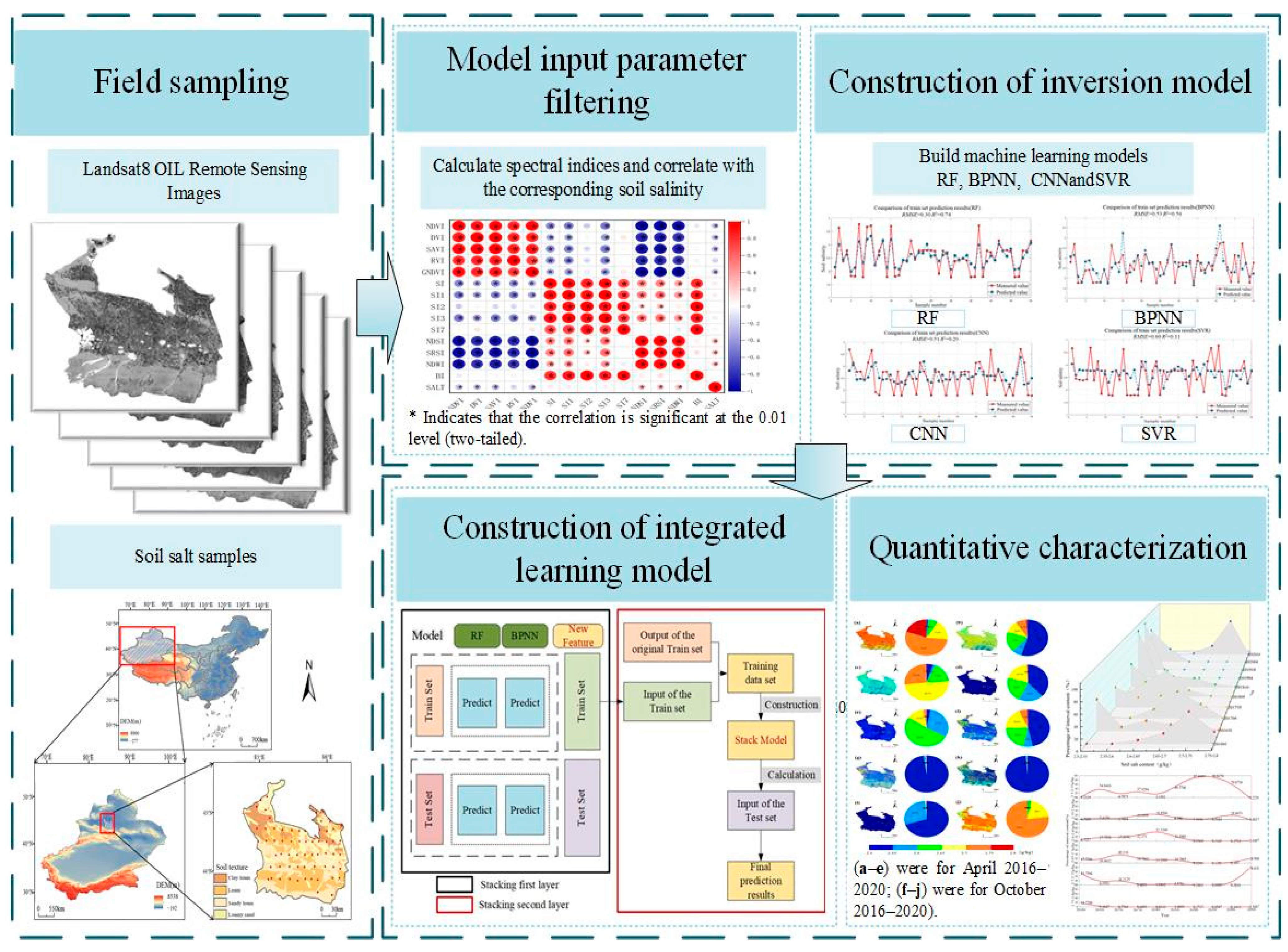
Abstract
Soil salinization is an essential risk factor for agricultural development and food security, and obtaining regional soil salinity information more reliably remains a priority problem to be solved. To improve the accuracy of soil salinity inversion, this study focuses on the Manas River Basin oasis area, the largest oasis farming area in Xinjiang, as the study area and proposes a new soil salinity inversion model based on stacked integrated learning algorithms. Firstly, we selected four machine learning regression models, namely, random forest (RF), back propagation neural network, support vector regression, and convolutional neural network, for performance evaluation. Based on the model performance, we selected the more effective RF and BPNN as the basic regression models and further constructed a stacking integrated learning model. This stacking integration learning model improved the prediction accuracy by training a secondary model to fuse the prediction results of these two basic models as new features. We compared and analyzed the stacking integrated learning model with four single machine learning regression models. Findings indicated that the stacking integrated learning regression model fitted better and had good stability; on the test set, the stacking integrated learning regression model showed a relative increase of 8.2% in R2, a relative decrease of 14.0% in RMSE, and a relative increase of 6.5% in RPD when compared to the RF model, which was the single most effective machine learning regression model, and the stacking model was able to achieve soil salinity inversion more accurately. The soil salinity in the oasis areas of the Manas River Basin tended to decrease from north to south from 2016 to 2020 from a spatial point of view, and it was reduced in April from a temporal point of view. The percentage of pixels with a high soil salinity content of 2.75–2.80 g kg−1 in the study area had decreased by 19.6% in April 2020 compared to April 2016. The innovatively constructed stacking integrated learning regression model improved the accuracy of soil salinity estimation on the basis of the superior results obtained in the training of the single optimal machine learning regression model. As a consequence, this model can provide technological backup for fast monitoring and inversion of soil salinity as well as prevention and containment of salinization.
1. Introduction
Soil salinization is considered to be a significant issue with ecological impacts, strictly proscribing the safety and improvement of regional ecological areas [1,2,3,4]. Cultivated soil salinization is recognized for causing land degradation, harming crop growth, and precluding agricultural improvement [5,6,7,8]. Among them, soil salinization is the most severe in Xinjiang, accounting for 36.8% of the saline soil area in the country. Xinjiang is known as a saline soil museum, which not only has many saline types but also is difficult to manage [9]. As one of the four major agricultural irrigation zones in Xinjiang, the oasis of Manas River Basin, which is affected by water scarcity and salinization of soils, was the first to promote the technology of submerged drip irrigation under the membrane, which has been carried out for more than 20 years now [10]. Therefore, it is of great significance to monitor the salinized soils, in which the under-membrane drip irrigation technology has been implemented for a long time. An ordinary technique for achieving soil salinity statistics has been fixed-point sampling with the use of a conductivity meter to measure the statistics [4,11,12,13,14]. Although this method has been shown to be effective, it has the shortcomings of being time-consuming, labor-intensive, having poor representation of the measurement points, including only a small coverage area, and so forth and has limitations for soil salinity monitoring across large spatial scales [15]. In recent years, as remote sensing technology has been integrated with agriculture, it has been a means of achieving rapid acquisition of records at a lower value [4,16,17,18]. A growing number of remote sensing techniques are being applied to soil salinity monitoring [19,20,21,22]. Feature indices that are more sensitive to salinity are approached from remote sensing images, and a model is structured by incorporating feature indices with soil salinity content to facilitate the monitoring current status of regional soil salinity [8]. This method can make up for the shortcomings of previous field surveys and allow researchers to study regional soil salinization from a larger spatial scale, with the advantages of obtaining information quickly, being less affected by the ground, and being able to continuously and dynamically monitor regional salinization status, making it one of the most widely used quantitative soil salinization monitoring methods today [23].
Inversion of empirical statistical regression models for biophysical parameters of vegetation using remote sensing is usually classified into simply linear regression models, on the one hand, and non-linear regression models, on the other hand. In order to explore the feasibility of using multiple vegetation indexes to invert soil salinity content, Wu et al. [24] estimated soil salinity primarily on the basis of linear regression, synergistic kriging, regression kriging, and geographically weighted regression, and the findings indicated that geographically weighted regression method was the most accurate (RMSE = 0.31), respectively. Although linear regression models could effectively reduce the uncertainty in the inversion process [25], these models are difficult to solve when data are nonlinear or have a high correlation between features. Soil quality prediction methods based on machine learning models have been proposed by many scholars because they do not require knowledge of internal variables and can provide simple solutions for nonlinear and multivariate functions’ [26] reports. Machine learning models have a strong ability to deal with nonlinear relationships between independent and dependent variables, which significantly improves the prediction accuracy and breaks through the limitations of traditional methods [27].
In order to accurately estimate soil water in semiarid areas in the western part of Khorasan-Razavi province in (northeast) Iran, Hamed et al. [28] explored the sensitivity of vegetation indexes calculated from Landsat 8 remote sensing imagery to soil water by using random forest (RF), elastic net regression, and linear regression models, and findings indicated that RF regression model was the most accurate (RMSE = 0.04). Nonlinear regression models can provide an explanation for the correlation between the bio-physical and model variables [29], are easy to parallelize, and have a relatively strong model generalization ability; however, it is often necessary to trade off the balance of such a model with its accuracy if the prediction error of a single regression model is relatively low [30]. Ghosh et al. [31] estimated the biomass of mangrove forests in India making use of a series of machine learning algorithms such as the RF model, gradient boosting model, and extreme gradient boosting model, as well as integration of multiple machine learning algorithms. They found that the accuracy of inverting the aboveground biomass was further improved, showing RMSE to be 72.9 t ha−1, using a stacking algorithm in a multi-temporal image-stacked dataset. This RMSE was 1.6 t ha−1 less than that of the single RF regression model, indicating that an integrated learning regression algorithm based on stacking could integrate multiple underlying regression models and provide enhanced generalization capabilities [32].
Currently, the integrated learning regression model based on stacking has shown good performance in soil water inversion [33,34,35]; however, there is still a need for in-depth research in soil salinity content inversion. Therefore, we attempted to use the stacking integrated learning regression model in soil salinity inversion to obtain more accurate results using the oasis area of the Manas River Basin as a study object.
The study objectives are as follows: (1) to establish soil salinity inversion model with multiple machine learning methods, including random forest (RF) model, back propagation neural network (BPNN) model, support vector regression (SVR) model, convolutional neural network (CNN) model, and stacked integrated learning algorithm; (2) to evaluate and analyze the performance of each model by comparing the prediction accuracies of different machine learning models and evaluating their performances in soil salinity inversion, focusing on the superiority of the stacked integrated learning model among different models; and (3) to quantitatively characterize the spatial and temporal changes of soil salinity in the oasis area of the Manas River Basin, analyze the spatial distribution and temporal dynamic changes of soil salinity content in the area by combining the model prediction results, and provide a detailed description of the regional soil salinity changes to provide technical support and a conceptual foundation for the future use of inversion models.
2. Materials and Methods
2.1. Study Area
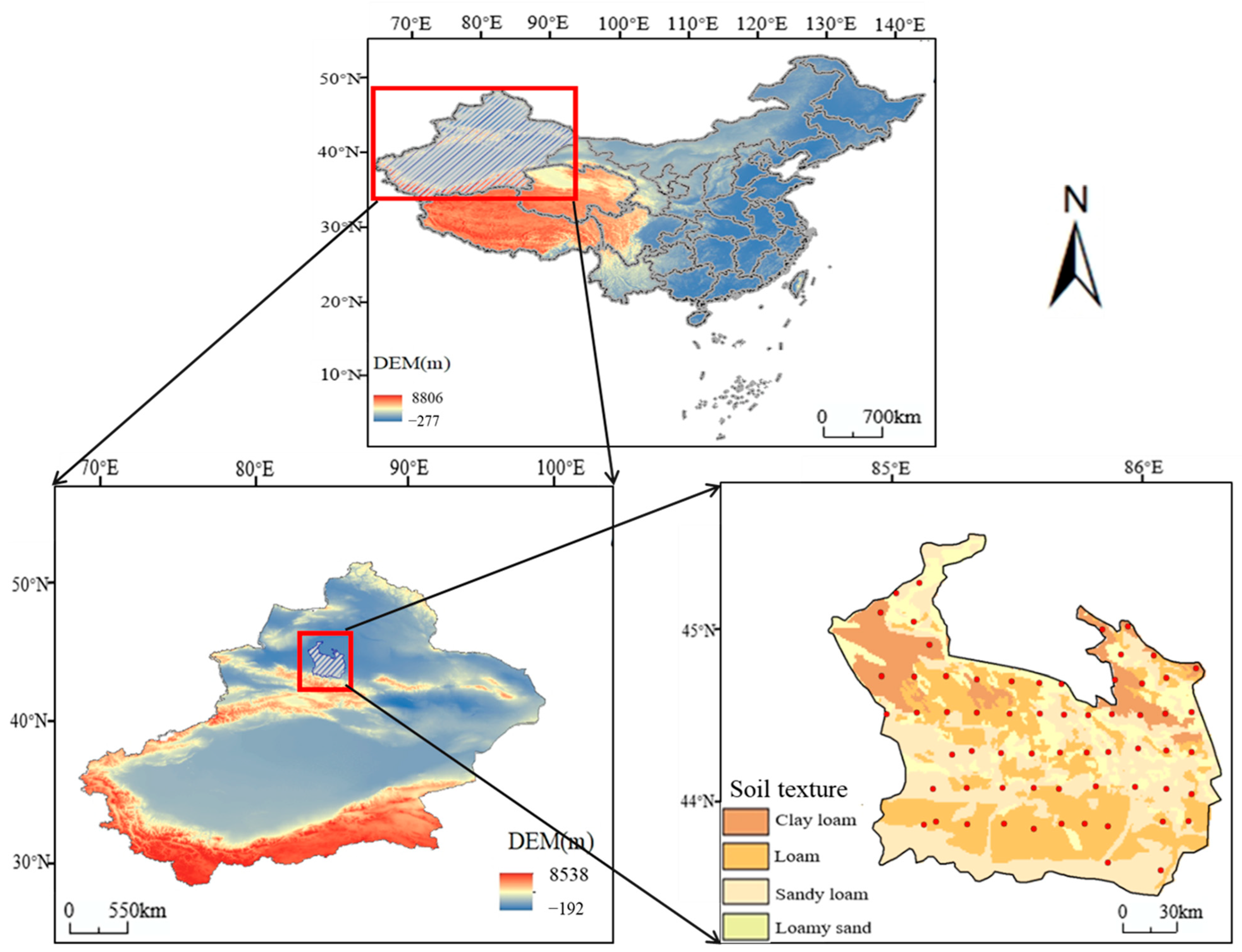
The Manas River Basin Oasis Area lies in the mid-region of the northern foothills of the Tianshan Mountains in China, on the southern edge of the Junggar Basin with a longitude of 85°01′–86°32′ E and a latitude of 43°27′–45°21′ N, as shown in Figure 1. The area includes Lower Nodi Irrigation District, Anzhihai Irrigation District, Jinguhe Irrigation District, Shihezi Irrigation District, Xinhu General Field Irrigation District, and Mosuo Bay Irrigation District [36]. The basin is arid with an average annual temperature of 4.7–5.7 °C, with the highest temperature in July and the lowest in January, an average annual precipitation of 100–200 mm, and, mainly concentrated in summer, an average annual evaporation of 1500–2100 mm [37,38]. Ice and snow meltwater in the region carry salts from rock weathering into farmland. This perennial salt aggregation has resulted in serious salinization of the oasis, and due to the irrationality of irrigation, the salinization of farmland in the Manas River Basin is frequent, seriously affecting the improvement of resource utilization and economic development [39]. Therefore, exploring fashions with greater accuracy is indispensable to understanding regional soil salinity monitoring.
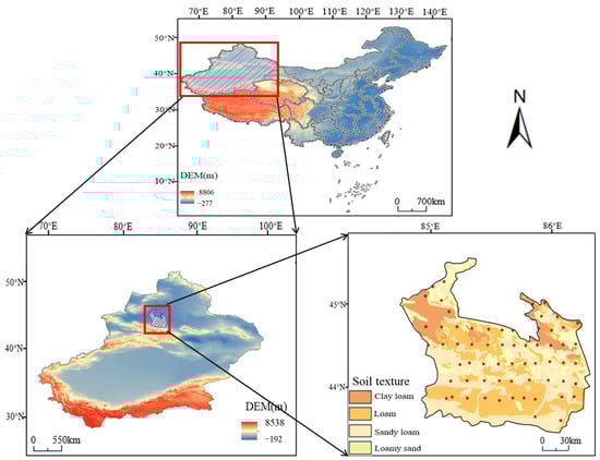
Figure 1.
Distribution of oasis areas and sampling sites in the Manas River Basin (Coordinate system: WGS1984, Datum: WGS84).
2.2. Data Sources
Soil salinity historical data (from April 2014) were sourced from Xin et al. [40]. The boundary information of the oasis area in Manas River Basin was extracted according to the water system map of the Shihezi Reclamation Area of the Bashi Division of Agriculture, and the initial design of field sampling points was combined with the existing research results, taking into account the topographic and geomorphological characteristics of the irrigation area, the soil characteristics and the current state of land use, etc., and the sampling grid with a 10 km spacing was designed. The soil samples were taken with the help of a hand-held GPS in April 2014, and the design of sampling points was adjusted based on the actual conditions of the sampling points, and the actual sampling points are shown in Figure 1. Remote sensing image data were synchronized with surface data, and the data were obtained from Landsat 8 OLI remote sensing image data collected by the United States Geological Survey (accessed on 1 September 2022 at http://glovis.usgs.gov/). The data had been subjected to preprocessing steps such as geometric correction, radiometric correction, FLAASH atmospheric correction, synthesis, and cropping. Moreover, visual interpretation and supervised classification were applied to categorize the land use status to avoid any confusion regarding information about water bodies such as lakes, rivers, ponds, and puddles in the study area during salinity inversion.
2.3. Salinity Index Construction
The spectral index is an easy as well as valid method for measuring characteristic distributions on the land surface. As such, it was already widely used in global and regional land cover monitoring, vegetation classification, and monitoring of environmental change [41,42,43]. In this study, according to the spectral characteristics of the features, we combined the spectral reflectance in various bands into the spectral index and used them as indexes for remote sensing evaluation. Overall, five vegetation indexes, seven salinity indexes, one water index, and one brightness index were selected [5], and their formulas are shown in Table 1. The spectral indices and soil salinity content were analyzed by Origin.

Table 1.
Spectral index and their calculation formula.
2.4. Model Construction and Accuracy Evaluation
2.4.1. Model Construction and Model Parameters Determination
The input and output data of the soil salinity inversion model were soil spectral index values calculated by Landsat 8 and surveyed soil salinity data, respectively, and the model was built by using RF, BPNN, SVR, and CNN models by Matlab 2019.
The grid search method [51] was used to identify the optimal parameters in the machine learning regression model. Certain key parameters greatly affect the behavior and capability of the model.
The number of decision trees in the RF model was set to 200; by setting this value to 200, the model utilizes a sufficient number of trees to ensure that it reduces variance and improves robustness. A higher number of trees typically enhances the model’s ability to generalize but also increases the computational cost; the value of 200 was chosen to strike a balance between computational efficiency and model accuracy; and the minimum samples required for the division of internal nodes was set to 5, this parameter controls the minimum number of samples required to segment internal nodes. Lower values (e.g., 5) allow the model to grow deeper, potentially capturing more complex patterns in the data and thus enhancing the capacity of the model.
The number of iterations of the BPNN model was set to 1500. The number of iterations determines the training time of the model; setting it to 1500 ensures that the neural network has enough training time to minimize the error and converge to the optimal solution. The grid search identifies 1500 as the point at which further iterations will not significantly improve performance, balance efficiency, and accuracy; the error threshold was set to 1 × 10⁻⁵, and the error threshold is a criterion for stopping the training process when the model reaches a sufficient level of accuracy; setting it to 1 × 10⁻⁵ means that the model will stop when the error becomes very small, ensuring a high level of accuracy. The learning rate was set to 0.001, and the learning rate controls how well the model parameters are adjusted relative to the loss gradient; a smaller value like 0.001 ensures that the model is updated gradually, which prevents exceeding the optimal solution.
The number of iterations of the CNN model was set to 1000; as with the BPNN model, the number of iterations for the CNN model controls its training time. A setting of 1000 iterations ensures that the CNN has enough time to learn complex patterns in the data, especially for image-like or spatially related data; the error threshold was set to 1 × 10⁻⁶. This ensures that the CNN stops training only when it reaches a very small error, thus improving accuracy. The learning rate was set to 0.01; a relatively higher learning rate of 0.01 compared to BPNN can help the CNN model converge faster in fewer iterations, CNNs typically have more parameters due to the convolutional layers, and a slightly higher learning rate can help speed up the optimization process.
Finally, the kernel parameter type of the SVR model was set to 0.01, and the kernel parameter controls the impact of individual data points; setting it to 0.01 helps control the model’s flexibility in drawing decision boundaries, a smaller value means that the model is less sensitive to individual points, thus reducing the risk of overfitting in the SVR model. The kernel function of the SVR model was set to “linear”; it is suitable for cases where the data are linearly separable or where the introduction of nonlinearities would not significantly enhance the model performance, and based on the data, a grid search identifies the linear kernel as the best option. The box constraint was set to 1, and the box constraint controls the trade-off between achieving low error in the training data and minimizing model complexity; setting it to 1 ensures that the SVR model is balanced between bias and variance.
The main steps of the stacking integrated learning regression model were as follows: (1) use MATLAB logic statements to optimize the results of the model, which has the best model precision in a single machine learning regression algorithm; (2) randomly select 80% of the data as the training set and the rest as the test set to train the base model and use the trained RF model and BPNN model to predict a training set and a test set; (3) link the training set and the test set to the predicted results of RF and BPNN model to form a new training set and test set; (4) construct a stacking integrated learning regression model; and (5) use the trained integrated model to predict a training set and test set to evaluate the performance of the model.
There are structure and rationale of the stacking integrated learning regression model as shown in Figure 2. The technology roadmap is shown in Figure 3.
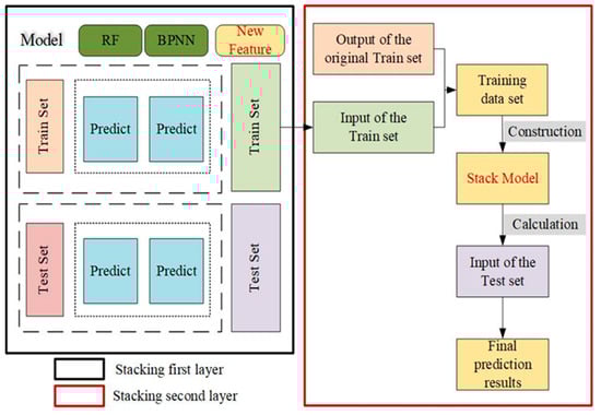
Figure 2.
Principle of the stacking integrated learning regression model.
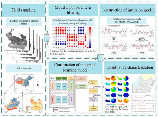
Figure 3.
Research technology roadmap.
2.4.2. Selection of Model Performance Indicators
In this study, the parameters used by Zhao et al. [4] and Peng et al. [5] are used to evaluate model performance: coefficient of determination (R2), RMSE, and relative percentage difference (RPD). Generally, higher R2 values and smaller RMSE values indicate a more favorable model. The RPD was classified into three levels, which were Class A (RPD > 2.0, the constructed model is considered to be highly reliable), Class B (1.40 ≤ RPD ≤ 2.0, the constructed model is considered to be moderately reliable), and Class C (RPD < 1.40, the constructed model is not reliable) [4,5,40]. The formula to calculate the evaluation indicators is as follows:
where , , and are the predicted, measured, and average measured values of soil salinity, respectively, and n is the number of samples.
3. Results
3.1. Correlation Analysis between Spectral Indexes and Soil Salinity
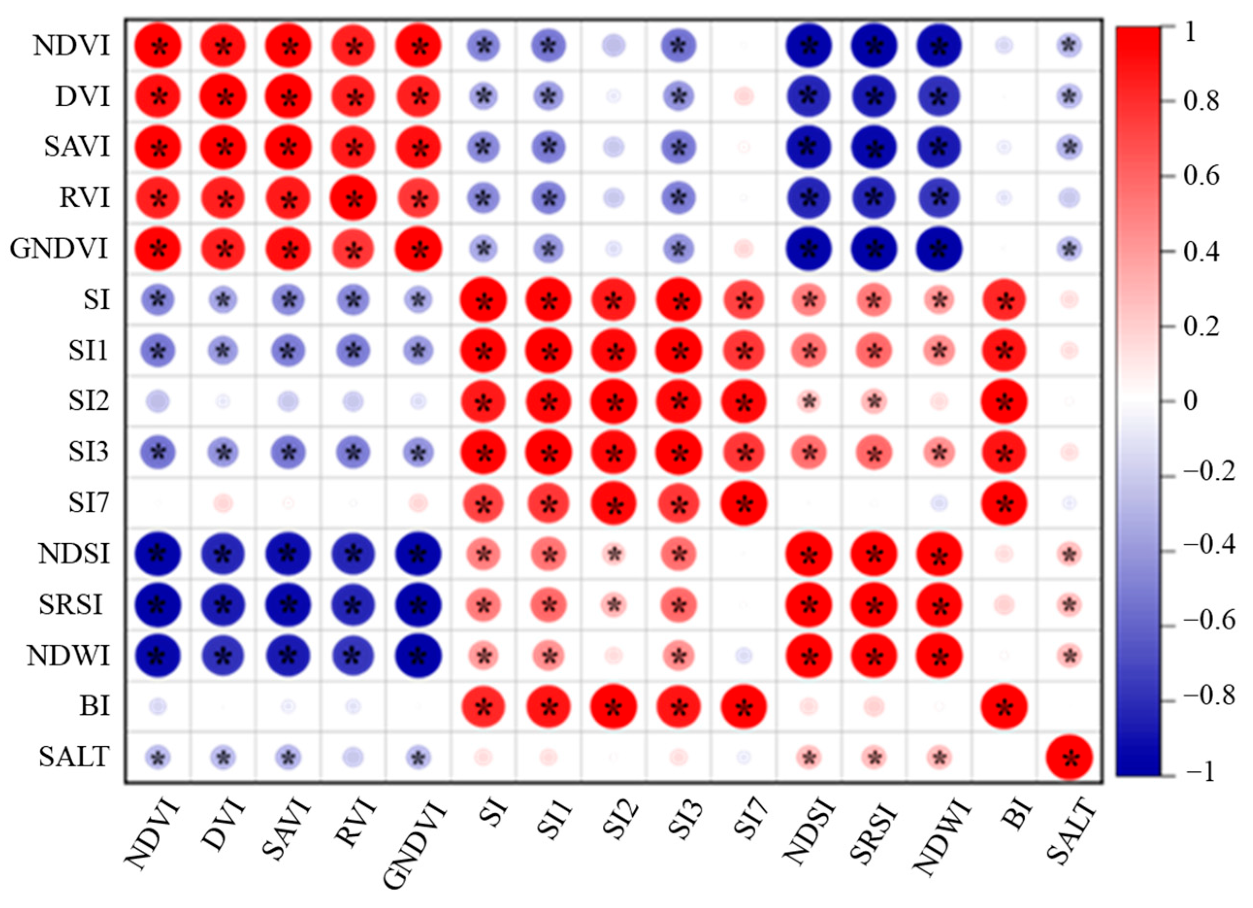
There were 14 soil spectral indicators and soil salinity derived from Origin 2018 software, which conformed to the normal distribution test; the results of Pearson correlation analysis are shown in Figure 4.

Figure 4.
Correlation between spectral index and soil salinity. Note: * Indicates that the correlation is significant at the 0.01 level (two-tailed).
As seen in Figure 4, among the triangular vegetation index, salinity index, water index, and brightness index, only the brightness index has no significant correlation with soil salinity, indicating that the relationship between soil salinity and the brightness index is relatively weak. Normalized Difference Snow Index (NDSI) and Standardized Reservoir Supply Index (SRSI) are positively correlated with soil salinity, and these indexes have large values in high salinity areas, reflecting the accumulation of soil salinity. Normalized Difference Water Index (NDWI) also shows a positive correlation with soil salinity. The Normalized Difference Vegetation Index (NDVI), Difference Vegetation Index (DVI), Soil-Adjusted Vegetation Index (SAVI), and Green Normalized Difference Vegetation Index (GNDVI) are negatively correlated with soil salinity, which indicates that in areas of high salinity, the growth and cover of vegetation was poorer and high salinity inhibited the normal growth of plants, resulting in a negative correlation.
3.2. Evaluation of Machine Learning Regression Models
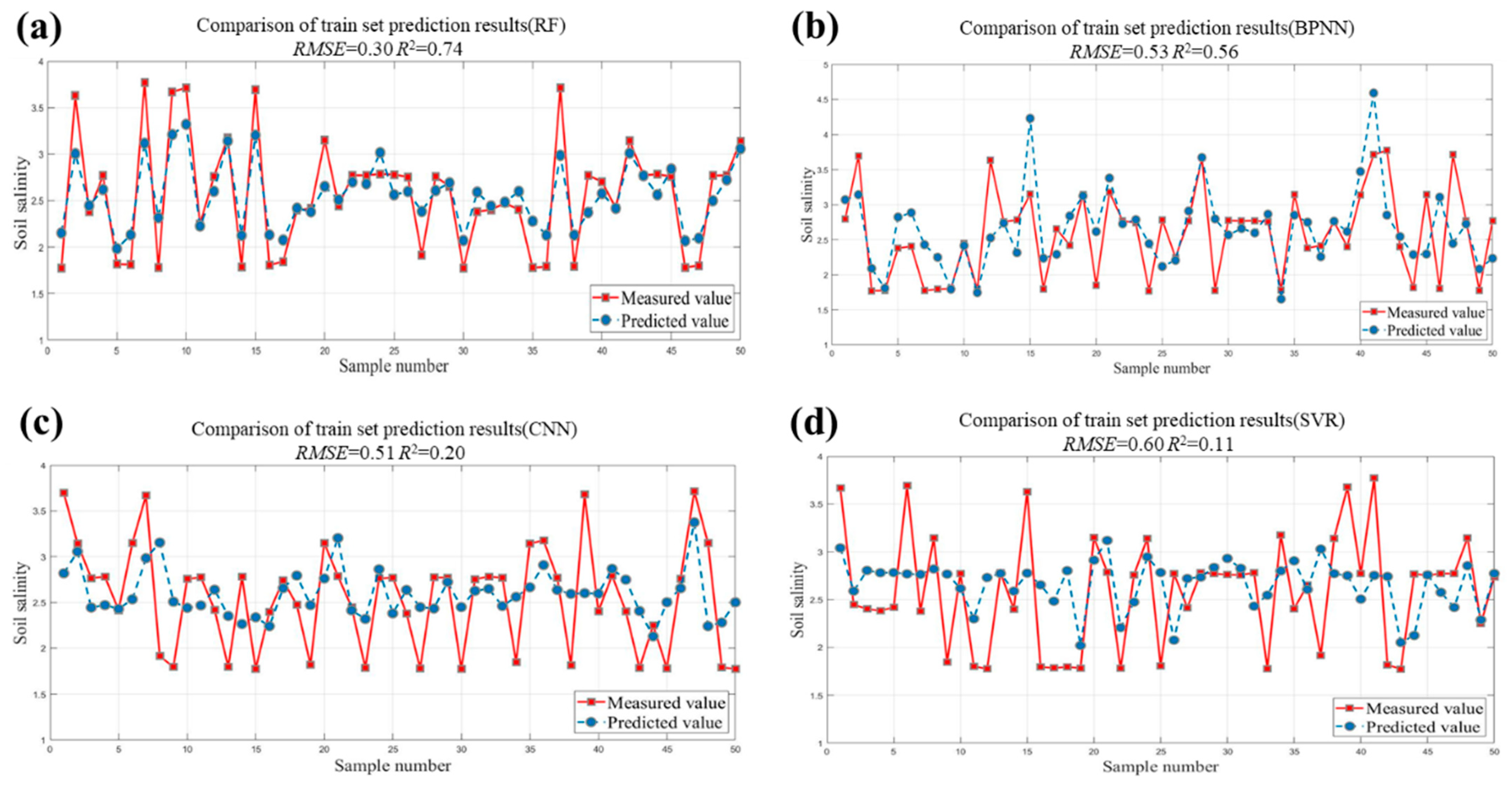
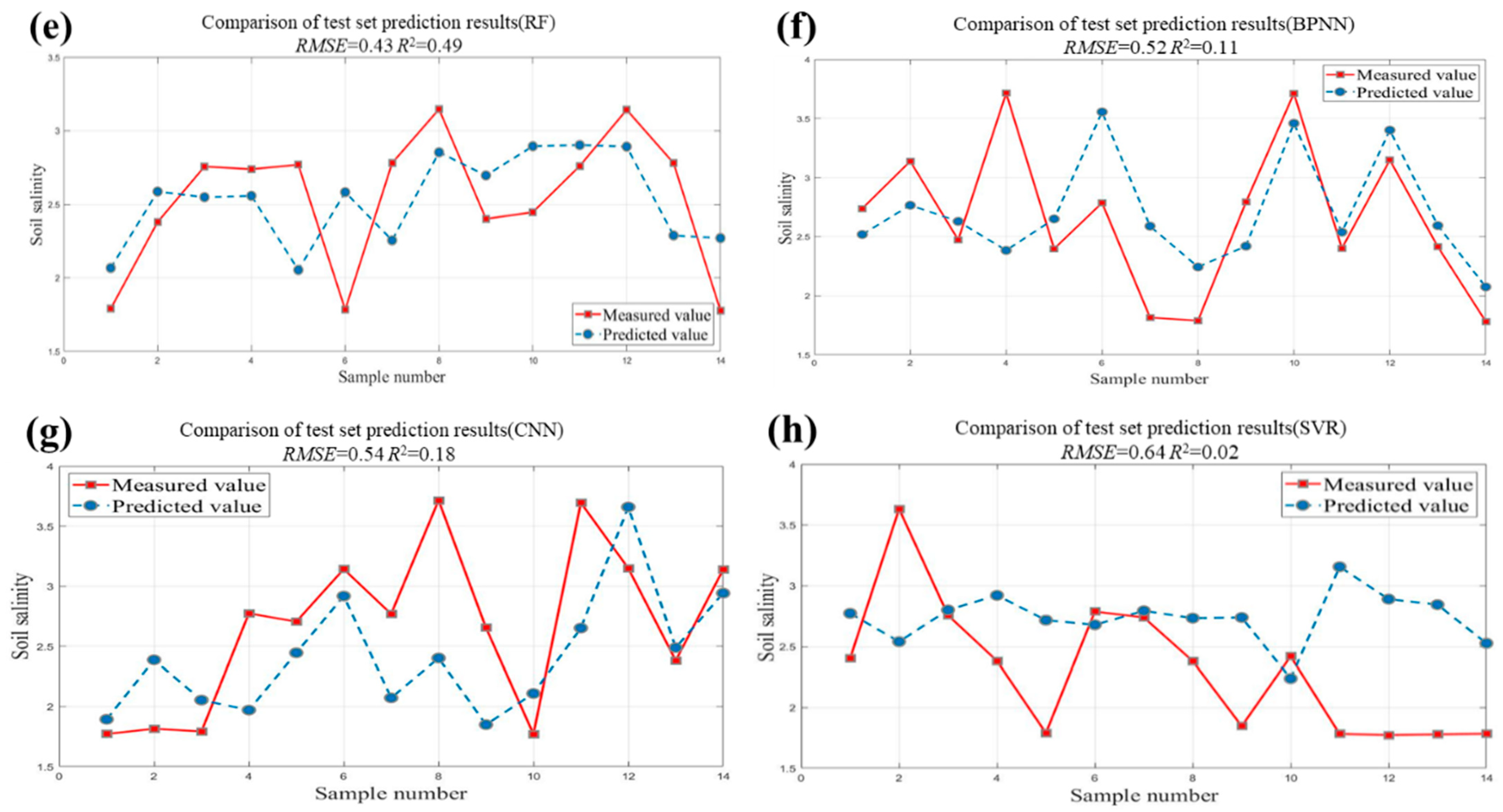
The spectral index data (NDSI, SRSI, NDWI, NDVI, DVI, SAVI, and GNDVI) with good correlation and the corresponding soil salinity data were used as the input data of models. Four machine learning methods (RF, BPNN, CNN, and SVR) were used to construct the soil salinity inversion models; prediction results are shown in Table 2. Forecast values of four inversion models of soil salinity had been in comparison against the measurements of soil salinity, as shown in Figure 4.
Table 2.
Inversion model results of soil salinity based on spectral indices.
As seen in Table 2 and Figure 5, the single optimal machine learning regression model was the RF. On the training set, both the RF and BPNN achieved better inversion results with R2 above 0.50, RMSEs of 0.30 and 0.53, respectively, and RPDs of 1.4 or more, which reflects high accuracy. Meanwhile, the CNN and SVR models underperform poorly on the training set, with R2 of 0.20 and 0.11, RMSEs of 0.51 and 0.60, and RPDs below 1.4, respectively, indicating that the constructed models were unreliable. On the test set, the best inversion model was RF which had R2 of 0.49, RMSE of 0.43, and RPD of 1.40, with accuracies 23%, 31%, and 47% higher than those of the BPNN, CNN, and SVR models, respectively; the R2 of the four models, in descending order, was RF > BPNN > CNN > SVR, and the RMSEs were the opposite of this. According to the model performance evaluation index, it was reasonable to use the spectral index to establish the model. Therefore, in this paper, the RF and BPNN models with better inversion results were selected as the base models for the stacking integrated learning regression.
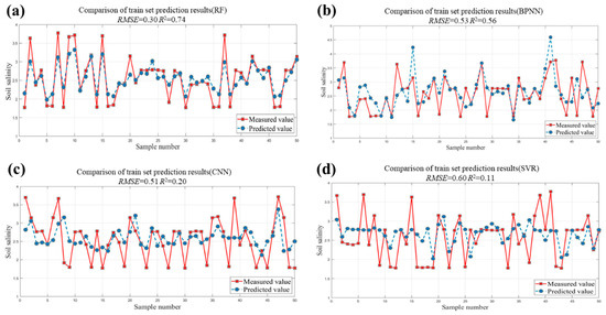
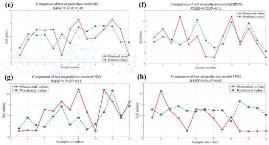
Figure 5.
Prediction results for RF, BPNN, CNN, and SVR ((a–d) are the prediction results for the RF, BPNN, CNN, and SVR training set and (e–h) are the prediction results for the RF, BPNN, CNN, and SVR test set, respectively).
3.3. Stacking Integrated Learning Regression Model Evaluation
The stacking integrated learning regression model can integrate many basic regression models and so forth to create much stronger predictions and deliver enhanced capabilities of generalization during inversion. The prediction results of the training set and test set of the stacking integrated learning regression model are shown in Figure 6.
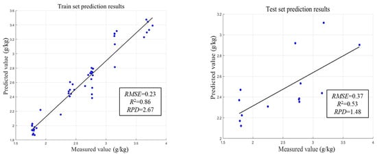
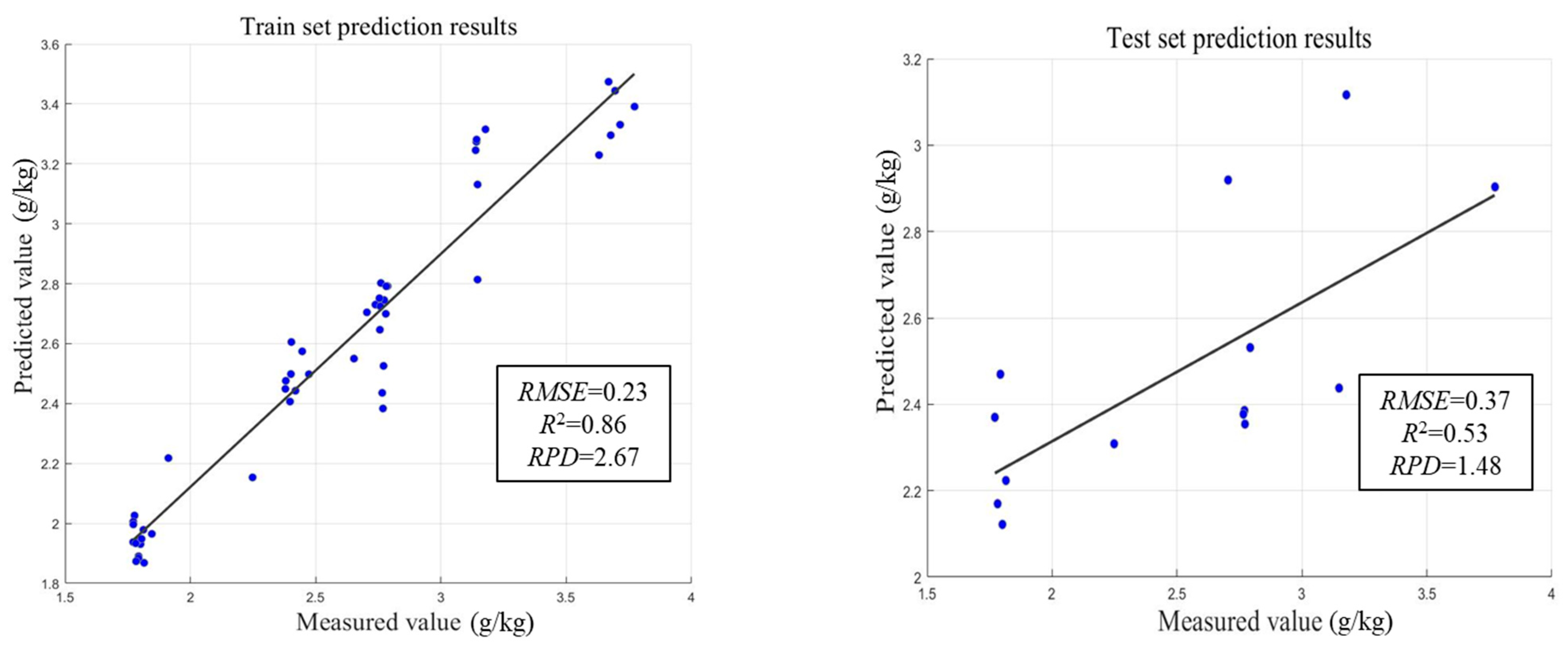
Figure 6.
Scatter plot of measured and predicted values of a stacking integrated learning regression model.
As seen in Figure 6, the stacking integrated learning regression model has high integration capability, and the model fit is strong as derived from the fitting curves. On the training set, the R2 was 0.86, the RMSE was 0.23, and the RPD was 2.67, and on the test set, the R2 was 0.53, the RMSE was 0.37, and the RPD was 1.48, which shows that the model has good stability.
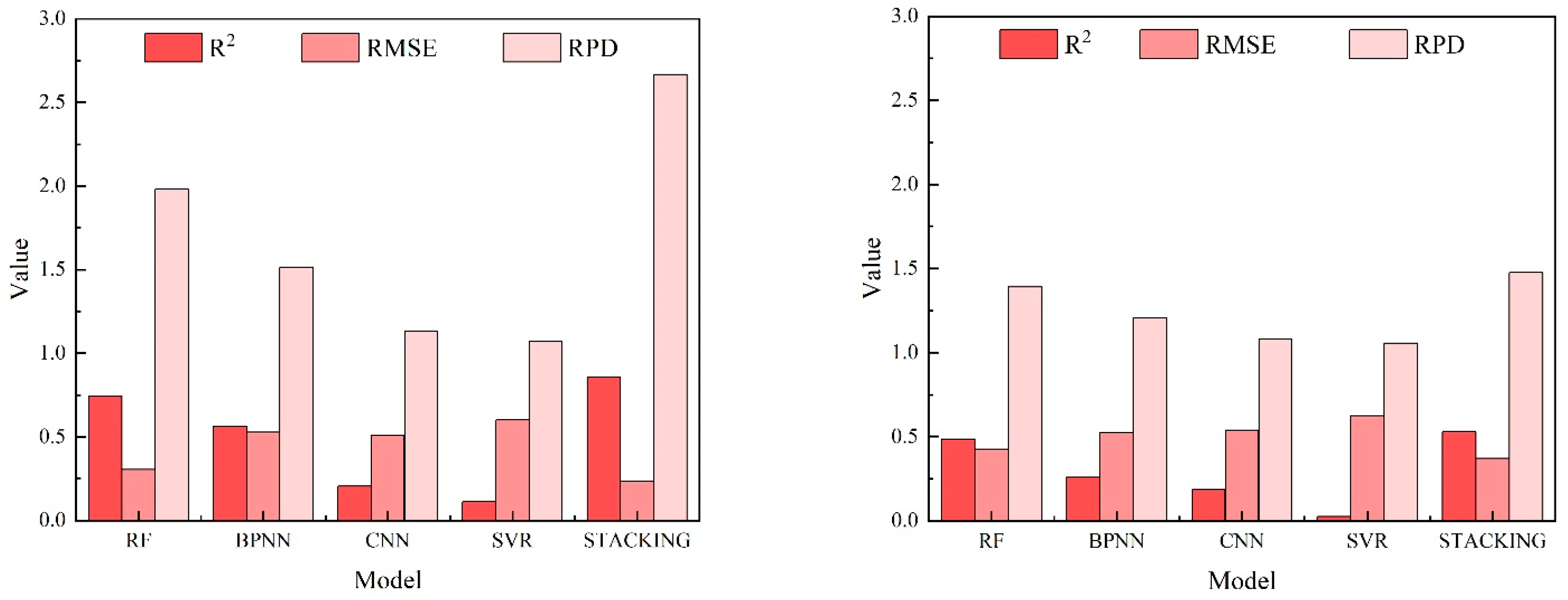
A performance comparison of the results of stacking integrated learning, RF, BPNN, CNN, and SVR regression models is shown in Figure 7. As seen in Figure 6, on the training set, the R2 of the stacking integrated learning regression model relatively improved by 16.2%, the RMSE relatively reduced by 23.3%, the RPD relatively improved by 34.9% compared with the single optimal RF model, which changed from being a moderately reliable model to a model with higher reliability that can be used for model analysis. On the test set, the R2 of the stacking integrated learning regression model was relatively improved by 8.2%, the RMSE was relatively reduced by 14.0%, and the RPD was relatively improved by 6.5% compared with the RF. In summary, the integrated learning regression model had a stronger generalization ability and improved the estimation accuracy of soil salinity once again on the basis of the superior results obtained in the training of the single optimal machine learning regression model.

Figure 7.
Performance evaluation of stacking integrated learning, RF, BPNN, CNN, and SVR regression models. Note: The left figure is the training set and the right figure is the test set.
3.4. Spatiotemporal Distribution of Soil Salinity
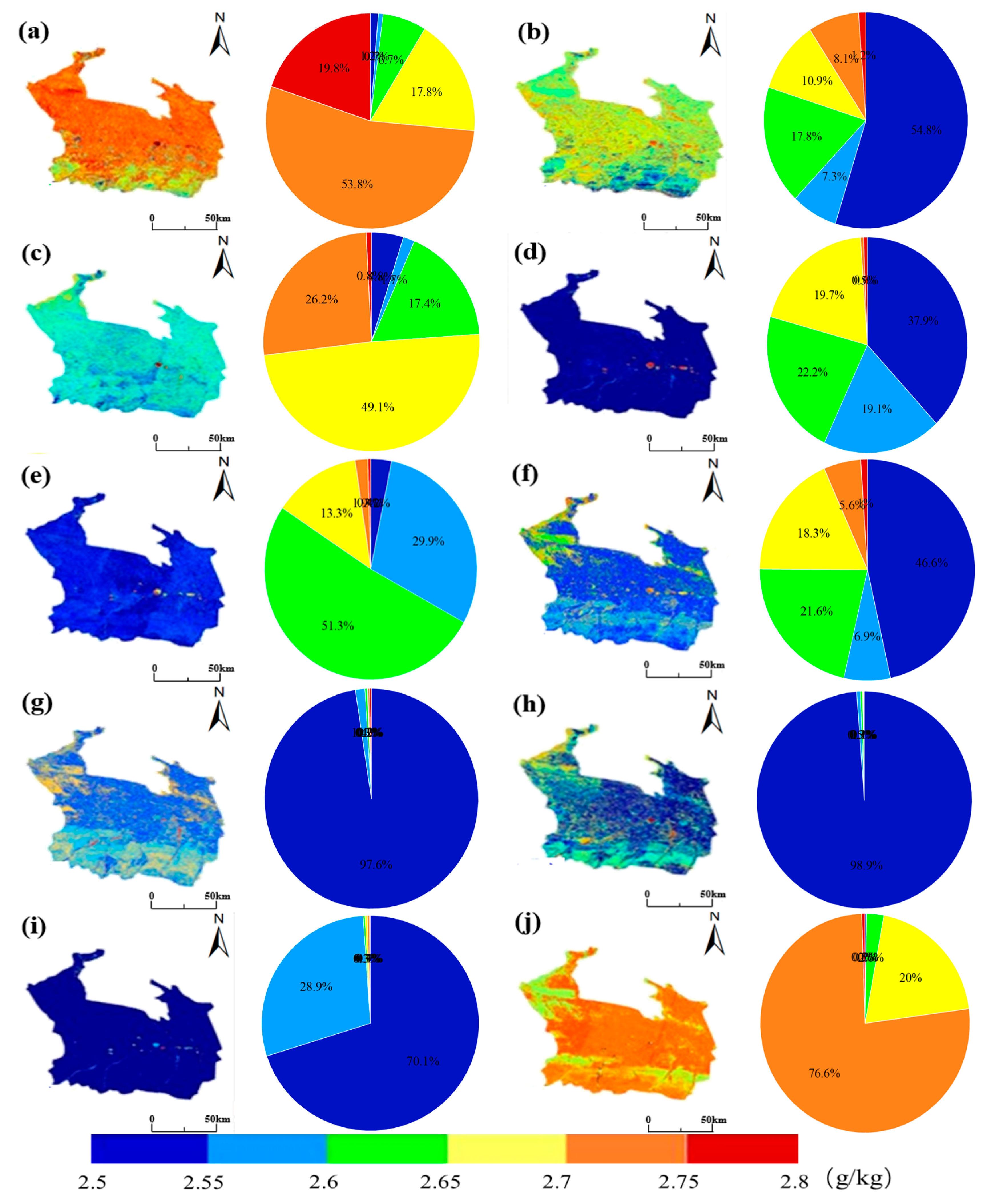
To better reflect the inversion effect of the model, the spatial distribution of soil salinity in the study area in April and October 2016–2020 was mapped based on the constructed stacking integrated learning regression model. As seen in Figure 8, there was a significant difference in soil salinity. From a spatial point of view, the soil salinity content in the study area in April and October of 2016, 2017, and 2018 showed a decreasing trend from north to south, with more pronounced salinization in the east-central part (near the Manas power plant and the town of Anjihai). In 2016, 2017, and 2018, the average salt content in April was 2.71, 2.67, and 2.61 g kg−1, respectively, and the average salt content in October was 2.53, 2.57, and 2.58 g kg−1, respectively. The values from October were lower by 0.18, 0.10, and 0.03 g kg−1, respectively, compared to April. There was no significant change in soil salinity in most areas in April and October 2019. The average value of soil salinity in October 2020 was 2.71 g kg−1, which was significantly higher, by 7.2%, compared to that of April of the same year.

Figure 8.
Spatial distribution of soil salinity in April and October 2016–2020 ((a–e) were for April 2016–2020; (f–j) were for October 2016–2020). Note: Pie charts were regional shares of salinity content.
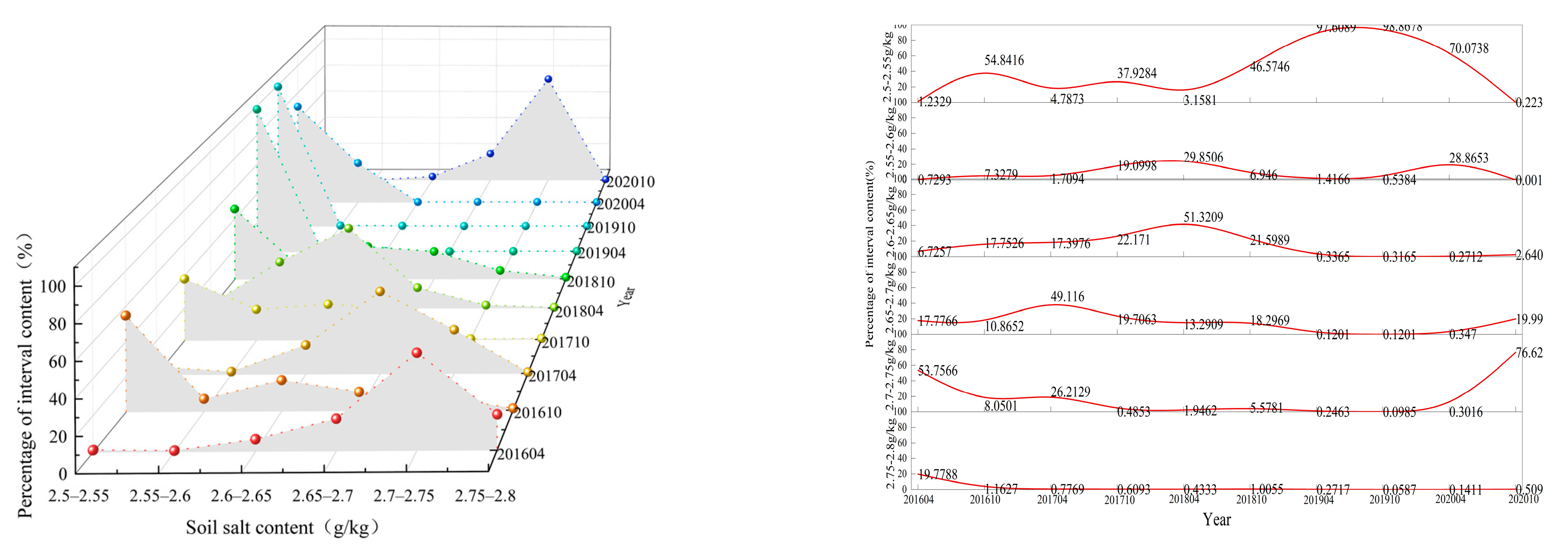
As can be seen from Figure 9, the percentage of pixels with high soil salinity content of 2.75–2.80 g kg−1 in the study area in April 2016, October 2016, April 2020, and October 2020 was 19.8%, 1.2%, 0.1%, and 0.5%, respectively. These values decreased by 19.6% in April 2020 compared to April 2016, indicating a reduction in salinization. From 2016 to 2018, 55.3% of the area’s soil salinity shifted from 2.65–2.80 g kg−1 to 2.50–2.65 g kg−1, especially from October to April. Soil salinity was maintained at 2.50–2.55 g kg−1 in 70.1% of the area in 2019. However, soil salinity intensified in October compared to April 2020, with 96.3% of the area shifting from 2.55–2.65 g kg−1 to 2.65–2.80 g kg−1, probably due to the disturbance of vegetation cover when acquiring remote sensing images. Overall, in April, the degree of soil salinization in the oasis area of the Manas River Basin decreased gradually, and the saline–alkaline land improvement measures were still effective.
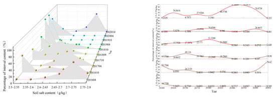
Figure 9.
Soil salinity content over time.
4. Discussion
Accurately monitoring soil salinity content is essential for both food production and precision agriculture construction [52]. In this paper, a Pearson correlation analysis was introduced to filter the characteristics in spectral indices [53], and the findings of this study indicated that the dominant factors of soil salinity were mainly vegetation index, salinity index, and water index, and this is in agreement to Alhammadi et al. [45,46,47,48]. The difference was that this study obtained a significant correlation between water index and soil salinity. Soil salinity migrates as soil moisture moves, and there will be an increase in soil electrical conductivity and higher soil moisture content in areas with higher soil salinity [54,55]. Tang et al. [56] also find that the albedo of salinized soil increases due to the specular effect of water bodies as soil moisture content increases towards a critical point. Therefore, the water index, vegetation index, and salinity index were input as variables for the building of soil salinity inversion models.
The development of machine learning algorithms has accelerated the remote sensing modeling process. Many machine learning algorithms often exceed the accuracy of traditional regression modeling [44,45,46]. In this research, four machine learning regression models, RF, BPNN, CNN, and SVR, had been made to simulate soil salinity, and their parameters (e.g., number of decision trees, depth, and regularization coefficients) directly affect the performance of the models. Without optimization, the performance of individual models may fluctuate, and optimizing these hyper-parameters through grid search methods can lead to better performance. RF obtained the best inversion results with R2 of 0.74, RMSE of 0.30, and RPD of 1.98. Wei et al. [57] quantitatively estimated soil salinity by using multispectral imagery from unmanned aerial vehicles and established the BPNN, SVR, and RF models, and their findings indicated that the RF model was the most effective. Zhang et al. [58] explored the problem of rapid monitoring of soil salinity. They used support vector machine, BPNN, RF, and multivariate linear regression models to establish soil salinity, and their findings indicated that the RF model is optimal with an R2 of 0.72; this is in agreement well with this research.
Because of both plant individual differences and changes in canopy over the seasons, there is often a shortcoming of a single machine learning model with poor generalizations [8]. Yang et al. [8,59] presented a stacking approach to accomplish the task of efficiently estimating highly accurate forecasts by combining a number of weak forecasters into one powerful forecaster, which can effectively improve estimation accuracy. Presently, while integrated learning models on the basis of stacking algorithms are broadly applied for the domains of machine vision and natural language processing, the application of integrated learning models for soil salinity has not been explored in terms of stacking strategy [8]. In this study, we constructed a stacking-based integrated regression model which has the advantage of combining the prediction results of multiple models, reducing the over-reliance on the parameterization of a single model, and having better robustness and generalization capabilities, thus improving the overall accuracy and stability, with an R2 increase more than 16.2% compared to a single machine learning regression model based on a training set. Thus, there is a significant advantage of the stacking algorithm in predicting soil salinity. In other words, the more complex integration algorithm, that is, the stacking integration model, is significantly more capable of handling complex problems than the single machine learning regression model, a finding also supported by Pham et al. [60]. The first layer of the stacking method consists of various underlying models with inputs from the original training set, while the outputs are the predicted values of the various base models. The second layer consists of only one meta-model, which is trained on the forecast and true values of the various models in the first layer to form a completely integrated model. Similarly, the process of predicting the test set goes through the predictions of all the base models to compose the features of the second layer; next, a second layer of the meta-model is implemented to predict final outputs in order to keep approaching the true value [61], which could be prone to overfitting if the training set of the base models is used directly to generate the training set of the meta-model. This study focused on RF- and BPNN-based models rather than those based on CNN and SVR. This was because the RF- and BPNN-based models obtained better results than the CNN- and SVR-based models when we tested the model performance. However, although the stacked integration model can provide higher prediction accuracy, its internal mechanism is more complex and it is difficult to intuitively explain the contribution of each input variable to the output results. In practice, this “black box” effect may cause confusion for decision-makers, and it is also dependent on the amount of data and may suffer from overfitting problems when the amount of data is small; the approach to combining the advantages of a single model to build an integrated model remains the key to future research.
The stacking integrated learning regression model was constructed to carry out soil salinity inversion with the oasis zone of the Manas River Basin as the research object. Findings of research show that soil salinity content in this area had a decreasing trend from north to south in 2016, 2017, and 2018. The region of study is a typical mountain-basin structural system and sees differences in soils, water table, and climate based on latitude and location [62]. Zhang et al. found that a low-latitude area had a long development time, high soil maturity, and low soil salinity. Meanwhile, a mid-latitude area had a high water table, and with the promotion of membrane drip irrigation technology, the crop area could expand rapidly. Moreover, the membrane drip irrigation technology did not remove the salinity, so the mid-latitude area had a higher soil salinity. Finally, a high-latitude area that situated at the lower river basin and had a texture that was dominated by sandy loam and sandy soil would have a low water table. The soil salinity would also be higher than that in the mid-latitude area [63,64,65]; this is in agreement with this study’s results. In 2016–2018, soil salinity was reduced in October compared with April, probably because the change in groundwater burial depth during the year showed a mining type. Then in October, the groundwater declined rapidly, and the deeper groundwater burial depth and frequent agricultural irrigation made soil salinity decrease in the month. This is in accordance with the findings of Chen et al. [66] on soil salinity and nutrients in different landscape types. However, in April and October 2019, there was no significant change in soil salinity in the vast majority of the area. Soil salinity became stronger in 2020 compared to 2019, especially in October 2020, when soil salinity increased significantly. As temperatures increased, soil water rose vigorously, and salts then increased and accumulated on the soil surface. This has been similar to Zhao et al.’s [67] study on 121 Corps, 8th Agricultural Division, Manas River Basin, where crop soil salinity showed a salt accumulation trend in early May and mid-September. The integrated learning regression model constructed in this study is a fast and accurate inversion of soil salinity content for quantitative assessment and monitoring of saline soils regionally. However, there are some common limitations of satellite data (e.g., Landsat 8 OLI) for soil salinity inversion: The low spatial and temporal resolution may not be sufficient for fine-scale, high-precision monitoring, and different types of surface (e.g., vegetation, water) affect the spectral reflectance of the soil, which can interfere with the accuracy of the inversion model. If the ground data are insufficient or unevenly distributed, the accuracy of the model and the reliability of the results may be affected. Therefore, there may be significant differences in soil salinity distribution patterns for refined cropping structures, which need to be further investigated in the future.
5. Conclusions
We constructed soil salinity inversion models by combining Landsat 8 OLI remote sensing data and four methods of machine learning. Findings indicated that the single optimal machine learning regression model was the RF. In addition, the innovative stacking integrated learning regression model that was constructed in this study yielded better soil salinity inversion results, with a relative increase of 16.2% in the R2, a relative decrease of 23.3% in the RMSE, and a relative increase of 34.9% in the RPD on the training set compared with the single optimal machine learning regression model. On the test set, the R2 was relatively improved by 8.2%, the RMSE was relatively reduced by 14.0%, and the RPD was relatively improved by 6.5%. Soil salinity in the oasis area of the Manas River Basin was accurately predicted and characterized. The soil salinity content in this area in April and October of 2016, 2017, and 2018 shows a trend of decreasing from north to south. And it gradually decreased in April, with the percentage of pixels with high soil salinity content of 2.75–2.80 g kg−1 in the study area decreasing by 19.64% in April 2020 compared to April 2016. Overall, the regression model on the basis of stacking had high accuracy, which could be of important relevance toward the quick abstraction of salinity status and soil salinity maintenance and management in the Manas River Basin. However, further exploration is needed to combine the advantages of multiple single models to construct an integrated model, and this consideration is the key to future research.
Author Contributions
Conceptualization, H.D. and F.T.; methodology, H.D. and F.T.; software, H.D.; validation, H.D. and F.T.; formal analysis, H.D.; investigation, H.D.; resources, F.T.; data curation, H.D.; writing—original draft preparation, H.D.; writing—review and editing, H.D. and F.T.; visualization, H.D.; supervision, F.T.; project administration, F.T.; funding acquisition, F.T. All authors have read and agreed to the published version of the manuscript.
Funding
This research was funded by the National Key Research and Development Program of China (2021YFD1900800), the National Natural Science Foundation of China (52179049) and the Western Light-Key Laboratory Cooperative Research Cross-Team Project of the Chinese Academy of Sciences (xbzg-zdsys-202103).
Institutional Review Board Statement
Not applicable.
Data Availability Statement
The data presented in this study are available on request from the corresponding author.
Conflicts of Interest
The authors declare no conflicts of interest.
References
- Ivushkin, K.; Bartholomeus, H.; Bregt, A.K.; Pulatov, A.; Sousa, L.D. Global mapping of soil salinity change. Remote Sens. Environ. 2019, 231, 111260. [Google Scholar] [CrossRef]
- Allbed, A.; Kumar, L.; Aldakheel, Y.Y. Assessing soil salinity using soil salinity and vegetation indices derived from IKONOS high-spatial resolution imageries: Applications in a date palm dominated region. Geoderma 2014, 230–231, 1–8. [Google Scholar] [CrossRef]
- Metternicht, G.I.; Zinck, J.A. Remote sensing of soil salinity: Potentials and constraints. Remote Sens. Environ. 2003, 85, 1–20. [Google Scholar] [CrossRef]
- Zhao, W.; Zhou, C.; Zhou, C.; Ma, H.; Wang, Z. Soil Salinity Inversion Model of Oasis in Arid Area Based on UAV Multispectral Remote Sensing. Remote Sens. 2022, 14, 1804. [Google Scholar] [CrossRef]
- Peng, J.; Biswas, A.; Jiang, Q.; Zhao, R.; Hu, J.; Hu, B.; Shi, Z. Estimating soil salinity from remote sensing and terrain data in southern Xinjiang Province, China. Geoderma 2019, 337, 1309–1319. [Google Scholar] [CrossRef]
- Wang, Z.; Zhang, X.; Zhang, F.; Weng, N.; Liu, S.; Deng, L. Estimation of soil salt content using machine learning techniques based on remote-sensing fractional derivatives, a case study in the Ebinur Lake Wetland National Nature Reserve, Northwest China. Ecol. Indic. 2020, 119, 106869. [Google Scholar] [CrossRef]
- Wang, S.; Chen, Y.; Wang, M.; Zhao, Y.; Li, J. SPA-Based Methods for the Quantitative Estimation of the Soil Salt Content in Saline-Alkali Land from Field Spectroscopy Data: A Case Study from the Yellow River Irrigation Regions. Remote Sens. 2019, 11, 967. [Google Scholar] [CrossRef]
- Ding, Y.; Zhang, J. Estimation of SPAD value in tomato leaves by multispectral images. J. Phys. Conf. Ser. 2020, 1634, 012128. [Google Scholar] [CrossRef]
- Zheng, M.; Bai, Y.; Zhang, J.; Ding, B.; Xiao, J. Characterization of soil salinity in typical oasis soils in arid zones based on principal component analysis--taking the 31st regiment of the second division of Xinjiang as an example Shan. Chin. Agron. Bull. 2020, 36, 81–87. [Google Scholar]
- Li, W.; Wang, Z.; Zhang, J.; Zong, R. Soil salinity variations and cotton growth under long-term mulched drip irrigation in saline alkali land of arid oasis. Irrig. Sci. 2022, 40, 103–113. [Google Scholar] [CrossRef]
- Narjary, B.; Meena, M.D.; Kumar, S.; Kamra, S.K.; Sharma, D.K.; Triantafilis, J. Digital mapping of soil salinity at various depths using an EM38. Soil Use Manag. 2018, 35, 232–244. [Google Scholar] [CrossRef]
- Csillag, F.; Pásztor, L.; Biehl, L.L. Spectral band selection for the charac-terization of salinity status of soils. Remote Sens. Environ. 1993, 43, 231–242. [Google Scholar] [CrossRef]
- Eldeiry, A.A.; Garcia, L.A. Detecting Soil Salinity in Alfalfa Fields using Spatial Modeling and Remote Sensing. Soil Sci. Soc. Am. J. 2008, 72, 201–211. [Google Scholar] [CrossRef]
- Kalra, N.K.; Joshi, D.C. Potentiality of Landsat, SPOT and IRS satellite imagery, for recognition of salt affected soils in Indian Arid Zone. Int. J. Remote Sens. 1996, 17, 3001–3014. [Google Scholar] [CrossRef]
- Ding, J.; Yu, D. Monitoring and evaluating spatial variability of soil salinity in dry and wet seasons in the Werigan–Kuqa Oasis, China, using remote sensing and electromagnetic induction instruments. Geoderma 2014, 235–236, 316–322. [Google Scholar] [CrossRef]
- Ma, Y.; Chen, H.; Zhao, G.; Wang, Z.; Wang, D. Spectral Index Fusion for Salinized Soil Salinity Inversion Using Sentinel-2A and UAV Images in a Coastal Area. IEEE Access 2020, 8, 159595–159608. [Google Scholar] [CrossRef]
- Bannari, A.; El-Battay, A.; Bannari, R.; Rhinane, H. Sentinel-MSI VNIR and SWIR Bands Sensitivity Analysis for Soil Salinity Discrimination in an Arid Landscape. Remote Sens. 2018, 10, 855. [Google Scholar] [CrossRef]
- Dehni, A.; Lounis, M. Remote Sensing Techniques for Salt Affected Soil Mapping: Application to the Oran Region of Algeria. Procedia Eng. 2012, 33, 188–198. [Google Scholar] [CrossRef]
- Aldabaa, A.A.A.; Weindorf, D.C.; Chakraborty, S.; Sharma, A.; Li, B. Combination of proximal and remote sensing methods for rapid soil salinity quantification. Geoderma 2015, 239–240, 34–46. [Google Scholar] [CrossRef]
- Li, Y.; Wang, C.; Wright, A.; Liu, H.; Zhang, H.; Zong, Y. Combination of GF-2 high spatial resolution imagery and land surface factors for predicting soil salinity of muddy coasts. CATENA 2021, 202, 105304. [Google Scholar] [CrossRef]
- Xu, Y.; Smith, S.E.; Grunwald, S.; Abd-Elrahman, A.; Wani, S.P.; Nair, V.D. Estimating soil total nitrogen in smallholder farm settings using remote sensing spectral indices and regression kriging. CATENA 2018, 163, 111–122. [Google Scholar] [CrossRef]
- An, D.; Zhao, G.; Chang, C.; Wang, Z.; Li, P.; Zhang, T.; Jia, J. Hyperspectral field estimation and remote-sensing inversion of salt content in coastal saline soils of the Yellow River Delta. Int. J. Remote Sens. 2016, 37, 455–470. [Google Scholar] [CrossRef]
- Qiu, Y.; Chen, C.; Han, J.; Wang, X.; Wei, S.; Zhang, Z. Satellite remote sensing estimation modeling of soil salinity in the irrigation domain of Jiefangzha under vegetation cover conditions. Water Sav. Irrig. 2019, 10, 108–112. [Google Scholar]
- Wu, C.; Liu, G.; Huang, C. Prediction of soil salinity in the Yellow River Delta using geographically weighted regression. Arch. Agron. Soil Sci. 2017, 63, 928–941. [Google Scholar] [CrossRef]
- Lin, C.Y.; Lin, C. Using Ridge Regression Method to Reduce Estimation Uncertainty in Chlorophyll Models Based on Worldview Multispectral Data. In Proceedings of the IGARSS 2019—2019 IEEE International Geoscience and Remote Sensing Symposium, Yokohama, Japan, 28 July–2 August 2019; pp. 1777–1780. [Google Scholar]
- Wu, L.; Peng, Y.; Fan, J.; Wang, Y.; Huang, G. A novel kernel extreme learning machine model coupled with K-means clustering and firefly algorithm for estimating monthly reference evapotran-spiration in parallel computation. Agric. Water Manag. 2021, 245, 106624. [Google Scholar] [CrossRef]
- Xiao, C.; Ji, Q.; Chen, J.; Zhang, F.; Li, Y.; Fan, J.; Wang, H. Prediction of soil salinity parameters using machine learning models in an arid region of northwest China. Comput. Electron. Agric. 2023, 204, 107512. [Google Scholar] [CrossRef]
- Adab, H.; Morbidelli, R.; Saltalippi, C.; Moradian, M.; Ghalhari, G.A.F. Machine Learning to Estimate Surface Soil Moisture from Remote Sensing Data. Water 2020, 12, 3223. [Google Scholar] [CrossRef]
- Tang, S.F.; Tian, Q.J.; Xu, K.J.; Xu, N.X.; Yue, J.B. Inversion of larch forest age information by Sentinel-2 satellite. J. Remote Sens. 2020, 24, 1511–1524. [Google Scholar]
- Christensen, S.W. Ensemble Construction via Designed Output Distortion. In Multiple Classifier Systems; Windeatt, T., Roli, F., Eds.; Springer: Berlin/Heidelberg, Germany, 2003; pp. 286–295. [Google Scholar]
- Ghosh, S.M.; Behera, M.D.; Jagadish, B.; Das, A.K.; Mishra, D.R. A novel approach for estimation of aboveground biomass of a carbon-rich mangrove site in India. J. Environ. Manag. 2021, 292, 112816. [Google Scholar] [CrossRef]
- Dietterich, T.G. Ensemble Methods in Machine Learning. In Multiple Classifier Systems; Springer: Berlin/Heidelberg, Germany, 2000; pp. 1–15. [Google Scholar]
- Tao, S.; Zhang, X.; Feng, R.; Qi, W.; Wang, Y.; Shrestha, B. Retrieving soil moisture from grape growing areas using multi-feature and stacking-based ensemble learning modeling. Comput. Electron. Agric. 2023, 204, 107537. [Google Scholar] [CrossRef]
- Qi, J.; Zhang, X.; McCarty, G.W.; Sadeghi, A.M.; Cosh, M.H.; Zeng, X.; Arnold, J.G. Assessing the performance of a physically-based soil moisture module integrated within the Soil and Water Assessment Tool. Environ. Model. Softw. 2018, 109, 329–341. [Google Scholar] [CrossRef]
- Wang, S.; Wu, Y.; Li, R.; Wang, X. Remote sensing-based retrieval of soil moisture content using stacking ensemble learning models. Land Degrad. Dev. 2023, 34, 911–925. [Google Scholar] [CrossRef]
- Yang, X.H.; Luo, Y.Q.; Yang, H.C.; Lei, J.J. Inversion and spatial distribution characteristics of soil salinity in oasis farmland in Manas River basin. Arid Zone Resour. Environ. 2021, 35, 156–161. [Google Scholar]
- Zhang, L. Study on Salinized Land Use Change and Utilization Potential in Oasis-Desert Area of Manas River Basin. Ph.D. Thesis, Xinjiang Agricultural University, Urumqi, China, 2013. [Google Scholar]
- Gu, G.A. Formation of salinized soil and its prevention and control in Xinjiang. Xinjiang Geogr. 1984, 4, 1–16. [Google Scholar]
- Yang, H.C.; Zhang, F.H.; Wang, D.F.; Shao, J.R. Trends of evapotranspiration from oases in the Mahe River Basin over the past 60 years and analysis of their influencing factors. Arid Zone Resour. Environ. 2014, 28, 18–23. [Google Scholar]
- Xin, M.L.; Lv, T.B.; He, X.L.; Cao, Y.B.; Wang, M.M. Spatial analysis of soil salinity in Manas River irrigation area based on ROC curve. J. Irrig. Drain. 2016, 35, 45–50. [Google Scholar]
- Tian, F.; Fensholt, R.; Verbesselt, J.; Grogan, K.; Horion, S.; Wang, Y. Evaluating temporal consistency of long-term global NDVI datasets for trend analysis. Remote Sens. Environ. 2015, 163, 326–340. [Google Scholar] [CrossRef]
- Forkel, M.; Carvalhais, N.; Verbesselt, J.; Mahecha, M.D.; Neigh, C.S.; Reichstein, M. Trend Change Detection in NDVI Time Series: Effects of Inter-Annual Variability and Methodology. Remote Sens. 2013, 5, 2113–2144. [Google Scholar] [CrossRef]
- Vaudour, E.; Gomez, C.; Lagacherie, P.; Loiseau, T.; Baghdadi, N.; Urbina-Salazar, D.; Loubet, B.; Arrouays, D. Temporal mosaicking approaches of Sentinel-2 images for extending topsoil organic carbon content mapping in croplands. Int. J. Appl. Earth Obs. Geoinf. 2021, 96, 102277. [Google Scholar] [CrossRef]
- Shrestha, R.P. Relating soil electrical conductivity to remote sensing and other soil properties for assessing soil salinity in northeast Thailand. Land Degrad. Dev. 2006, 17, 677–689. [Google Scholar] [CrossRef]
- Alhammadi, M.S.; Glenn, E.P. Detecting date palm trees health and vegetation greenness change on the eastern coast of the United Arab Emirates using SAVI. Int. J. Remote Sens. 2008, 29, 1745–1765. [Google Scholar] [CrossRef]
- Yao, Y.; Ding, J.L.; Zhang, F.; Zhao, Z.; Jiang, H. Regional soil salinization monitoring model based on hyperspectral index and electromagnetic induction. Spectrosc. Spectr. Anal. 2013, 33, 1658–1664. [Google Scholar]
- Douaoui, A.E.K.; Nicolas, H.; Walter, C. Detecting salinity hazards within a semiarid context by means of combining soil and remote-sensing data. Geoderma 2006, 134, 217–230. [Google Scholar] [CrossRef]
- Abbas, A.; Khan, S.; Hussain, N.; Hanjra, M.A.; Akbar, S. Characterizing soil salinity in irrigated agriculture using a remote sensing approach. Phys. Chem. Earth 2013, 55–57, 43–52. [Google Scholar] [CrossRef]
- Khan, N.M.; Rastoskuev, V.V.; Shalina, E.V.; Sato, Y. Mapping Salt-affected Soils Using Remote Sensing Indicators—A Simple Approach with the Use of GIS IDRISI. In Proceedings of the 22nd Asian Conference on Remote Sensing, Singapore, 5–9 November 2001. [Google Scholar]
- Liu, H.J.; Yang, H.X.; Xu, M.Y. Soil classification based on multi-temporal remote sensing image features and maximum likelihood method during bare soil period. J. Agric. Eng. 2018, 34, 132–139+304. [Google Scholar]
- Fu, B.L.; Deng, L.C.; Zhang, L.; Tan, J.; Liu, M.; Jia, M.; He, H.; Deng, T.; Gao, E.; Fan, D. Remote sensing inversion of chlorophyll content in mangrove canopy with combined on-board hyperspectral imagery and stacked integrated learning regression algorithm. J. Remote Sens. 2022, 26, 1182–1205. [Google Scholar]
- Zhang, F.; Li, X.; Zhou, X.; Chan, N.W.; Tan, M.L.; Kung, H.T.; Shi, J. Retrieval of soil salinity based on multi-source remote sensing data and differential transformation technology. Int. J. Remote Sens. 2023, 44, 1348–1368. [Google Scholar] [CrossRef]
- Zhang, Z.T.; Tai, X.; Yang, N.; Zhang, J.; Huang, X.; Chen, Q. Inversion of soil salinity by unmanned aerial vehicle multispectral remote sensing under different vegetation cover. J. Agric. Mach. 2022, 53, 220–230. [Google Scholar]
- Hu, J.; Lv, Y.H. Progress in stochastic modeling of soil moisture dynamics. Prog. Geosci. 2015, 34, 389–400. [Google Scholar]
- Chen, H.Y.; Zhao, G.X.; Chen, J.C.; Ruiyan, W.; Mingxiu, G. Remote sensing inversion of saline soil salinity based on modified vegetation index in estuary area of Yellow River. J. Agric. Eng. 2015, 31, 107–114. [Google Scholar]
- Tang, X.L.; Lv, X. Impacts of climate change on available precipitation in the Manas River Basin over the past 50 years. Hubei Agric. Sci. 2011, 50, 4582–4585. [Google Scholar]
- Wei, G.; Li, Y.; Zhang, Z.; Chen, Y.; Chen, J.; Yao, Z.; Lao, C.; Chen, H. Estimation of soil salt content by combining UAV-borne multispectral sensor and machine learning algorithms. PeerJ 2020, 8, e9087. [Google Scholar] [CrossRef] [PubMed]
- Zhang, Z.T.; Wei, G.F.; Yao, Z.H.; Tan, C.X.; Wang, X.T.; Han, J. Research on soil salinity inversion modeling based on multi-spectral remote sensing by unmanned aircraft. J. Agric. Mach. 2019, 50, 151–160. [Google Scholar]
- Yang, H.; Hu, Y.; Zheng, Z.; Qiao, Y.; Zhang, K.; Guo, T.; Chen, J. Estimation of Potato Chlorophyll Content from UAV Multispectral Images with Stacking Ensemble Algorithm. Agronomy 2022, 12, 2318. [Google Scholar] [CrossRef]
- Pham, K.; Won, J. Enhancing the tree-boosting-based pedotransfer function for saturated hydraulic conductivity using data preprocessing and predictor importance using game theory. Geoderma 2022, 420, 115864. [Google Scholar] [CrossRef]
- Obsie, E.Y.; Qu, H.; Drummond, F. Wild blueberry yield prediction using a combination of computer simulation and machine learning algorithms. Comput. Electron. Agric. 2020, 178, 105778. [Google Scholar] [CrossRef]
- Li, W.D.; Shi, X.Y.; Song, J.H.; Tian, T.; Wang, H.J. Analysis of the dominant factors of soil physicochemical properties and salt ion composition in different geomorphic types of Manas River Basin. J. Shihezi Univ. (Nat. Sci. Ed.) 2022, 40, 75–83. [Google Scholar]
- Zhang, F.H.; Zhao, Q.; Pan, X.D.; Li, Y.Y. Spatial differentiation of soil properties and rational development model of oasis in Mahe Basin, Xinjiang. J. Soil Water Conserv. 2005, 6, 55–58. [Google Scholar]
- Xia, J.; Wang, S.M.; Zhu, H.W.; Cao, G.D.; Liu, B. Spatial variability of soil salinity in the middle and lower reaches of the Manas River basin. Xinjiang Agric. Sci. 2012, 49, 542–548. [Google Scholar]
- Yan, A.; Jiang, P.; Sheng, J.; Wang, X.; Wang, Z. Characterization of spatial variability of surface soil salinity in the Manas River Basin. J. Soil Sci. 2014, 51, 410–414. [Google Scholar]
- Chen, J.H.; Wang, S.M.; Cao, G.D.; Xia, J.; Zhu, H.W.; Jiang, Y.C.; Zhang, X. Physical properties of soils under different landforms and vegetation types in the Manas River Basin. Xinjiang Agric. Sci. 2012, 49, 354–361. [Google Scholar]
- Zhao, Y.C.; HuDan, T.M.E.B.; MaHeHuJiang, A.H.M.T.; Zhu, D.Q.; Li, H.; Zhu, H.Q. Characterization of intra- and inter-annual soil salinity changes in perennial drip-irrigated cotton fields in Northern Xinjiang. Res. Arid. Reg. Agric. 2015, 33, 130–134. [Google Scholar]

Disclaimer/Publisher’s Note: The statements, opinions and data contained in all publications are solely those of the individual author(s) and contributor(s) and not of MDPI and/or the editor(s). MDPI and/or the editor(s) disclaim responsibility for any injury to people or property resulting from any ideas, methods, instructions or products referred to in the content. |
© 2024 by the authors. Licensee MDPI, Basel, Switzerland. This article is an open access article distributed under the terms and conditions of the Creative Commons Attribution (CC BY) license (https://creativecommons.org/licenses/by/4.0/).