Article

Habitat Diversity Increases Chrysoperla carnea s.l. (Stephens, 1836) (Neuroptera, Chrysopidae) Abundance in Olive Landscapes

1
Environmental Research Analysis Group, Department of Plant Biology, Ecology and Earth Sciences, University of Extremadura, Av. de Elvas, 06006 Badajoz, Spain
2
Centre for Functional Ecology, Associated Laboratory TERRA, Department of Life Sciences, University of Coimbra, Calçada Martim de Freitas, 3000-456 Coimbra, Portugal
*
Author to whom correspondence should be addressed.
Agriculture 2024, 14(2), 298; https://doi.org/10.3390/agriculture14020298
Submission received: 17 January 2024 / Revised: 7 February 2024 / Accepted: 9 February 2024 / Published: 12 February 2024
(This article belongs to the Special Issue Ecosystem Services and Biological Control in Agroecosystems)

Abstract

:
Chrysoperla carnea s.l., a vital predator in olive groves, plays a key role in reducing the reliance on pesticides. Despite its efficacy, habitat diversification at the landscape level can compromise its effectiveness as a generalist natural enemy, diverting its attention from olive pests to other resources. To unravel its habitat preferences and maximize biocontrol services, a comprehensive study was conducted, collecting specimens monthly across diverse habitats in a Portuguese olive grove landscape. These habitats included shrublands, “montado,” grasslands, eucalyptus and pine forests, vineyards, and olive groves. The findings revealed C. carnea s.l. displayed a widespread presence in all habitats, with peak abundance initially observed in olive groves, coinciding with the presence of its preferred prey, Prays oleae. However, the peak abundance of this species varies among habitats, with the highest numbers initially observed in olive groves, gradually decreasing throughout the summer and reaching the lowest levels in vineyards. Significantly, habitat diversification at the landscape level contributes to an increased abundance of C. carnea s.l. in olive groves. This suggests that diversifying available resources aids in sustaining natural enemy populations in proximity to the targeted crop, thereby enhancing their efficacy in pest control. Consequently, we advocate for stakeholders in olive cultivation to promote landscape-scale habitat diversity by preserving, restoring, or fostering alternative habitats surrounding olive groves.

1. Introduction

In recent decades, agriculture has undergone an intensification process marked by a substantial increase in land dedicated to food production [1]. This transformation has led to the depletion of natural habitats, resulting in a loss of biodiversity and a decline in associated ecosystem services [2]. Moreover, this simplification of landscapes raises the risk of more severe and catastrophic pest outbreaks, intensifying the reliance on insecticides among farmers [3]. However, pests are developing resistance to insecticides at a rate that often surpasses our ability to develop new control products [4]. As a response, new policies are advocating for sustainable pest management approaches that do not necessitate the use of such products [5]. While many of the techniques tested have been geared toward local implementation, ecologists, agronomists, and farmers are increasingly recognizing the pivotal role that surrounding landscapes can play in influencing pest damage [6,7].
Natural habitats at the landscape scale can provide pest predators with resources for optimal action against pests [8,9]. Shelter, nectar, pollen and, especially, alternative prey are among the resources they need to thrive optimally [10,11]. However, in some cases, these habitats can be more attractive to natural enemies than the crop itself, preventing them from moving to the cultivated areas and avoiding natural pest control [12,13,14]. This is especially relevant for generalist predators, those with a broad diet that includes various pest species, who play an essential role in sustainable pest management due to their ability to naturally regulate pest populations [15]. These predators offer several advantages in agricultural ecosystems. For example, they can exert significant top-down control on pest species, helping to prevent outbreaks and reduce crop damage [16,17]. In addition, generalist predators can adapt to changes in pest populations, making them effective in dynamic agricultural environments [18].
Among all generalist predators, Chrysoperla carnea s.l., commonly known as the green lacewing, holds significant importance in biological pest control due to its voracious appetite for a wide range of crop-damaging insects, including aphids, thrips, mites, and several caterpillar species [19,20]. As a generalist predator, Chrysoperla carnea s.l. adapts well to different agroecosystems, making it a valuable asset in integrated pest management (IPM) strategies [15]. Its high reproductive rate and effectiveness in reducing pest populations have garnered attention in both greenhouse and field crop applications [15]. The most interesting life stage is the larva because it is the moment in which it can exert its predatory capacity with its long, sickle-shaped mandibles. However, the adult stage is also very important, as it is at this moment that this insect disperses, reaching distances that can be longer than 10 km [21]. Moreover, Chrysoperla carnea s.l. exhibits a preference for pest prey, minimizing the risk of harming beneficial insects [17]. The presence of this predator is especially relevant in olive groves in which it is known to prey upon the olive moth (Prays oleae) [22] and the olive psyllid (Euphyllura olivina) [23]. However, due to their generalist condition, effective biocontrol by this agent can be counteracted by other habitats as they can prefer to thrive in other habitats different from the target crop [12,13], especially in the olive landscape in which olive groves share a substantial number of organisms with the other habitats that compound it [24,25]. Therefore, it is essential to understand the temporal and spatial dynamics of Chrysoperla carnea s.l. in the landscape to be able to understand which are the most suitable landscape compositions that might affect optimal biocontrol in a target crop.
Hence, we conducted research that centers on the role of Chrysoperla carnea s.l. within olive groves, considering a comprehensive landscape perspective. The present study builds upon a previous one in which the potential capacity of C. carnea s.l. to exert biological control over Prays olea was analyzed, focusing on the effect of the landscape on the prey but not on the predator [22]. On this occasion but with the knowledge gained in the previous study, we aim to explore the dynamics of C. carnea s.l. within the various habitats that constitute a typical olive landscape in Portugal. Our research seeks to address the following inquiries: (1) What is the abundance of C. carnea s.l. in different habitats, including olive groves? (2) What temporal patterns characterize the dynamics of C. carnea s.l. in these habitats? (3) How do different habitats at the landscape level influence the abundance of C. carnea s.l. within olive groves?

2. Materials and Methods

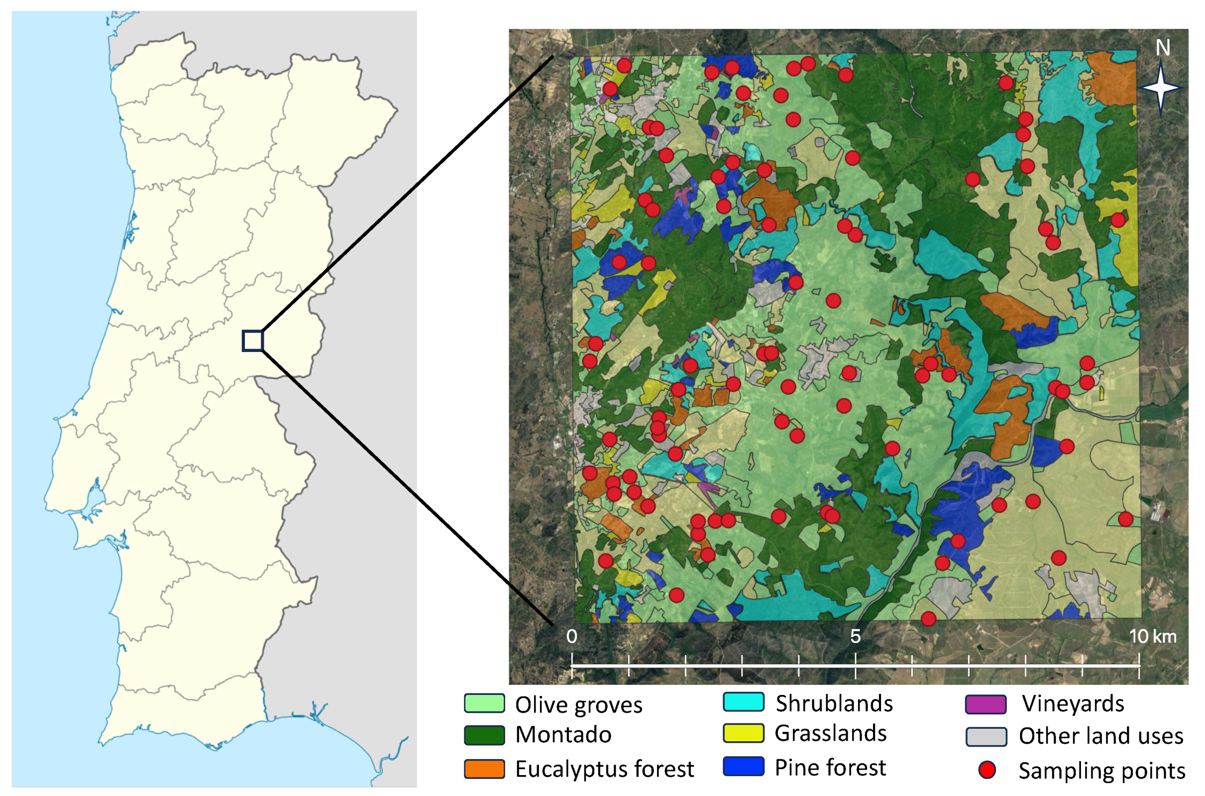
2.1. Study Locations and Insect Sampling

To achieve our research goals, we selected a total of 79 sampling locations distributed across various predominant habitats identified in the Beira Interior region of Portugal, encompassing the municipalities of Castelo Branco and Idanha-a-Nova (Figure 1). The area of study was a square of 10 kms by 10 kms. The habitats observed in this region included shrublands, eucalyptus forests, pine forests, “montado” (Iberian oak savannahs), grasslands, vineyards, and olive groves. Given that olive groves are a crop of major importance in the study area and the relevance that Chrysoperla carnea s.l. has in this crop as a biological control agent, 25 out of the total 79 sampling points were specifically situated within olive groves. In total, 25 olive groves were chosen because this is the typical number of sampling points in these types of studies in olive groves [3,26]. For the rest of the habitats, we deployed nine sampling points per habitat. We distributed these points aiming at covering the whole square of 10 by 10 km. We considered that this number is high enough to give enough representation of the results obtained.
The majority of these olive groves were centennial and consisted mainly of the Galega variety. They were not irrigated and had limited ground cover vegetation due to the presence of livestock. These olive groves were actively cultivated at the time of sampling and each sampling point was located in a single field owned by a single farmer. Notably, no pesticides were applied, and no land-ploughing methods were employed by olive growers during the study. The remaining sampling points were evenly distributed among the other habitat categories, with nine points allocated to each habitat (Figure 1). The minimum distance between points was 588.1 m, while the maximum distance was 10,331.8 m (Figure 1). This minimum distance was chosen because the normal dispersal range of C. carnea s.l. is 500 m per day, although it can reach mora than 10 km in the first stages of its adulthood [21].
To assess the abundance of Chrysoperla carnea s.l., we deployed McPhail traps at each of the selected points in February 2019 (Figure 1). Each trap was baited with a liquid mixture containing 5% diammonium phosphate and 2% borax dissolved in 250 mL of water, a highly effective attractant for C. carnea s.l. adults [27]. At every sampling point, monthly collections were conducted over one year, commencing in February 2019 and concluding in January 2020, specifically on the: 13 February, 17 March, 15 April, 23 May, 20 June, 25 July, 23 August, 20 September, 17 October, 15 November, 12 December, and 26 January. Following field collection, the samples were transported to the laboratory for counting C. carnea s.l. individuals. Chrysoperla carnea s.l. correspond to a set of sibling species that are very difficult to recognize visually on an individual basis. Even molecular methods result in difficult determination. In the olive groves landscape, several species are the most representative of this complex, namely Chrysoperla carnea s.str., Chrysoperla agilis (Henry, Brooks, Duelli & Johnson, 2003), Chrysoperla lucasina (Lacroix, 1912), and Chrysoperla affinis (Henry, Brooks, Duelli & Johnson, 2003) [28]. It is widely recognized that the identification of the species of this complex is very difficult and involves methods that go beyond the scope of this study. In addition, these species share the same functional role [28]. Therefore, throughout the document, we refer to this complex as C.carnea s.l. as this is the convection in these types of studies [29,30].

2.2. Landscape Analysis

Landscape analysis was performed for the 25 sampling points located within olive groves. A geospatial analysis was conducted on the surrounding buffer area within a 500 m radius using QGIS software [31], a Geographic Information Systems (GIS) platform. Aerial photographs were utilized to delineate polygons representing different habitat patches within the study area, as previously mentioned. To validate the accuracy of landscape elements and complement aerial photographs, visual field validation was performed to confirm the habitat at each selected point. All geospatial data were converted into raster images and analyzed using Fragstats software (University of Massachusetts, Amherst, MA, USA). From this spatial pattern analysis, we derived class-level landscape metrics, quantifying the total area of each habitat within the landscape buffer zones as a percentage. These values were used to calculate Shannon’s diversity index (SHDI) as an indicator of landscape diversity. Landscape simplification was estimated by assessing the proportion of olive habitat surrounding each sampling point.

2.3. Statistical Modelling

We simplified and standardized the data by consolidating individual counts for C. carnea s.l. across all sampling dates, resulting in a singular value per sampling point. This approach facilitated the application of statistical models to comprehend the patterns and relationships observed in the study. Statistically significant differences between pairs of habitats were determined using a nonparametric Wilcoxon rank sum test, with p-values adjusted using Benjamini and Hochberg’s method [32]. To enhance representation in a boxplot, the data used for this test were log-transformed.
To examine the dynamics of Chrysoperla carnea s.l. in various habitats over a year, we employed Generalized Additive Mixed Models (GAMMs). These models incorporated an interaction term between the Julian day of trap sampling and the specific habitat where the traps were situated. We used five knots to capture the population fluctuations within each habitat. To address the issue of pseudoreplication stemming from multiple samples taken at the same location at different times of the year, we introduced the trap location as a random factor. Initially, we applied a Poisson error distribution since the response variable involved counts. However, due to overdispersion, we opted for a negative binomial error distribution with a log link function to better account for this overdispersion. To ensure the stability of our models, we separately analyzed the population dynamics for each habitat, yielding consistent and statistically significant results (p-value < 0.05).
To understand the impact of different habitats on C. carnea s.l. abundance in olive groves, we utilized a combined dataset from the initial analysis, which included a single value for each of the 25 sampled olive groves. We employed a model selection approach based on the Akaike information criteria corrected for small sample size (AICc) to identify the most parsimonious model, that is, the one that better explains variance with the lower number of parameters. Models with the lowest AICc, as well as those with a difference of less than two AICc units from the lowest, were considered for further analysis [33]. Consequently, we created a series of generalized linear models (GLM), each incorporating a different habitat as a predictor, such as olive, shrublands, “montado,” grasslands, eucalyptus forest, pine forests, vineyards, and the Shannon diversity index. We complemented this set of models with a null model to account for non-effects. Similar to the population dynamic models, we initially considered a Poisson error distribution, but, after detecting overdispersion, we chose to model the data using a negative binomial error distribution with a log link function.
All analyses were carried out in R, utilizing various packages, including “mgcv” for GAMMs [34], “lme4” for GLMs [35], “DHARMa” for overdispersion analysis [36], and “ggplot2” for result visualization [37].

3. Results

3.1. Abundance of C. carnea s.l. in Different Habitats

Throughout the entire sampling period, a total of 2052 Chrysoperla carnea s.l. individuals were collected. These insects were found across all the habitats examined in the study, as depicted in Figure 2. The highest mean abundance per habitat was found in olive groves (40.97 ± 27.28 individuals per plot) followed very closely by the mean abundance in montado (39.22 ± 33.38 individuals per plot). Except for montado, olive groves displayed significant differences from most of the other habitats as shown by the Wilconson test (Table 1). In the case of montado, it displayed significant differences with shrublands, grasslands and pine forests. The rest of the habitats only showed significant differences with the formerly mentioned habitats, but no differences were found among them (Table 1). Eucalyptus forest displayed a mean abundance of C. carnea s.l. of 15.11 ± 11.01 individuals per plot followed by vineyards (12.00 ± 9.21 individuals per plot), pine forest (9.33 ± 9.15 individuals per plot) and shrubs (8.11 ± 5.93 individuals per plot). The lowest abundance was found in grasslands (7.67 ± 9.29 individuals per plot). These variations are visually represented in Figure 2 and correspond with the results from the Wilcoxon test, as detailed in Table 1.

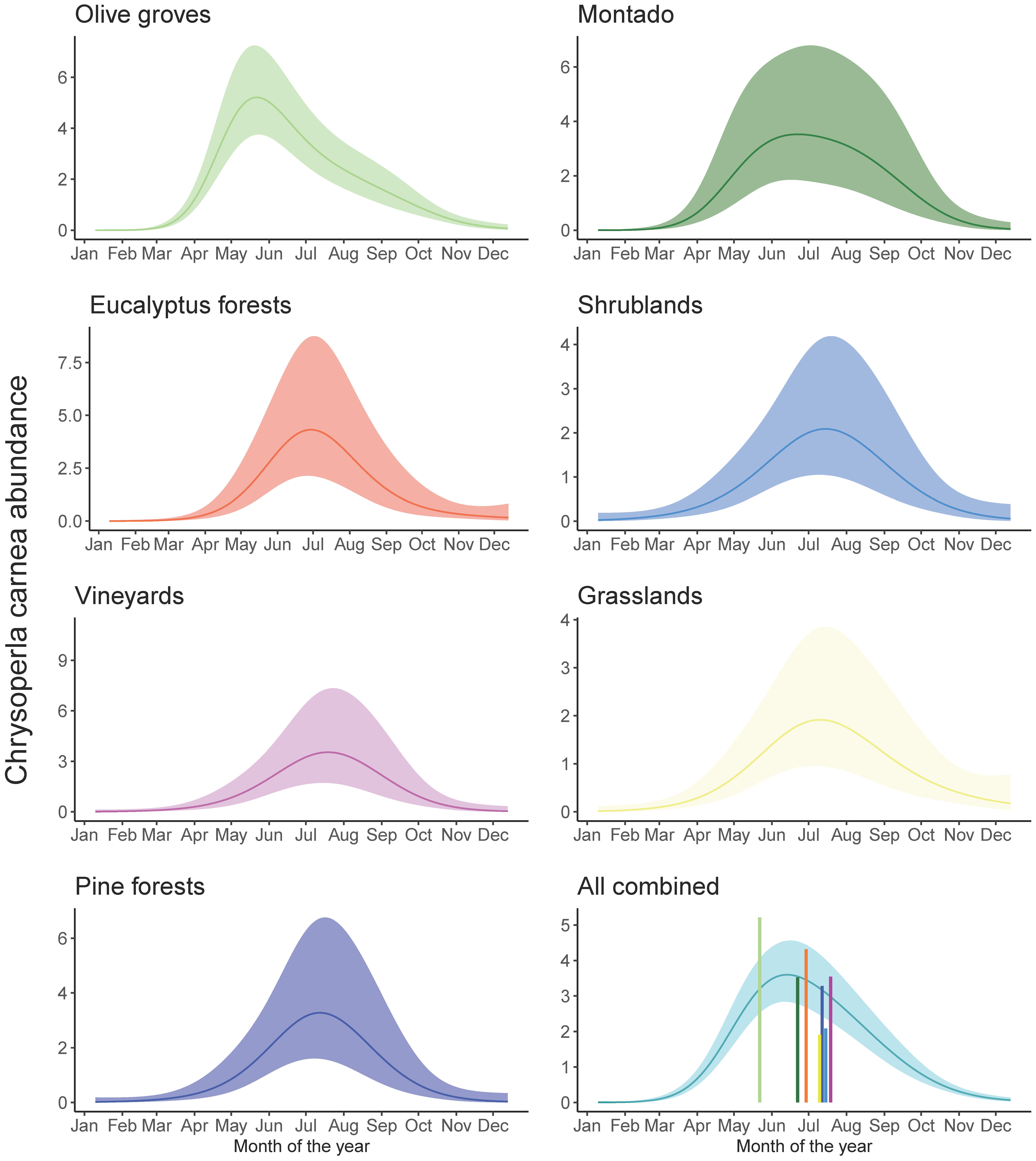
3.2. Temporal Dynamics of C. carnea s.l. in Different Habitats

During the study, we observed significant natural enemy dynamics in all seven habitats investigated (Figure 3). In olive groves, the C. carnea s.l. population peaked sooner than in the rest of the habitats, around mid-May. At this moment, the abundance reached 5.21 individuals/plot, the highest of all analysed habitats (Figure 3). The second habitat in which C. carnea s.l. population peaked was in montado, around mid-June (Figure 3). The peak abundance in montado habitat was 3.52 individuals per plot. These two habitats were in which abundance was higher when the year was analysed as a hold (Figure 2) but have a notable difference in their peaks denoting that montado habitats held a steady abundance of C. carnea s.l. for a longer time than in olive groves, as can be seen in Figure 3. The habitat in which C. carnea s.l. peaked after was the eucalyptus forest, around the beginning of July (Figure 3). Peak abundance in this habitat was 4.32 individuals per plot. Critically, this is the habitat that held the third higher abundance when compared to others, but the shape of the curve is narrower than for montado. For the rest of habitats, C. carnea s.l. populations peaked later, around August; however, it can be noted in Figure 3 that the abundance of this natural enemy reached its maximum a little bit sooner in grasslands. In this habitat, the peak abundance was the lowest of all with 1.91 individuals per plot. In vineyards and pine forests, the peak abundance was very similar to this in montado with 3.54 and 3.28 individuals per plot, respectively (Figure 3). Finally, the peak abundance in shrublands was 2.09 individuals per plot (Figure 3). All combined, the abundance of C. carnea s.l. peaks in mid-June for the entire landscape, reaching a maximum of 3.56 individuals per plot. It is important to note the overall temporal dynamics and how the curve is wider than in the other habitats.

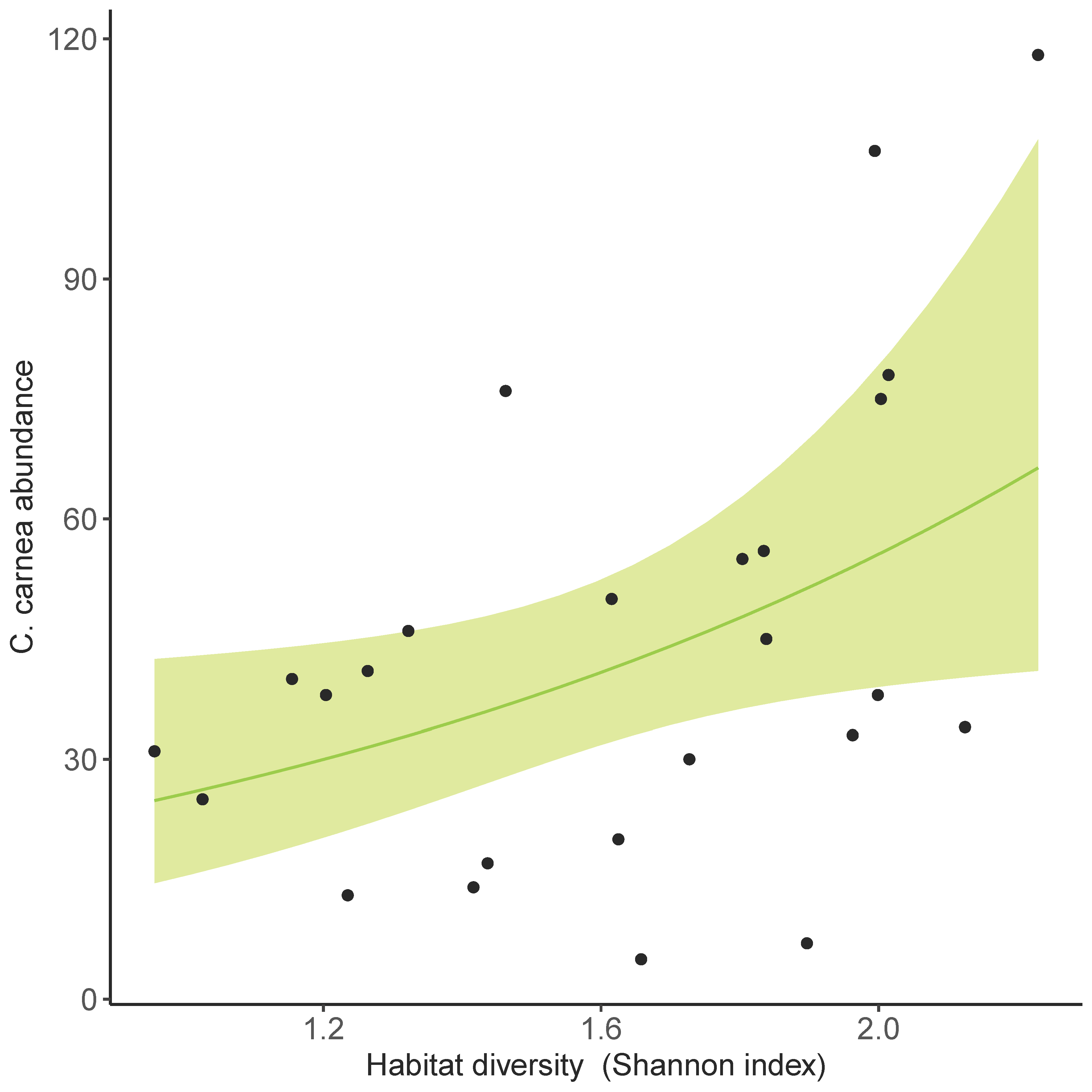
3.3. Land Use Effect on C. carnea s.l. Abundance in Olive Groves

The most parsimonious model explaining the abundance of C. carnea s.l. in olive groves was the one containing the predictor habitat diversity in the landscape (AICc = 233.35; Table 2). There was a notable effect of habitat diversity on Chrysoperla carnea s.l. abundance increasing more than twofold from plots with the lowest habitat diversity to plots with higher habitat diversity (Figure 4). In the model, the habitat diversity showed a significant effect (p-value = 0.022).

4. Discussion

The adoption of landscape-scale habitat diversification strategies to enhance biocontrol services is increasingly viewed as an eco-friendly alternative to the use of chemical products for agricultural management [3,38]. Nevertheless, it is imperative to thoroughly understand the temporal and spatial dynamics of the key contributors to this service. The case of Chrysoperla carnea s.l. is of particular significance. This is because it involves a generalist predator with the capacity to manage a wide array of pests within a crop that has co-evolved with the Mediterranean agricultural landscape for centuries. This presents a significant challenge when formulating landscape-scale habitat diversification strategies [39]. The habitat preferences of this predator may lead it to select habitats other than the target crop, thereby reducing its ability to effectively control olive pests [14].
The findings of this study indicate that C. carnea s.l. is present in all the habitats examined. However, data analysis suggests that it moves through various habitats throughout the year. The peak abundance is initially observed in olive groves, precisely when its preferred prey, Prays oleae [22], is present in the crop. It is worth noting that previous research in the same area demonstrated a significant attraction of C. carnea s.l. to plots with high P. oleae abundance [22]. This study confirms these findings and highlights C. carnea s.l. as an effective biocontrol agent against P. oleae, as its population peaks when the pest is most abundant. Following this, the population starts to decline but peaks sequentially in other habitats, indicating movement patterns. Therefore, from olive groves, C. carnea s.l. moves to montados, then to eucalyptus forests, where its population peaks around the beginning of July. It subsequently spreads to different habitats such as grasslands, shrublands, and pine forests, with a noticeable decrease in peak abundance. The final peak of abundance is observed in vineyards, where C. carnea s.l. may be preying on pests such as Lobesia botrana (Denis & Schiffermüller, 1775) (Lepidoptera: Totricidae) [40,41].
Movements of Chrysoperla carnea s.l. in the landscape are complex. When adults emerge, there is preovipository migration process of around two days in which they disperse in a long-range, downwind, reaching distances that depending on the authors can reach from 10 to an impressive 40 km [21,42]. Therefore, it is difficult to estimate the distance that lacewing adults can fly during this preoviposition period. In contrast, during the oviposition period, Chrysoperla carnea s.l. adults disperse at sunset, by flying approximately 500 m downwind, with the distance also influenced by wind speed but more related to seeking food sources [21,42]. Consequently, the concentration of lacewings in a certain habitat must be ruled by the number of potential food sources that C. carnea can find in that particular habitat [21,42]. Our results show that this is especially clear for olive groves in which there is a high concentration of C. carnea s.l. adults at the beginning of the season, matching with the moment in which the eggs of the carpophagous generation of Prays oleae are laid [43]. The important thing here is to know how we can increase this population in the olive grove during that moment in which that pest is present to achieve optimal control over it. From our results, increasing habitat diversification at the landscape scale seems to be the optimal action to achieve this objective.
Habitat diversity has been seen as a good strategy to increase C. carnea s.l. populations in olive groves [22,44,45]. The reason relies on the fact that diversified landscapes provide more resources for the development of natural enemies [10,11,46], especially pollen [47]. Diverse agricultural landscapes that incorporate a mix of wooded areas and meadows, ensure that there is a varied timing of flowering resources to support insect species that offer C. carnea s.l. the resources it needs across the season [48,49]. Because of this, the abundance of this insect peaks in several habitats at different times, therefore ensuring a substantial amount of resources. This fact aligns with the natural enemy hypothesis that poses that resources at the landscape scale are crucial for optimal natural enemy performance [8,9].
Management implications of these findings prove challenging, particularly due to the complexities associated with conducting landscape planning over an extended period. This highlights the need for policymakers and stakeholders to refine their strategies to boost Chrysoperla carnea s.l. abundance in olive groves. On an individual level, farmers can contribute by integrating indigenous vegetation within and around their farms to enhance C. carnea s.l. abundance. Also, when planning new olive plantations, new policies could make farmers allocate a specific portion of the new crop to other crops or semi-natural habitats, thus increasing habitat diversity. Yet, achieving a more widespread increase in habitat diversity at the landscape scale requires collaboration among neighbouring farmer groups. While this may involve certain expenses, structured compensation programs can be employed to encourage farmers’ cooperation in enhancing landscape complexity [50]. This would help steer clear of monoculture, consequently promoting habitat diversification. This collaborative, landscape-informed approach to pest management represents a significant advancement crucial for realizing tangible benefits in sustainable olive production, farmland conservation, and human well-being. Looking ahead, future efforts should be directed towards elevating habitat diversity at the landscape scale, emphasizing the importance of this strategy for stakeholders aiming to augment Chrysoperla carnea abundance in olive groves and mitigate significant pest issues in this crop and, consequently, pesticide applications [3].

5. Conclusions

The study concludes that understanding the spatial and temporal dynamics of key contributors to biocontrol services, specifically Chrysoperla carnea s.l., is crucial. Despite being a significant generalist predator in managing pests in the Mediterranean agricultural landscape, its habitat preferences present challenges in devising effective landscape-scale habitat diversification strategies. The research uncovers the intricate movements of C. carnea s.l. across various habitats throughout the year, with peaks in olive groves corresponding to the presence of its preferred prey. The results underscore the importance of increasing habitat diversification at the landscape scale for optimal natural enemy performance, aligning with the natural enemy hypothesis [8,9]. Implementing such strategies requires collaboration among farmers, policymakers, and stakeholders, emphasizing the need for structured compensation programs and collective efforts to enhance landscape complexity. Overall, these findings advocate for a holistic approach to pest management, recognizing the pivotal role of habitat diversity in sustaining Chrysoperla carnea s.l. populations and promoting sustainable olive production.

Author Contributions

D.P., S.M. and J.P.S. conceived the project and designed the methods; D.P. and S.M. collected the data; D.P. and J.P.S. analyzed the data; D.P. wrote the study. All authors made critical contributions to the draft and gave final approval for publication. All authors have read and agreed to the published version of the manuscript.

Funding

This research was funded by Programa Operacional Regional do Centro, Grant Number Centro-01-0145-FEDER-000007 (ReNATURE), by the European Union’s Horizon 2020 Research and Innovation Programme, under Grant Agreement No. 773554 (EcoStack), and by Fundação para a Ciência e Tecnologia through the project PTDC/ASP-PLA/30003/2017 (OLIVESIM) This work was also supported by FCT - Fundação para a Ciência e Tecnologia, I.P. by project reference UIDB/04004/2020 and DOI identifier 10.54499/UIDB/04004/2020 (https://doi.org/10.54499/UIDB/04004/2020). The APC was funded by European Union’s Horizon 2020 Research and Innovation Programme, underGrant Agreement No. 773554 (EcoStack).

Institutional Review Board Statement

The study did not require ethical approval.

Data Availability Statement

Data will be available upon request.

Acknowledgments

The authors would also like to express their appreciation to the Association of Olive Oil Producers of Beira Interior (APABI, Portugal) for diligently identifying and locating the necessary landowners. They are also thankful to the olive growers who graciously permitted the traps to be placed on their properties during the trial period. Special thanks go to Mikola Rasko, Rúben Mina, and Sandra Simões for their valuable contributions to the sampling process.

Conflicts of Interest

The authors declare no conflicts of interest.

References

  1. Foley, J.A.; DeFries, R.; Asner, G.P.; Barford, C.; Bonan, G.; Carpenter, S.R.; Chapin, F.S.; Coe, M.T.; Daily, G.C.; Gibbs, H.K.; et al. Global Consequences of Land Use. Science 2005, 309, 570–574. [Google Scholar] [CrossRef]
  2. Dirzo, R.; Young, H.S.; Galetti, M.; Ceballos, G.; Isaac, N.J.B.; Collen, B. Defaunation in the Anthropocene. Science 2014, 345, 401–406. [Google Scholar] [CrossRef] [PubMed]
  3. Paredes, D.; Rosenheim, J.A.; Chaplin-Kramer, R.; Winter, S.; Karp, D.S. Landscape Simplification Increases Vineyard Pest Outbreaks and Insecticide Use. Ecol. Lett. 2021, 24, 73–83. [Google Scholar] [CrossRef]
  4. Gould, F.; Brown, Z.S.; Kuzma, J. Wicked Evolution: Can We Address the Sociobiological Dilemma of Pesticide Resistance? Science 2018, 360, 728–732. [Google Scholar] [CrossRef]
  5. European Commission. A Farm to Fork Strategy for a Fair, Healthy and Enviromental-Friendly System; European Commission: Brussels, Belgium, 2020; Volume 21, pp. 1–9. [Google Scholar]
  6. Thies, C.; Tscharntke, T. Landscape Structure and Biological Control in Agroecosystems. Science 1999, 285, 893–895. [Google Scholar] [CrossRef]
  7. Bianchi, F.J.J.A.; Booij, C.J.H.; Tscharntke, T. Sustainable Pest Regulation in Agricultural Landscapes: A Review on Landscape Composition, Biodiversity and Natural Pest Control. Proc. Royal Soc. B-Biol. Sci. 2006, 273, 1715–1727. [Google Scholar] [CrossRef]
  8. Russell, E.P. Enemies Hypothesis: A Review of the Effect of Vegetational Diversity on Predatory Insects and Parasitoids; The University of Kansas: Lawrence, KS, USA, 1989; Volume 18. [Google Scholar]
  9. Chaplin-Kramer, R.; O’Rourke, M.E.; Blitzer, E.J.; Kremen, C. A Meta-Analysis of Crop Pest and Natural Enemy Response to Landscape Complexity. Ecol. Lett. 2011, 14, 922–932. [Google Scholar] [CrossRef] [PubMed]
  10. Landis, D.A.; Wratten, S.D.; Gurr, G.M. Habitat Management to Conserve Natural Enemies of Arthropod Pests in Agriculture. Annu. Rev. Entomol. 2000, 45, 175–201. [Google Scholar] [CrossRef] [PubMed]
  11. Gurr, G.M.; Wratten, S.D.; Landis, D.A.; You, M. Habitat Management to Suppress Pest Populations: Progress and Prospects. Annu. Rev. Entomol. 2017, 62, 91–109. [Google Scholar] [CrossRef]
  12. Ferrante, M.; González, E.; Lövei, G.L. Predators Do Not Spill over from Forest Fragments to Maize Fields in a Landscape Mosaic in Central Argentina. Ecol. Evol. 2017, 7, 7699–7707. [Google Scholar] [CrossRef]
  13. Blitzer, E.J.; Dormann, C.F.; Holzschuh, A.; Klein, A.M.; Rand, T.A.; Tscharntke, T. Spillover of Functionally Important Organisms between Managed and Natural Habitats. Agric. Ecosyst. Environ. 2012, 146, 34–43. [Google Scholar] [CrossRef]
  14. Thomine, E.; Rusch, A.; Supplisson, C.; Monticelli, L.S.; Amiens-Desneux, E.; Lavoir, A.-V.; Desneux, N. Highly Diversified Crop Systems Can Promote the Dispersal and Foraging Activity of the Generalist Predator Harmonia Axyridis. Entomol. Gen. 2020, 40, 133–145. [Google Scholar] [CrossRef]
  15. Symondson, W.O.C.; Sunderland, K.D.; Greenstone, M.H. Can Generalist Predators Be Effective Biocontrol Agents? Annu Rev. Entomol. 2002, 47, 561–594. [Google Scholar] [CrossRef] [PubMed]
  16. Snyder, W.E.; Ives, A.R. Generalist Predators Disrupt Biological Control by a Specialist Parasitoid. Ecology 2001, 82, 705. [Google Scholar] [CrossRef]
  17. Snyder, W.E. Give Predators a Complement: Conserving Natural Enemy Biodiversity to Improve Biocontrol. Biol. Control. 2019, 135, 73–82. [Google Scholar] [CrossRef]
  18. Welch, K.D.; Harwood, J.D. Temporal Dynamics of Natural Enemy–Pest Interactions in a Changing Environment. Biol. Control. 2014, 75, 18–27. [Google Scholar] [CrossRef]
  19. Rosenheim, J.A.; Limburg, D.D.; Colfer, R.G. Impact of generalist predators on a biological control agent, Chrysoperla carnea: Direct observations. Ecol. Appl. 1999, 9, 409–417. [Google Scholar] [CrossRef]
  20. Atlihan, R.; Kaydan, B.; Özgökçe, M.S. Feeding Activity and Life History Characteristics of the Generalist Predator, Chrysoperla Carnea (Neuroptera: Chrysopidae) at Different Prey Densities. J. Pest. Sci. 2004, 77, 17–21. [Google Scholar] [CrossRef]
  21. Duelli, P. Dispersal and Opposition Strategies in Chrysoperla Carnea. In Progress in World´s Neuroptera; Johann Gepp: Graz, Austria, 1984. [Google Scholar]
  22. Alves, J.F.; Mendes, S.; da Silva, A.A.; Sousa, J.P.; Paredes, D. Land-Use Effect on Olive Groves Pest Prays Oleae and on Its Potential Biocontrol Agent Chrysoperla Carnea. Insects 2021, 12, 46. [Google Scholar] [CrossRef]
  23. Paredes, D.; Cayuela, L.; Gurr, G.M.; Campos, M. Effect of Non-Crop Vegetation Types on Conservation Biological Control of Pests in Olive Groves. PeerJ 2013, 2013, e116. [Google Scholar] [CrossRef]
  24. Paredes, D.; Cayuela, L.; Gurr, G.M.; Campos, M. Single Best Species or Natural Enemy Assemblages? A Correlational Approach to Investigating Ecosystem Function. BioControl 2015, 60, 37–45. [Google Scholar] [CrossRef]
  25. Kubiak, K.L.; Pereira, J.A.; Tessaro, D.; Santos, S.A.P.; Benhadi-Marín, J. The Assemblage of Beetles in the Olive Grove and Surrounding Mediterranean Shrublands in Portugal. Agriculture 2022, 12, 771. [Google Scholar] [CrossRef]
  26. Rosenheim, J.A.; Cluff, E.; Lippey, M.K.; Cass, B.N.; Paredes, D.; Parsa, S.; Karp, D.S.; Chaplin-Kramer, R. Increasing Crop Field Size Does Not Consistently Exacerbate Insect Pest Problems. Proc. Natl. Acad. Sci. USA 2022, 119, e2208813119. [Google Scholar] [CrossRef] [PubMed]
  27. Porcel, M.; Ruano, F.; Sanllorente, O.; Caballero, J.A.; Campos, M. Comunicación Corta. Efecto del Trampeo Masivo Tipo OLIPE Sobre Los Artrópodos No Objetivo del Olivar. SJAR 2009, 7, 660–664. [Google Scholar] [CrossRef]
  28. Bozsik, A.; González-Ruíz, R.; Hurtado-Lara, B. Distribution of the Chrysoperla Carnea Complex in Southern Spain (Neuroptera: Chrysopidae); University of Oradea Publishing House: Oradea, Romania, 2009. [Google Scholar]
  29. Villa, M.; Somavilla, I.; Santos, S.A.P.; López-Sáez, J.A.; Pereira, J.A. Pollen Feeding Habits of Chrysoperla Carnea s.l. Adults in the Olive Grove Agroecosystem. Agric. Ecosyst. Environ. 2019, 283, 106573. [Google Scholar] [CrossRef]
  30. Villa, M.; Santos, S.A.P.; Benhadi-Marín, J.; Mexia, A.; Bento, A.; Pereira, J.A. Life-History Parameters of Chrysoperla Carnea s.l. Fed on Spontaneous Plant Species and Insect Honeydews: Importance for Conservation Biological Control. BioControl 2016, 61, 533–543. [Google Scholar] [CrossRef]
  31. QGIS.org. QGIS Geographic Information System. Open Source Geospatial Foundation Project. 2019. Available online: http://qgis.osgeo.org (accessed on 16 January 2024).
  32. Benjamini, J.; Hochberg, Y. Controlling the false discovery rate: A practical and powerful approach to multiple testing. J. R. Stat. Soc. Series B Stat. Methodol. 1995, 57, 89–300. [Google Scholar] [CrossRef]
  33. Burnham, K.P.; Anderson, D.R. Model Selection and Multimodel Inference; Springer: New York, NY, USA, 2004. [Google Scholar] [CrossRef]
  34. Wood, S.N. Fast Stable Restricted Maximum Likelihood and Marginal Likelihood Estimation of Semiparametric Generalized Linear Models. J. R. Stat. Soc. Series B Stat. Methodol. 2011, 73, 3–36. [Google Scholar] [CrossRef]
  35. Bates, D.; Mächler, M.; Bolker, B.M.; Walker, S.C. Fitting Linear Mixed-Effects Models Using Lme4. J. Stat. Softw. 2015, 67, 48. [Google Scholar] [CrossRef]
  36. Harting F DHARMa: Residual Diagnostics for Hierarchical (Multi-Level/Mixed) Regression Models. Available online: https://cran.r-project.org/web/packages/DHARMa/vignettes/DHARMa.html (accessed on 6 November 2023).
  37. Wickham, H. Ggplot2: Elegant Graphics for Data Analysis; Springer: New York, NY, USA, 2016. [Google Scholar]
  38. Thomine, E.; Mumford, J.; Rusch, A.; Desneux, N. Using Crop Diversity to Lower Pesticide Use: Socio-Ecological Approaches. Sci. Total Environ. 2022, 804, 150156. [Google Scholar] [CrossRef]
  39. Gurr, G.M.; Lu, Z.; Zheng, X.; Xu, H.; Zhu, P.; Chen, G.; Yao, X.; Cheng, J.; Zhu, Z.; Catindig, J.L.; et al. Multi-Country Evidence That Crop Diversification Promotes Ecological Intensification of Agriculture. Nat. Plants 2016, 2, 1–4. [Google Scholar] [CrossRef]
  40. Thiéry, D.; Moreau, J. Relative Performance of European Grapevine Moth (Lobesia botrana) on Grapes and Other Hosts. Oecologia 2005, 143, 548–557. [Google Scholar] [CrossRef]
  41. Serée, L.; Rouzes, R.; Thiéry, D.; Rusch, A. Temporal Variation of the Effects of Landscape Composition on Lacewings (Chrysopidae: Neuroptera) in Vineyards. Agric. For. Entomol. 2020, 22, 274–283. [Google Scholar] [CrossRef]
  42. Duelli, P. Lacewings in Field Crops. In Lacewings in the Crop Environment; Cambridge University Press: Cambridge, UK, 2001; pp. 158–171. [Google Scholar]
  43. Gómez-Guzmán, J.A.; Herrera, J.M.; Rivera, V.; Barreiro, S.; Muñoz-Rojas, J.; García-Ruiz, R.; González-Ruiz, R. A Comparison of IPM and Organic Farming Systems Based on the Efficiency of Oophagous Predation on the Olive Moth (Prays Oleae Bernard) in Olive Groves of Southern Iberia. Horticulturae 2022, 8, 977. [Google Scholar] [CrossRef]
  44. Alcalá Herrera, R.; Ruano, F. Impact of Woody Semi-Natural Habitats on the Abundance and Diversity of Green Lacewings in Olive Orchards. Biol. Control 2022, 174, 105003. [Google Scholar] [CrossRef]
  45. Paredes, D.; Karp, D.S.; Chaplin-Kramer, R.; Benítez, E.; Campos, M. Natural Habitat Increases Natural Pest Control in Olive Groves: Economic Implications. J. Pest. Sci. 2019, 92, 1111–1121. [Google Scholar] [CrossRef]
  46. Dainese, M.; Martin, E.A.; Aizen, M.A.; Albrecht, M.; Bartomeus, I.; Bommarco, R.; Carvalheiro, L.G.; Chaplin-Kramer, R.; Gagic, V.; Garibaldi, L.A.; et al. A Global Synthesis Reveals Biodiversity-Mediated Benefits for Crop Production. Sci. Adv. 2019, 5, eaax0121. [Google Scholar] [CrossRef] [PubMed]
  47. Bertrand, C.; Eckerter, P.W.; Ammann, L.; Entling, M.H.; Gobet, E.; Herzog, F.; Mestre, L.; Tinner, W.; Albrecht, M. Seasonal Shifts and Complementary Use of Pollen Sources by Two Bees, a Lacewing and a Ladybeetle Species in European Agricultural Landscapes. J. App. Ecol. 2019, 56, 2431–2442. [Google Scholar] [CrossRef]
  48. Fountain, M.T. Impacts of Wildflower Interventions on Beneficial Insects in Fruit Crops: A Review. Insects 2022, 13, 304. [Google Scholar] [CrossRef] [PubMed]
  49. Karamaouna, F.; Kati, V.; Volakakis, N.; Varikou, K.; Garantonakis, N.; Economou, L.; Birouraki, A.; Markellou, E.; Liberopoulou, S.; Edwards, M. Ground Cover Management with Mixtures of Flowering Plants to Enhance Insect Pollinators and Natural Enemies of Pests in Olive Groves. Agric. Ecosyst. Environ. 2019, 274, 76–89. [Google Scholar] [CrossRef]
  50. Batáry, P.; Dicks, L.V.; Kleijn, D.; Sutherland, W.J. The Role of Agri-Environment Schemes in Conservation and Environmental Management. Conserv. Biol. 2015, 29, 1006–1016. [Google Scholar] [CrossRef] [PubMed]
Figure 1. The left panel shows the study area’s position in Portugal, while the right panel illustrates the arrangement of sampling locations throughout the various land types within the study area.
Agriculture 14 00298 g001
Figure 2. Boxplot illustrating the logarithmic values of Chrysoperla carnea s.l. (common green lacewing) abundance across various habitats investigated in this study. Within each box, the top and bottom lines represent the first quartile (Q1) and third quartile (Q3), respectively, while the middle line indicates the median (Q2). The whiskers extending from the boxes denote values up to 1.5 times the interquartile range, calculated as the difference between Q3 and Q2 for the upper and lower quartiles. Additionally, individual points on the plot correspond to the logarithmic abundance recorded at each sampling location.
Agriculture 14 00298 g002
Figure 3. Temporal dynamics of Chrysoperla carnea s.l. within the various habitats that make up the study, as well as an overview of all these dynamics combined. The light green line represents olive groves, dark green represents “montados”, the orange line represents eucalyptus forests, the light blue line represents shrublands, the violent line represents vineyards, the light-yellow line represents grasslands, the dark blue line represents pine forests, and the cyan line represents the dynamics of C. carnea s.l. in all habitats combined without any distinction. Also, in the bottom right plot, bars correspond in the x-axis with the moment in which maximum abundance was reached. That abundance corresponds with the height of the bar. Bar colors are the same as for the habitats represented in this figure. Shadowed areas represent the confidence intervals at 95%.
Agriculture 14 00298 g003
Figure 4. Estimated effects of the gradient of habitat diversity, calculated with the Shannon diversity index, on the abundance of Chrysoperla carnea s.l. Shadowed areas represent the confidence intervals at 95% (N = 25).
Agriculture 14 00298 g004
Table 1. Statistically significant differences between pairs of habitats. These differences were determined through a nonparametric Wilcoxon rank-sum test, and the associated p-values were adjusted using Benjamini and Hochberg’s method.
Eucalyptus ForestsShrublandsMontadoOlive grovesGrasslandsPine Forests
Shrublands0.465
Montado0.1780.031
Olive groves0.011<0.0010.816
Grasslands0.2970.5570.014<0.001
Pine forests0.5571.0000.031<0.0010.557
Vineyards0.6250.5570.0710.0040.4650.625
Note: Statistical significant values in bold.
Table 2. Akaike information criteria corrected for small sample size for the generalized linear model account for the effect of the proportion of surrounding habitats on the population of Chrysoperla carnea s.l. in olive groves. The lowest value is in bold.
HabitatAICc
Null236.00
Montado238.56
Eucalyptus forests237.29
Grasslands236.54
Pine forests237.44
Shrublands237.41
Vineyards238.29
Olive groves238.59
Habitat diversity (Shannon index)233.35
Disclaimer/Publisher’s Note: The statements, opinions and data contained in all publications are solely those of the individual author(s) and contributor(s) and not of MDPI and/or the editor(s). MDPI and/or the editor(s) disclaim responsibility for any injury to people or property resulting from any ideas, methods, instructions or products referred to in the content.

