Configuration Optimization of Temperature–Humidity Sensors Based on Weighted Hilbert–Schmidt Independence Criterion in Chinese Solar Greenhouses

Abstract

For cost-sensitive Chinese solar greenhouses (CSGs) with an uneven spatial distribution in temperature and humidity, there is a lack of effective strategies for sensor configuration that can reduce sensor usage while monitoring the microclimate precisely. A configuration strategy for integrated temperature–humidity sensors (THSs) based on the improved weighted Hilbert–Schmidt independence criterion (HSIC) is proposed in this paper. The data independence of the THSs in different sites was analyzed based on the improved HSIC, and the selection priority of the THSs was ranked based on the weighted independence of temperature and humidity. Then, according to different cost constraints and monitoring requirements, suitable THSs could be selected sequentially and constitute the monitoring solution. Compared with the original monitoring solution containing twenty-two THSs, the optimized solution used only four THSs (S6, S9 and H6, H5) under strict cost constraints, with a maximum RMSE of the temperature and relative humidity of 0.6 °C and 2.30%, as well as a maximum information gain rate (IGR) of 9.47% and 10.0%. If higher monitoring precision is required, we can increase the THS usage with a greater budget. The optimized solution with six THSs (S6, S9, S8 and H6, H5, H2) could further reduce the maximum RMSE of the temperature and relative humidity to 0.33 °C and 1.10% and the IGR to 6.9% and 8.7%. This indicated that the proposed strategy could use much fewer THSs to achieve accurate and comprehensive monitoring, which would provide efficient and low-cost solutions for CSG microclimate monitoring.

1. Introduction

As of 2022, Chinese solar greenhouses (CSGs) account for 29% of Chinese facilities’ agriculture cultivation areas. During cold winters, these are an important way to provide fresh vegetables and fruits in the Huang-Huai-Hai Plain and northeast and northwest regions of China [1]. Proper temperature and relative humidity are two key microclimate factors for guaranteeing crop yield and quality in CSGs [2]. The accurate and comprehensive monitoring of temperature and humidity is a prerequisite for the precise regulation of the CSG microclimate and proper field management.

Nowadays, there are three main ways to monitor the aforementioned factors: single point, uniformly multi-point and physically topological point. Benefitting from the advantages of low cost and easy operation, the monitoring method with a single offline thermo-hygrometer placed in the middle point of the greenhouse is widely used in practical production. However, it can only use single-point data to represent the mean temperature and relative humidity of the greenhouse and cannot reflect the spatial distribution of temperature and humidity. Recent research revealed that there are large spatial variations in temperature and humidity inside the greenhouse, which significantly influences crop physiological activity [3]. In the absence of rational microclimate regulation, the temperature and humidity heterogeneity could cause obvious differences in the crop yield and quality in different regions in the greenhouses [4], and low local temperatures could cause irreversible crop damage or even death [5,6]. Therefore, in order to purposely regulate the greenhouse microclimate, not only the mean value but also the spatial distribution of temperature and humidity should be monitored. In order to fully reflect the spatial information, uniformly multi-point [7,8] and physically topological-point methods [9,10] were adopted in some studies. What these two methods have in common is that a large number of sensors, up to 900 sensors, were deployed. Thus, these two methods are more suitable for cost-insensitive study scenarios but are not suitable for cost-sensitive practical greenhouses. It is essential to optimize sensor configuration for the accurate and comprehensive monitoring of temperature and humidity with as few sensors as possible, which would meet the dual requirements of precise monitoring and low investment.

Many meaningful works for optimizing sensor configuration have been carried out in both facility agriculture scenarios and similar industrial scenarios. According to the analysis of temperature spatial distribution based on a computational fluid dynamics (CFD) simulation, the temperature sensors were suggested to be installed at the locations with the lowest gradient of temperature and airflow velocity [11,12]. With the objective of maximizing the monitoring coverage area, temperature sensors and air pollutant sensors were optimized for deployment, respectively, which helped the full exploitation of the monitoring capabilities of the sensor unit and reduced sensor quantity [13,14,15,16]. With the rapid development of machine learning and artificial intelligence, the configurations of temperature sensors and CO₂ sensors were, respectively, optimized in large stadiums and other buildings with the use of different algorithms [17,18,19]. Furthermore, information entropy theory is also a feasible and promising method to optimize sensor configuration and save sensor consumption [20].

Because integrated temperature–humidity sensors (THSs) are widely used in CSGs under strict cost constraints, the above-mentioned methods for single-point sensors are not applicable to THS configuration optimization. Therefore, to achieve the accurate and comprehensive monitoring of a CSG microclimate with limited THS quantity, we propose a THS configuration strategy based on the improved weighted Hilbert–Schmidt independence criterion (HSIC). The independence of different sensors from different areas was evaluated based on the HSIC. Then, the selection priority of the THSs was determined according to the independence ranking. Furthermore, a dual threshold value was proposed and used to determine the number of sensors deployed, which was calculated according to the RMSE and IGR. Finally, the effectiveness of the proposed configuration strategy was verified with test data.

2. Materials and Methods

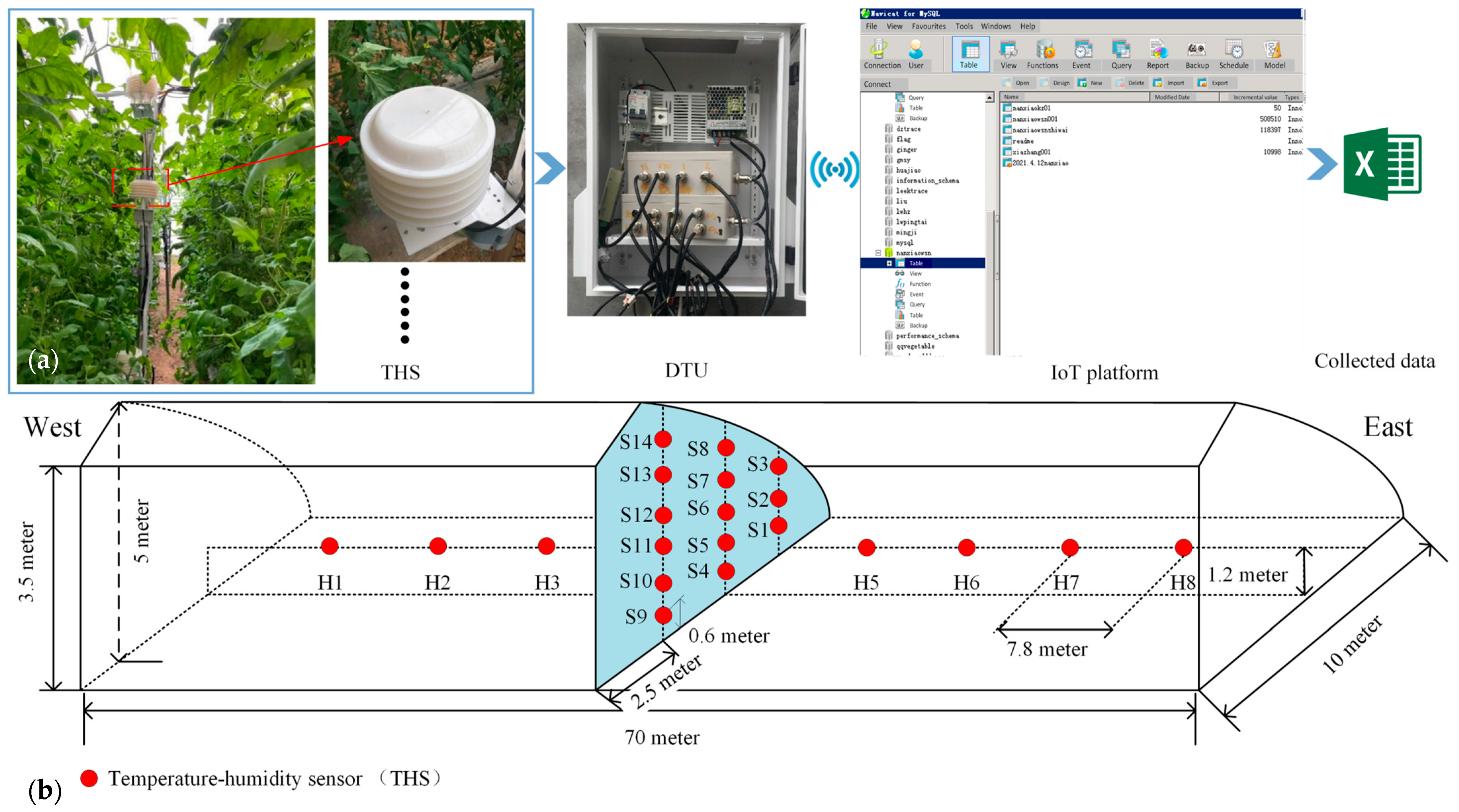
2.1. Introduction of the Test CSG

The implementation and validation of the proposed configuration strategy need temperature and humidity data, so a test CSG for data collection is used in this work. It is located at South Campus of Shandong Agricultural University, Tai’an, Shandong Province, China (117.16° E, 36.16° N), where the outdoor temperature is about −15~10 °C and the indoor temperature is about 5~30 °C in winter. The CSG is planted with tomatoes, with an east–west length of 70 m, a north–south span of 10 m, a ridge height of 5 m, and a north wall height of 3.5 m. The walls are made of brick and concrete, the arches are made of steel, and the covering layer is polyvinyl chloride film, which is covered with an insulation blanket at night for heat preservation. The CSG has two vents at the top and bottom, respectively, and the lower vent is generally closed in winter, and only part of the upper vent is opened for short-term ventilation in the morning when there is sufficient sunlight. The experiment was carried out during a typical cold period in winter (9 December 2020 to 6 January 2021), and 28-day temperature and humidity data were collected for THS configuration optimization.

2.2. Temperature and Humidity Data Collection in the CSG

To collect temperature and humidity data, an IoT system was developed and deployed in the experimental CSG. The system included 22 THSs (DB171-10, Dalian North Measurement and Control, temperature accuracy: ±0.3 °C, range from −20 °C to 80 °C, relative humidity accuracy: 2%, range from 0~100%), 3 data transfer units (DTUs) (H7710D, Shenzhen Hongdian, Shenzhen, China), and a data monitoring platform, as shown in Figure 1a. At the same time, outdoor meteorological-environment-monitoring equipment was installed outside the CSG.

Through the preliminary analysis of the measured data, we found that the temperature and humidity gradient in the north–south vertical direction of the CSG is larger than that in the east–west horizontal direction. Therefore, inspired by the uniform grid configuration, the iso-gradient mode is used in the initial THS configuration. A north–south vertical plane and an east–west horizontal plane were then selected for sensor deployment. The irregular vertical plane is divided by 3 lines along the north–south direction and 6 lines along the vertical direction. Then there are 14 intersection points, each of which has a THS. With respect to the horizontal plane, considering the structural symmetry of the solar greenhouse and the small temperature and humidity gradient, 8 THSs were equally spaced along the east–west direction. Considering the average height of the crop canopy during the monitoring period, the mounting height of the THSs in the east–west direction was set at 1.2 m, as shown in Figure 1b. Temperature and humidity data were collected continuously every 5 min for 28 days × 24 h. After data cleaning and pre-processing, 7880 × 22 sets of temperature and humidity data were obtained.

2.3. Optimization Strategy for THS Configuration

The aim of the THS configuration optimization is to achieve high monitoring accuracy and information abundance of temperature and humidity while reducing the THS usage. Firstly, the weighted HSIC algorithm is proposed to evaluate the priority of all the THSs and to rank them. Secondly, the number of THSs required is determined according to the monitoring accuracy and information abundance requirements. Thirdly, the specific THSs are selected based on the ranking and the required number. Finally, the appropriate THS configurations are constructed to meet different cost constraints and monitoring accuracy requirements.

2.3.1. Monitoring Independence of the THSs

The CSG usually has a large interior space, 2400 m³ for our test, surrounded by several boundaries with different thermal characteristics. Meanwhile, all sub-areas of the CSG are interconnected and interact with each other. The temperature and humidity information from different sites has a high spatial correlation. There is information redundancy of different THSs, which provides improvement potential for optimizing THS configuration and reducing the usage. For the complex nonlinear characteristic of CSG microclimate, we proposed an improved weighted HSIC strategy to optimize the THS configuration.

The HSIC is a kernel-based independence measure, with the advantages of fast convergence, robustness, and low sensitivity to outliers, which is simpler than other kernel-based independence measures and does not require regularization [21]. It can better reflect the nonlinear correlation between the variables [8]. The basic principle is to compute the Hilbert–Schmidt mutual covariance operator on the reproducing kernel Hilbert space (RKHS), and the independence judgment criterion is obtained by empirically estimating the norm of this operator. The higher the calculated HSIC value, the lower the independence of the two variables, i.e., the greater the dependence of the two variables [22]. The HSIC can be used as a basic assessment of the independence of THSs at different sites in the CSG.

Suppose that, $X$, $Y$ are two sets of observable variables, $x\in X,y\in Y$, f(x) and g(y) are two functions that take elements from the sets X and Y as inputs, respectively, and map them onto the set of real numbers $ℝ$, where $f(x),g(y)\in ℝ$, and $p(x,y)$ is the probability density functions of x and y, then for any $f(x),g(y)\in ℝ$, the covariance operator is:

$$\begin{array}{cc}C[f,g]& ={\displaystyle \iint p(x,y)f(x)g(y)dxdy-{\displaystyle \iint p(x)p(y)f(x)g(y)dxdy}}\\ & ={\mathrm{E}}_{(x,y)~p(x,y)}[f(x)g(y)]-{\mathrm{E}}_{x~p(x)}[f(x)]{\mathrm{E}}_{y~p(y)}[g(y)]\hfill \end{array}$$

(1)

If $p(x,y)=p(x)p(y)$, $C[f,g]=0$, x and y are independent of each other. And, conversely, if $p(x,y)\ne p(x)p(y)$, then $C[f,g]\ne 0$, x and y are correlated. The loss function reflects the degree of mutual independence between two variables x and y. Define the loss function as:

$$L_H={\displaystyle \sum _{f,g}{(C[f,g])}^2}$$

(2)

$$\begin{array}{cc}{(C[f,g])}^2& ={({\mathrm{E}}_{(x,y)~p(x,y)}[f(x)g(y)])}^2+{({\mathrm{E}}_{x~p(x)}[f(x)])}^2{({\mathrm{E}}_{y~p(y)}[g(y)])}^2\\ & -2({\mathrm{E}}_{(x,y)~p(x,y)}[f(x)g(y)])({\mathrm{E}}_{x~p(x)}[f(x)])({\mathrm{E}}_{y~p(y)}[g(y)])\hfill \end{array}$$

(3)

To ensure the traversal of $f(x),g(y)$, all possible $f(x)$ compose vector spaces F, all possible $g(y)$ compose vector spaces G, F and G belong to the RKHS; define the nonlinear mapping spaces $\phi (x)\in F$, $\psi (y)\in G$, and $x\in X$, $y\in Y$ and the corresponding kernel functions are denoted as follows, respectively [23].

$$\begin{array}{l}{K}_X(x,x^{\prime })=〈\phi (x),\phi (x^{\prime })〉={\displaystyle \sum _i{\alpha }_i{\phi }_i(x){\phi }_i(x\prime )},x,x^{\prime }\in X\\ K_Y(y,y^{\prime })=〈\psi (y),\psi (y^{\prime })〉={\displaystyle \sum _i{\beta }_i{\psi }_i(y){\psi }_i(y\prime )},y,y^{\prime }\in Y\end{array}$$

(4)

where ${\phi }_1,{\phi }_2,\cdots$ are all the eigenfunctions of the kernel function $K_X$ that form a set of orthogonal bases of the space F, and ${\alpha }_1,{\alpha }_2,\cdots$ are all the eigenvalues of the kernel function $K_X$ that are positive. Similarly, ${\psi }_1,{\psi }_2,\cdots$ are all the eigenfunctions of the kernel function $K_Y$ that form a set of orthogonal bases of the space G, and ${\beta }_1,{\beta }_2,\cdots$ are all the eigenvalues of the kernel function $K_Y$ that are positive.

Therefore, $f(x),g(y)$ can be expressed as a linear combination of orthogonal bases, and the loss function in Equation (2) can be expressed as:

$$L_H={\displaystyle \sum _{i,j}{(C[{\phi }_i,{\psi }_j])}^2}$$

(5)

Since the eigenvalues in Equation (3) are all positive, modify the loss function by using the eigenvalues as weights:

$$L={\displaystyle \sum _{i,j}{\alpha }_i{\beta }_j\cdot {(C[{\phi }_i,{\psi }_j])}^2}$$

(6)

Combine Equation (6) with Equation (3), which yields:

$$\begin{array}{cc}L& ={\displaystyle \sum _{i,j}{\alpha }_i{\beta }_j\cdot {(C[{\phi }_i,{\psi }_j])}^2}={\mathrm{E}}_{(x,y)~p(x,y),(x\prime ,y\prime )~p(x,y)}[{\displaystyle \sum _{i,j}{\alpha }_i{\beta }_j{\phi }_i(x){\phi }_i(x\prime ){\psi }_j(y){\psi }_j(y\prime )}]\\ & +{\mathrm{E}}_{x~p(x),x\prime ~p(x),y~p(y),y\prime ~p(y)}[{\displaystyle \sum _{i,j}{\alpha }_i{\beta }_j{\phi }_i(x){\phi }_i(x\prime ){\psi }_j(y){\psi }_j(y\prime )}]\hfill \\ & -2{\mathrm{E}}_{(x,y)~p(x,y),x\prime ~p(x),y\prime ~p(y)}[{\displaystyle \sum _{i,j}{\alpha }_i{\beta }_j{\phi }_i(x){\phi }_i(x\prime ){\psi }_j(y){\psi }_j(y\prime )}]\hfill \end{array}$$

(7)

Bringing the kernel function of Equation (4) into Equation (7), the independence measure coefficient HSIC between variables X, Y is defined as:

$$\begin{array}{cc}HSIC(X,Y)& =L={\mathrm{E}}_{(x,y)~p(x,y),(x\prime ,y\prime )~p(x,y)}[K_X(x,x\prime )K_Y(y,y\prime )]\\ & +{\mathrm{E}}_{x~p(x),x\prime ~p(x),y~p(y),y\prime ~p(y)}[K_X(x,x\prime )K_Y(y,y\prime )]\hfill \\ & -2{\mathrm{E}}_{(x,y)~p(x,y),x\prime ~p(x),y\prime ~p(y)}[K_X(x,x\prime )K_Y(y,y\prime )]\hfill \end{array}$$

(8)

Equation (8) indicates that the correlation between X, Y can be calculated using the sampled data. Since the kernel functions $K_X$, $K_Y$ are differentiable, Equation (8) can be regarded as a direct and clear indicator. In the actual calculation, among many available kernel functions, the Gaussian kernel function is commonly used and well adapted, i.e.,:

$$\begin{array}{l}{K}_{Xij}=\exp (-\frac{{‖x_i-x_j‖}_2^2}{{\sigma }^2})\\ K_{Yij}=\exp (-\frac{{‖y_i-y_j‖}_2^2}{{\sigma }^2})\end{array}$$

(9)

Under a finite sample,

$${\mathrm{E}}_{(x,y)~p(x,y),(x\prime ,y\prime )~p(x,y)}[K_X(x,x\prime )K_Y(y,y\prime )]=\frac{1}{n^2}{\displaystyle \sum _{i=1}^n{\displaystyle \sum _{j=1}^n[K_X(x,x\prime )K_Y(y,y\prime )]}}$$

(10)

where $K_X(x_i,x_j),K_Y(y_i,y_j)$ is a symmetric matrix of $n\times n$, so that Equation (10) can be written as:

$${\mathrm{E}}_{(x,y)~p(x,y),(x\prime ,y\prime )~p(x,y)}[K_X(x,x\prime )K_Y(y,y\prime )]=\frac{1}{n^2}\mathrm{Tr}(K_X{K}_Y)$$

(11)

where $\mathrm{Tr}(K_X{K}_Y)$ is the trace function.

Similarly, the matrix form of the second and third terms of Equation (8) can be rewritten as trace functions, and Equation (8) is rewritten as:

$$HSIC(X,Y)=\frac{1}{n^2}\mathrm{Tr}(K_X{K}_Y)+\frac{1}{n^4}\mathrm{Tr}(K_X{I}_n{K}_Y{I}_n)-\frac{2}{n^3}\mathrm{Tr}(K_X{K}_Y{I}_n)=\frac{1}{n^2}\mathrm{Tr}(K_{X}J{K}_{Y}J)$$

(12)

where $J=I-\frac{1}{n}{\mathit{I}}_n{\mathit{I}}_n^{\mathrm{T}},K_X,K_Y,J\in {ℝ}^{n\times n}$, $I_n$ is the nth order unit matrix.

Replacing the biased estimate from Equation (12) with the unbiased estimate gives Equation (13):

$$HSIC(X,Y)=\frac{1}{{(n-1)}^2}\mathrm{Tr}(K_{X}J{K}_{Y}J)$$

(13)

Define Z as the data set consisting of two temperature (or humidity) variables:

$$Z:=\{(x_1,y_1),\cdots ,(x_n,y_n)\}\subseteq X\times Y$$

(14)

Then, the measure of the degree of independence between two variables is:

$$HSIC\left(\mathrm{Z}\right)=\frac{1}{{(n-1)}^2}\mathrm{Tr}(K_{X}J{K}_{Y}J)$$

(15)

Equation (15) provides a quantitative basis for prioritizing the THSs at different sites.

2.3.2. Selection Priority of the THSs

As the monitoring functions of temperature and humidity are integrated in one sensor hardware, the optimization of the THS configuration should consider the degree of independence of temperature sets and humidity sets simultaneously. According to the HSIC algorithm, the HSIC matrix of temperature data and the HSIC matrix of humidity data of different THSs could be calculated separately. Then, the integrated independence coefficient (IIC) is proposed to represent the temperature and humidity independence of each THS with respect to all the others. The IIC of a THS $r(s,S)$ is defined as follows:

$$\begin{array}{c}r(s,S):=\frac{1}{\left|S\right|}{\displaystyle [}{\omega }_T{\displaystyle \sum _{s_{Ti}\in S_T}{h}_T(s_T,s_{Ti})}+{\omega }_H{\displaystyle \sum _{s_{Hi}\in S_H}{h}_H(s_H,s_{Hi})}]\\ h_T(s_T,s_{Ti})=HSIC(s_T,s_{Ti})\\ h_H(s_H,s_{Hi})=HSIC(s_H,s_{Hi})\\ {\omega }_T+{\omega }_H=1\end{array}$$

(16)

where $s$ is an individual THS, S is the set of all the others, $\left|S\right|$ is the number of THSs in the set, $h_T$ is the HSIC between two temperature variables, $h_H$ is the HSIC between two humidity variables, $S_T$ is all the temperature sensors, $s_{Ti}$ is the ith temperature sensor, $s_T$ is all temperature sensors except the ith temperature sensor, $S_H$ is all the humidity sensors, $s_{Hi}$ is the ith humidity sensor, $s_H$ is all humidity sensors except the ith humidity sensor, ${\omega }_T$ is the temperature weighting factor, and ${\omega }_H$ is the humidity weighting factor. Both temperature and humidity parameters are critical to the growth and development of the crop in the CSG, and ${\omega }_T$ and ${\omega }_H$ are equally weighted as 0.5.

According to the definition of the $r(s,S)$, when $r(s,S)=0$, it means that the temperature and humidity data of the THS s are independent from those of the THS set S, and the s could provide the most additional information next to the set S. In other words, the larger $r(s,S)$ is, the less independence between the s and the set S, i.e., the stronger the connection between the s and the set S. If only one THS is selected to characterize the information of the whole CSG, the THS with the highest IIC value should be selected. If more additional information about the spatial distribution of temperature and humidity is required, the next THS with the lowest IIC value should be selected. Therefore, in order to accurately and comprehensively monitor both the overall trend and the spatial distribution of the CSG microclimate, the ranking algorithm is designed to prioritize the selection of THSs.

(1)

Definition of basic parameters: The set of all THSs is defined as $S_{\mathrm{tot}}$, containing $n$ THSs; the set of sorted THSs is defined as $U_{\mathrm{sort}}$, and the set of unsorted THSs is defined as $U_{\mathrm{unsort}}$.

(2)

Selection of the first THS: The first THS should be able to represent the overall trend of temperature and humidity, i.e., convey the maximum information of the CSG microclimate. Therefore, the THS with the highest IIC value should be selected. As shown in Equations (17) and (18), the first element in the set $U_{\mathrm{sort}}$ is sorted as $s_1$.

$$s_1=\arg {\max }_{s\in S_{\mathrm{tot}}}r(s,S_{\mathrm{tot}}\backslash \{s\})$$

(17)

$$U_{\mathrm{sort}}=\left\{s_1\right\}$$

(18)

(3)

Selection of the ith ($1<i\le n$) THS: After selecting the first one, the spatial distribution information of temperature and humidity should be mainly considered in the selection of the following ones. Then, the THS $s_i$ in $U_{\mathrm{unsort}}$ with the smallest IIC value in terms of $U_{\mathrm{sort}}$ is selected, which can maximize the information abundance of temperature and humidity spatial distribution, as shown in Equation (19). And the expressions of the set $U_{\mathrm{sort}}$ and $U_{\mathrm{unsort}}$ are updated as shown in Equations (20) and (21).

$$s_i=\arg {\min }_{s\in U_{\mathrm{unsort}}}r(s,U_{\mathrm{sort}})$$

(19)

$$U_{\mathrm{sort}}=U_{\mathrm{sort}}\cup s_i$$

(20)

$$U_{\mathrm{unsort}}=S_{\mathrm{tot}}-U_{\mathrm{sort}}$$

(21)

(4)

If $i<n$, repeat step (3) and sort the THSs from the set $U_{\mathrm{unsort}}$ to $U_{\mathrm{sort}}$ one by one.

(5)

If $i=n$, it means that priority sorting for all THSs has been completed, and then $\left|U_{\mathrm{sort}}\right|=\left|S_{\mathrm{tot}}\right|=n$, $\left|U_{\mathrm{unsort}}\right|=0$.

2.3.3. Determination of the Required THS Quantity

Considering the cost sensitivity of CSG monitoring, we should use as few THSs as possible while meeting the monitoring requirements. To quantify the different requirements of monitoring accuracy and information abundance, the root mean squared error (RMSE) and the information gain rate (IGR) are two indicators to determine the required THS quantity $n_{\mathrm{select}}$. Based on the $n_{\mathrm{select}}$ and THS selection priority, the specific THSs are selected from the set $U_{\mathrm{sort}}$ and constitute the suitable monitoring solution. The set of selected THSs is defined as $U_{\mathrm{select}}$, whose element quantity is denoted as $\left|U_{\mathrm{select}}\right|$.

(1)

Monitoring accuracy

The RMSE of the monitoring value of the selected THSs with respect to that of all the THSs is used as the monitoring accuracy evaluation index. And the RMSE threshold value is set as $err$, the value of which is determined according to different requirements. If the RMSE of the selected THSs is less than the threshold value $err$, the selection is stopped. The numbers of temperature sensors and humidity sensors are determined separately, and the larger one of them is the required number of THSs, as in Equation (22).

$$\begin{array}{l}{n}_{\mathrm{T}1}=\arg \underset{1\le n_{\mathrm{T}1}\le n}{\min }(\mathrm{RMSE}(T_{\mathrm{ave}-n_{\mathrm{T}1}},T_{\mathrm{ave}-\mathrm{tot}})\le er{r}_{\mathrm{T}})\hfill \\ n_{\mathrm{RH}1}=\arg \underset{1\le n_{\mathrm{RH}1}\le n}{\min }(\mathrm{RMSE}(R{H}_{\mathrm{ave}-n_{\mathrm{RH}1}},R{H}_{\mathrm{ave}-\mathrm{tot}})\le er{r}_{\mathrm{RH}})\hfill \\ n_1=\max (n_{\mathrm{T}1},n_{\mathrm{RH}1})\hfill \end{array}$$

(22)

where $n_{\mathrm{T}1}$ is the number of temperature sensors, $n_{\mathrm{RH}1}$ is the number of humidity sensors, $n_1$ is the number of THSs selected according to the monitoring accuracy requirements, $n$ is the number of all sensors, $T_{\mathrm{ave}-n_{\mathrm{T}1}}$ is the average temperature of $n_{\mathrm{T}1}$ sensors (°C), $T_{\mathrm{ave}-\mathrm{tot}}$ is the average temperature of all sensors (°C), $R{H}_{\mathrm{ave}-n_{\mathrm{RH}1}}$ is the average relative humidity of $n_{\mathrm{RH}1}$ sensors (%), $R{H}_{\mathrm{ave}-\mathrm{tot}}$ is the average relative humidity of all sensors (%), $er{r}_{\mathrm{T}}$ is the temperature monitoring accuracy threshold (°C), $er{r}_{\mathrm{RH}}$ is the humidity-monitoring accuracy threshold (%).

(2)

Information abundance based on information entropy

To comprehensively reflect the spatial distribution of temperature and humidity in the CSG, the selected THSs should provide sufficient information abundance. IGR is used to characterize the abundance based on the information theory of Shannon.

The entropy of the discrete variable X is defined as the mean value of the self-information, which is calculated using Equation (23) [24]:

$$H(X)=-{\displaystyle \sum _{i=1}^{n}p(x_i)\log p(x_i)}$$

(23)

where $p(x_i) (i=1,2,3\cdots n)$ is the probability distribution of the variable X.

The conditional entropy between two variables X and Y is defined as the mean of the conditional self-information,

$$\begin{array}{l}H(Y\left|X\right.)=\underset{p(xy)}{E}[I(y\left|x\right.)]=-{\displaystyle \sum _x{\displaystyle \sum _{y}p(x y)\log p(y\left|x\right.)}}\\ ={\displaystyle \sum _{x}p(x)[-{\displaystyle \sum _{y}p(}y\left|x\right.)\log p(y\left|x\right.)]}={\displaystyle \sum _{x}p(x)H(Y\left|x\right.)}\end{array}$$

(24)

From Equations (23) and (24), the information gain obtained by the additional variable Y compared to the original variable X is:

$$IG(Y\left|X\right.)=H(Y)-H(Y\left|X\right.)$$

(25)

The IGR is used to measure the information gain contributed by the newly added data. Using temperature as an example, the IGR can be expressed as [25,26,27] the information gain obtained from the new data set Y compared to the original temperature data set X,

$$IGR=\frac{IG(\left.Y\right|X)}{H(X)}=\frac{H(Y)-H(Y\left|X\right.)}{H(X)}$$

(26)

The above analysis quantitively indicates that the temperature and humidity information introduced by new sensors will gradually decrease, i.e., the marginal utility of newly added sensors will be very low after the IGR threshold is exceeded. Therefore, if the IGR of the newly added sensor $s_{n_{\mathrm{T}2}+1}$ is less than the threshold ${\mathit{IGR}}_{T_{\mathrm{threshold}}}$, it is not necessary to continue adding sensors $s_{n_{\mathrm{T}2}+1}$ and the required number of temperature sensors is $n_{\mathrm{T}2}$, as shown in Equation (27). Similarly, the number of humidity sensors $n_{\mathrm{RH}2}$ can be determined in Equation (28), and the number of THSs $n_2$ should be the greater of $n_{\mathrm{T}2}$ and $n_{\mathrm{RH}2}$, as in Equation (29).

$$n_{\mathrm{T}2}=\arg \underset{1\le n_2\le n}{\min }\left(IGR\left(s_{n_{\mathrm{T}2}+1},U_{\mathrm{select}}\right)<{\mathit{IGR}}_{T_{\mathrm{threshold}}}\right)$$

(27)

$$n_{\mathrm{RH}2}=\arg \underset{1\le n_2\le n}{\min }\left(IGR\left(s_{n_{\mathrm{RH}2}+1},U_{\mathrm{select}}\right)<{\mathit{IGR}}_{T_{\mathrm{threshold}}}\right)$$

(28)

$$n_2=\max (n_{\mathrm{T}2},n_{\mathrm{RH}2})$$

(29)

(3)

Construction of monitoring solution

In order to meet the requirements of monitoring accuracy and information abundance, the final number of THSs required $n_{\mathrm{select}}$ should be the greater of $n_1$ and $n_2$. The independence calculation, priority ranking, and THS selection form the complete optimal strategy for CSG THS configuration, as in Figure 2.

3. Results

3.1. Temperature and Humidity Heterogeneity in the CSG

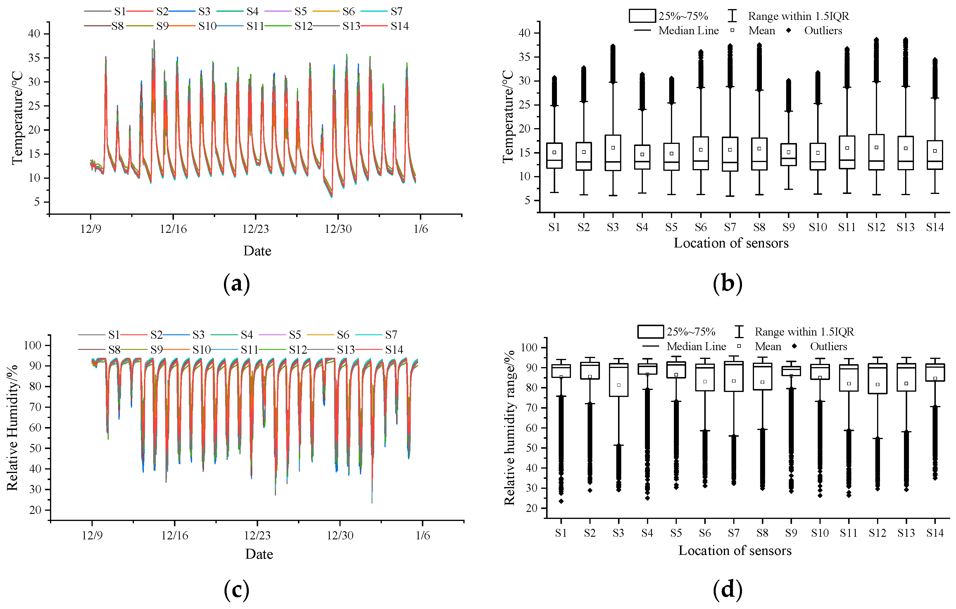
3.1.1. Temperature and Humidity Heterogeneity in the North–South Vertical Direction

Through the analysis of 14 × 7880 sets of temperature and humidity data measured by 14 THSs in the north–south vertical direction, it was found that the temperature and humidity at different sites had the same trend with time but showed obvious spatial differences. The maximum temperature difference at the same time could be more than 6 °C, and the standard deviation of temperature data could be more than 2 °C, as shown in Figure 3a. Similarly, the maximum difference and standard deviation of relative humidity data could be more than 15% and 7%, respectively, as in Figure 3c. To quantitatively represent the spatial heterogeneity of temperature and humidity, the coefficient of variation (CV) is used as a characteristic index. As is well known, when the CV tends towards 0, the uniformity becomes better; when it tends towards 1, the uniformity becomes worse.

The temperature and humidity inside the CSG vary under the influence of solar radiation, ventilation, physiological activities of the crop, etc. Therefore, the heterogeneity of temperature and humidity also varies with time. Based on statistical data, the mean and median temperature CVs are both over 8.2%, and the mean and median relative humidity CVs are both over 9.8%. Meanwhile, during the dynamics of the CSG microclimate, the maximum CVs of temperature and relative humidity could reach 20.7% and 29.5%, respectively, indicating that there is obvious spatial heterogeneity of temperature and humidity along the vertical direction. This is because warm air heated by solar radiation is driven vertically upwards by the thermal buoyancy, resulting in higher temperature in the upper part of the CSG. At the same time, crop transpiration and soil evaporation generate large amounts of water vapor near the ground surface, resulting in higher humidity in the lower part.

In addition, from Figure 3b,d, the acquired temperature and humidity data contained many outliers, and the temperature outliers are all high-end values that appeared at noon, while the humidity outliers are all low-end values at the same time, indicating that the microclimate variation fluctuates more when the solar radiation is high.

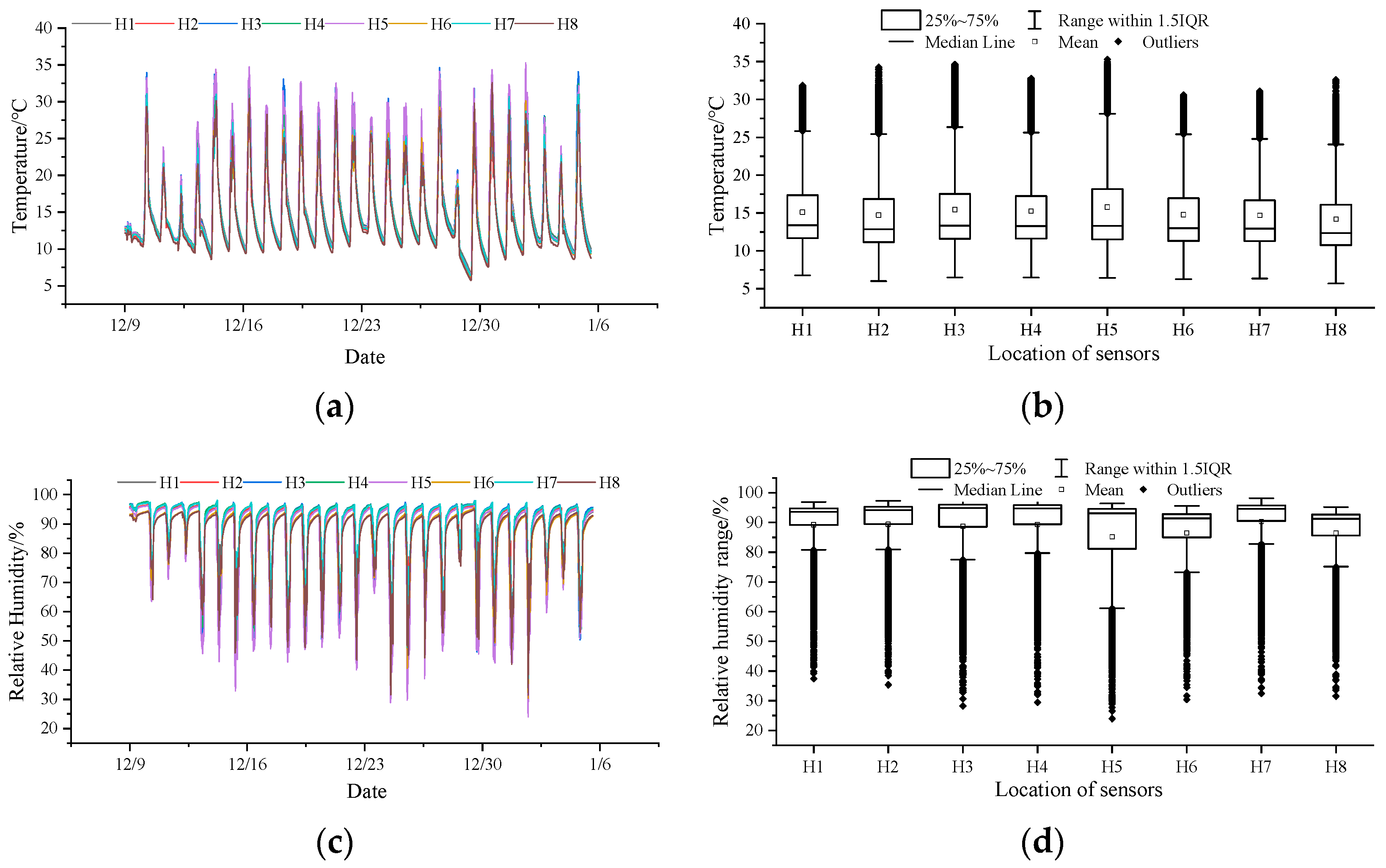
3.1.2. Temperature and Humidity Heterogeneity in the East–West Horizontal Direction

Through the analysis of 8 × 7880 sets of temperature and humidity data measured by eight THSs in the east–west horizontal direction, it was found that the temperature and humidity in the horizontal direction had similar temporal periodicity and spatial variability as that in the vertical direction. The maximum CVs of temperature and relative humidity could reach 12.9% and 17.1%, respectively, and the maximum temperature and relative humidity differences could reach 3.3 °C and 15%, respectively, as in Figure 4a,c. In addition, similar to Figure 3b,d, we can also find many outliers in Figure 4b,d, whose appearance also occurs during the time period of highest solar radiation intensity, suggesting that temperature and humidity fluctuate more dramatically around noon. Therefore, if we want to comprehensively monitor CSG microclimate, the horizontal heterogeneity should not be ignored either.

The above analysis revealed the spatial heterogeneity of the CSG microclimate, so it is necessary to use multiple THSs to comprehensively reflect the spatial distribution of temperature and humidity. Meanwhile, considering the spatial correlation of temperature and humidity in neighboring locations, there is information redundancy in neighboring THSs. Therefore, it provides optimization potential for THS configuration with the aim of reducing the number of THSs and saving costs.

3.2. Optimization Results of THS Configuration

3.2.1. Priority Ranking for the THSs

Based on the priority ranking strategy in Section 2.3.2, the priority ranking results of the 14 THSs in the vertical direction and the 8 THSs in the horizontal direction can be determined, respectively, as shown in

Table 1. THS ranking in the vertical direction.

THS Rank	THS Location	IIC	THS Rank	THS Location	IIC
1	S6	570	8	S10	537
2	S9	449	9	S7	541
3	S8	512	10	S1	539
4	S4	505	11	S5	549
5	S3	518	12	S13	550
6	S2	523	13	S12	560
7	S14	530	14	S11	566

and

Table 2. THS ranking in the horizontal direction.

THS Rank	THS Location	IIC	THS Rank	THS Location	IIC
1	H6	550	5	H3	525
2	H5	523	6	H1	527
3	H2	506	7	H8	533
4	H7	526	8	H4	535

.

3.2.2. Determination of THS Quantity Required

As shown in Figure 5, the RMSE showed a decreasing trend as the number of THSs selected increased. At the same time, the IGR introduced by new THSs also showed a decreasing trend, as shown in Figure 6, which indicates that the information gain contributed by newly added THSs is very limited when the number of THSs exceeds a certain quantity. The specific THSs could then be selected according to different cost budgets and accuracy requirements. Two configuration scenarios are presented here as the examples: low monitoring requirement with a low cost budget; high monitoring requirement with a high cost budget.

(1)

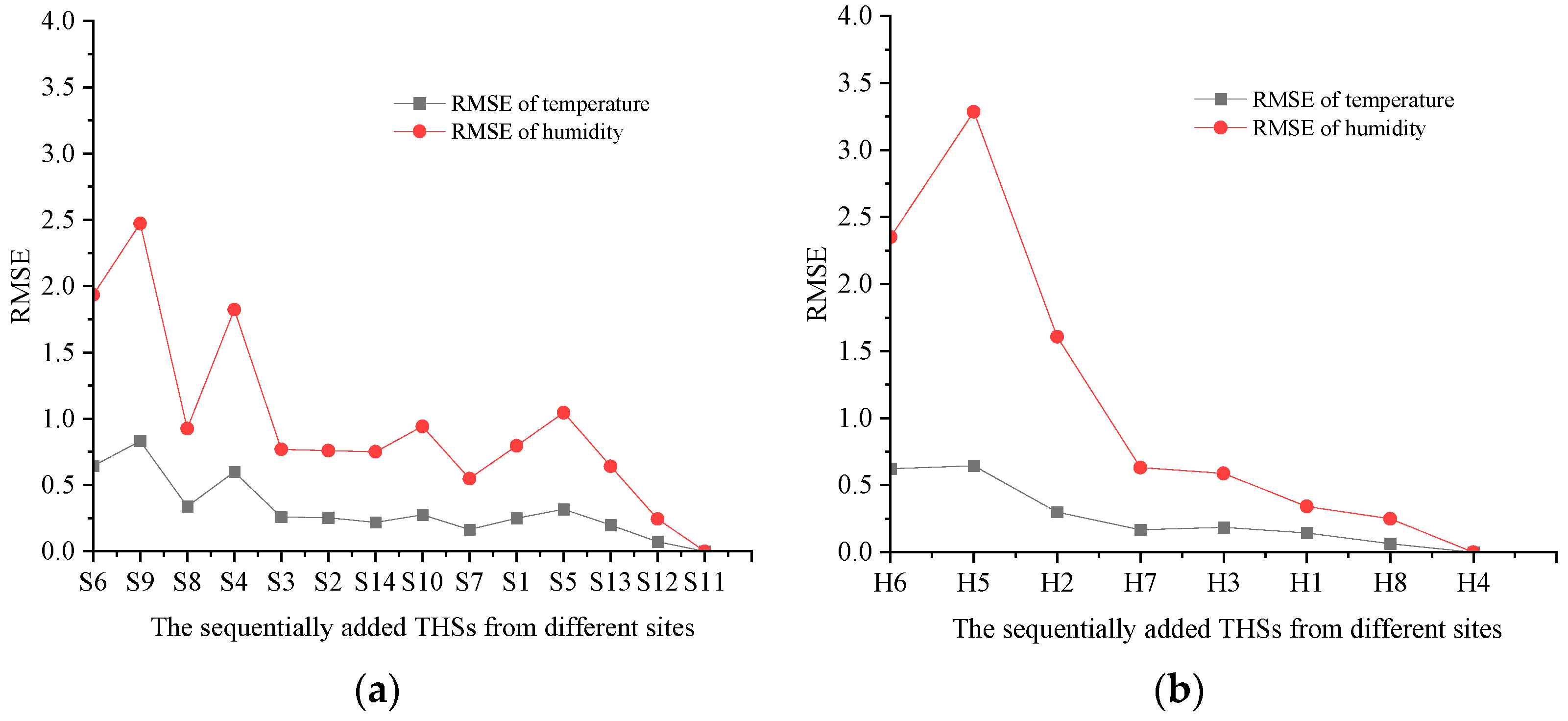
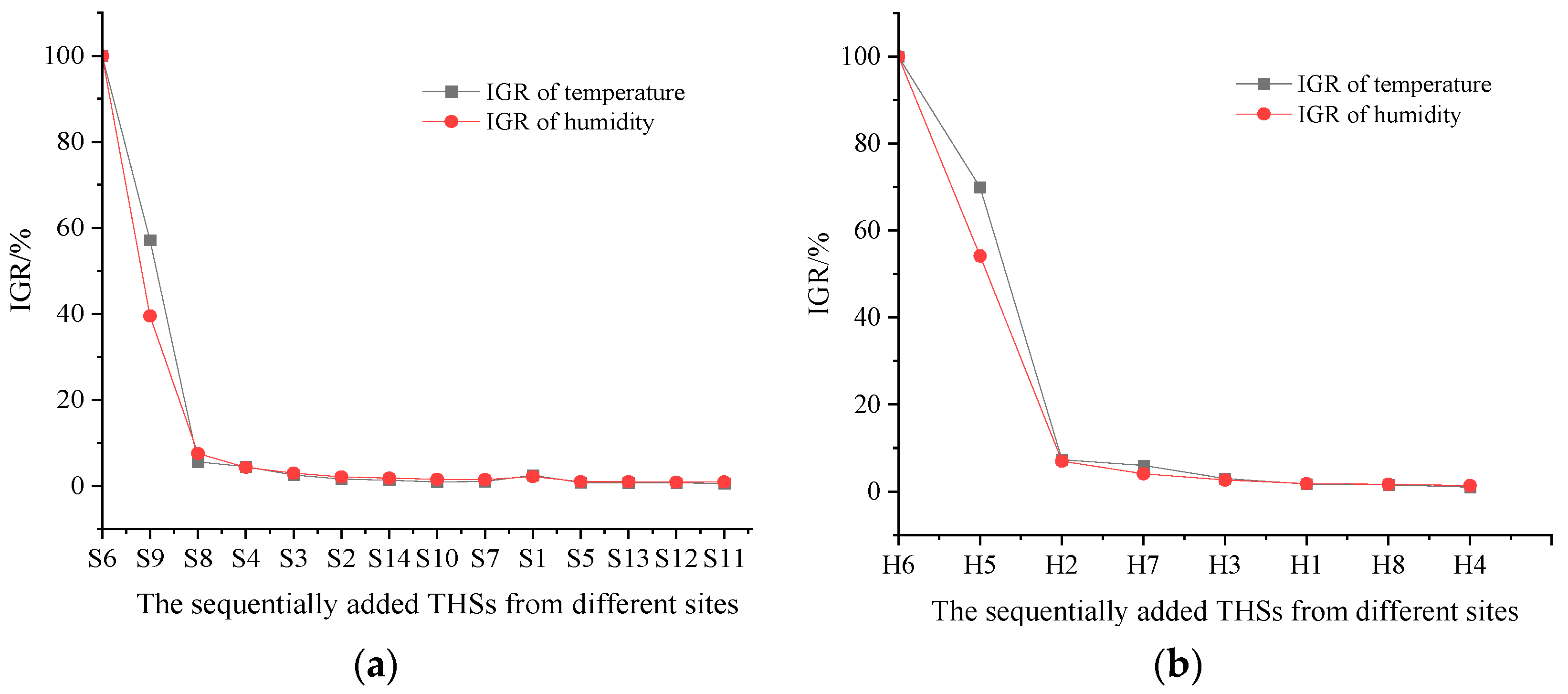
Low monitoring requirement scenario under low cost budget: For illustration, the RMSE thresholds for temperature and relative humidity are set to 1 °C and 10%, respectively, and the IGR threshold is set to 10%. As in Figure 5a, the RMSE of temperature and relative humidity are 0.64 °C and 1.9%, respectively, with the first ranked THS S6 in the vertical direction, which meets the temperature- and humidity-monitoring requirement. However, THS S6 cannot meet the IGR requirement by itself, so the second ranked THS S9 is also needed to improve the information abundance. From Figure 6a, the temperature IGR and relative humidity IGR of the next THS are 5.5% and 7.5%, respectively, both of which meet the IGR threshold of 10%. Therefore, in this scenario, two THSs, S6 and S9, are selected in the vertical direction to meet the dual requirements of monitoring accuracy and information abundance, i.e., $n_{\mathrm{vertical}}=2$.

Similarly, according to the RMSE threshold, the first ranked THS H6 in the horizontal direction could meet the monitoring accuracy requirements, whose RMSEs of temperature and relative humidity are 0.62 °C and 2.4%, respectively. In addition, the THS H6 alone cannot meet the IGR requirement, so the second ranked THS H5 must be selected. Then, the temperature IGR and relative humidity IGR of the next THS are 7.3% and 7.0%, respectively, meeting the IGR requirement of 10%. Therefore, in this scenario, two THSs, H6 and H5, should be selected in the horizontal direction, i.e., $n_{\mathrm{horizontal}}=2$.

(2)

Scenario with high monitoring requirement under high cost budget: When the monitoring requirements of temperature and humidity are high, the cost budget should be correspondingly improved. Then, the RMSE thresholds of temperature and relative humidity are set at 0.5 °C and 5%, respectively, and the IGR threshold is set at 7%. In this scenario, as in Figure 5a, when the THS number is increased to three in the vertical direction, the RMSEs of temperature and relative humidity are 0.34 °C and 0.92%, respectively, which both meet the RMSE thresholds. Meanwhile, the temperature IGR and the relative humidity IGR of the next THS are 4.4% and 4.3%, respectively, both below the threshold value of 7%. In summary, to meet the strict requirements of monitoring accuracy and information abundance, the top three THSs in the vertical direction should be selected, i.e., $n_{\mathrm{vertical}}=3$.

Similarly, when the number of THSs in the horizontal direction is increased to three, the RMSEs of temperature and relative humidity are 0.30 °C and 2.4%, respectively, and the IGRs of temperature and relative humidity are 5.9% and 4.1%, respectively, which meet the monitoring requirement. Therefore, in order to meet the high requirements of monitoring accuracy and information abundance, the top three THSs in the horizontal direction should be selected, i.e., $n_{\mathrm{horizontal}}=3$.

3.2.3. Optimal Configuration of the THSs Required

Based on the above analysis, in the case of a low cost budget, the number of THSs is set to two in both the vertical and the horizontal directions. According to the priority ranking results, the specific THSs S6 and S9 in the vertical direction and H6 and H5 in the horizontal direction could meet the dual objectives of cost constraint and monitoring requirement; in the case of a high monitoring requirement, additional THSs S8 and H2 should be added in the vertical and horizontal directions, respectively, to improve the monitoring accuracy and information abundance of the CSG monitoring, summarized in

Table 3. Optimal THS configuration in the CSG.

Monitoring Orientation	Low Cost Budget	High Monitoring Requirement
The vertical direction	S6, S9	S6, S9, S8
The horizontal direction	H6, H5	H6, H5, H2

.

3.2.4. Validation of the Optimal Configuration Strategy

(1)

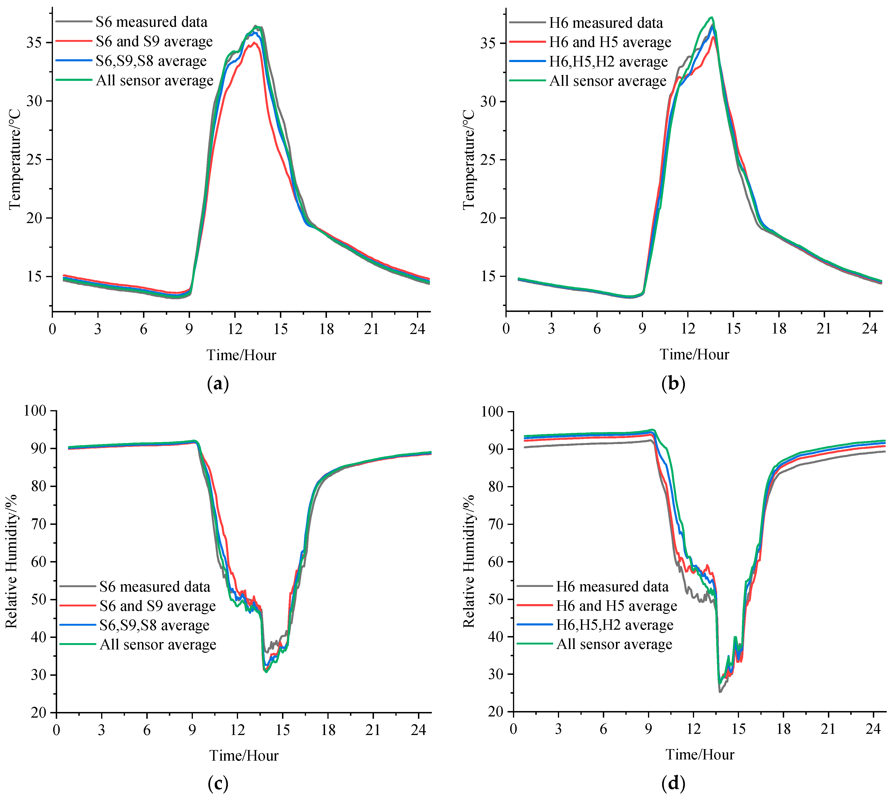
Characterization performance

To verify the effectiveness of the proposed strategy, the monitoring RMSE and IGR of the THS configuration produced according to the strategy were compared with those of all the THSs, as shown in Figure 7 and

Table 4. Validation results of THS configurations.

THS Configuration	Temperature RMSE (°C)	Relative Humidity RMSE (%)	Temperature IGR (%)	Relative Humidity IGR (%)
S6, S9 #	0.60	1.32	6.70	10.0
H6, H5 #	0.50	2.30	9.47	9.1
S6, S9, S8 #	0.23	0.58	4.80	8.7
H6, H5, H2 #	0.33	1.10	6.90	6.0
S6, S2 *	0.62	1.8	13.5	21.5
S5, S2 *	0.51	1.9	14.3	21.1
H1, H2 *	0.46	1.35	12.8	20.2
H7, H3 *	0.47	1.64	11.3	20.8
S6 S2 S14 *	0.30	1.2	8.3	14.6
S5 S2 S11 *	0.43	1.48	8.7	15.0
H1 H2 H4 *	0.3	0.86	8.7	14.2
H7 H3 H8 *	0.33	0.85	7.2	13.2

Note: # represents the optimized configuration; * represents the randomly composed ones.

. For both the THS configuration with low cost budget and that with high monitoring requirement, the temperature and humidity curves of the selected THSs are in good agreement with those of all THSs, as in Figure 7. For the THS configuration with low cost budget, the RMSE and IGR of temperature and relative humidity are all below the thresholds (RMSE: 1 °C and 10%; IGR: both 10%), thus satisfying the dual requirements of monitoring accuracy and information abundance. If the monitoring requirements are higher, additional THSs S8 and H2 will be added to the monitoring configuration, further reducing the RMSE and IGR. The comparison showed that the optimized monitoring configuration with only four or six THSs could accurately and comprehensively monitor the CSG microclimate with good characterization performance. The proposed strategy could significantly reduce THS usage and save monitoring investment.

(2)

Comparative advantage

To validate the comparative advantage of the optimized monitoring configurations, the RMSE and IGR of eight randomly composed THS configurations were calculated, also in Table 4. The number of THSs in the eight configurations is the same as in the optimized configurations. Of the 16 monitoring RMSE values of the random configurations, 11 values were larger than those of the optimized configurations, indicating that the optimized configurations have the better monitoring accuracy. Furthermore, the IGR values of the random configurations are about twice those of the optimized ones, showing that the optimized configurations could comprehensively monitor the CSG microclimate much better.

3.3. Discussion

Compared to the single-point monitoring method, the proposed configuration strategy could reflect the spatial heterogeneity of the CSG microclimate with a few THSs. It is cost-effective to achieve accurate and comprehensive microclimate monitoring with a small increase in investment. Compared with the uniform multi-point monitoring method [7,8], the proposed strategy could significantly reduce the use of THSs and save investment, while maintaining monitoring accuracy and comprehensiveness within acceptable error. Taking the test CSG in this paper as an example, we used only four or six THSs to achieve accurate and comprehensive monitoring. Compared to the original monitoring configuration with 22 THSs, the proposed strategy could achieve a 72.7~81.8% reduction in THS usage. It indicates that the proposed strategy has the potential to provide efficient and cost-effective monitoring solutions for cost-sensitive CSGs.

Moreover, there are some necessary works in future study to further improve the effectiveness and universality of the proposed strategy. The optimal configuration strategy was constructed based on the spatial heterogeneity of the CSG microclimate, without considering the temporal variety of the microclimate. In practice, the temporal diversity interacts with the spatial distribution. As shown in Section 3.1, the spatial heterogeneity during the night is much less than that during the daytime. To further improve the adaptability and effectiveness of the proposed strategy, it is essential to integrate the effects of spatial distribution and temporal variety of the microclimate. Meanwhile, the proposed strategy has only been validated with the test data collected from a tomato CSG. There are differences in the morphological characteristics and physiological activities of different crops. The tomato crop does not adequately represent the effects of different crops on the CSG microclimate. We plan to verify and improve the universality of the strategy using the microclimate data sampled from CSGs with other crops, such as cucumber, eggplant, and lettuce.

4. Conclusions

In order to accurately monitor the CSG microclimate under cost constraints, an optimal THS configuration strategy was proposed based on the improved weighted HSIC. The selection priority of all the THSs was ranked based on the relative independence values, which were calculated according to the improved HSIC matrix. To simultaneously meet the monitoring requirement and the cost constraint, the appropriate number of THSs would be selected sequentially to form the suitable monitoring solution. Under strict cost constraints, the monitoring solution with four THSs (S6, S9 and H6, H5) was constructed based on the proposed strategy, with the maximum RMSE of 2.3%, 0.6 °C and the maximum IGR of 9.47%, 10% for temperature and relative humidity, respectively. For a higher monitoring requirement, additional THSs S8, H2 should be added to the solution, further reducing the monitoring RMSE and IGR. The proposed strategy could significantly reduce THS usage and save investment, while maintaining the monitoring accuracy and comprehensiveness. It could provide a theoretical reference and cost-effective solution for CSG microclimate monitoring.

References

1. Liu, X.; Wu, X.; Xia, T.; Fan, Z.; Shi, W.; Li, Y.; Li, T. New Insights of Designing Thermal Insulation and Heat Storage of Chinese Solar Greenhouse in High Latitudes and Cold Regions. Energy 2022, 242, 122953. [Google Scholar] [CrossRef]
2. Vanthoor, B.H.E. A Model-Based Greenhouse Design Method; Wageningen University: Wageningen, The Netherlands, 2011. [Google Scholar]
3. Zou, W.; Zhang, B.; Yao, F.; He, C. Verification and forecasting of temperature and humidity in solar greenhouse based on improved extreme learning machine algorithm. Trans. Chin. Soc. Agric. 2015, 31, 194–200. [Google Scholar]
4. Ferentinos, K.P.; Katsoulas, N.; Tzounis, A.; Bartzanas, T.; Kittas, C. Wireless Sensor Networks for Greenhouse Climate and Plant Condition Assessment. Biosyst. Eng. 2017, 153, 70–81. [Google Scholar] [CrossRef]
5. Jiang, G.; Hu, Y.; Liu, Y.; Zou, Z. Analysis on insulation performance of sunken solar greenhouse based on CFD. Trans. Chin. Soc. Agric. Eng. 2011, 27, 275–281, (In Chinese with English abstract). [Google Scholar]
6. Li, Z.; Wang, T.; Gong, Z.; Li, N. Forewarning technology and application for monitoring low temperature disaster in solar greenhouses based on internet of things. Trans. Chin. Soc. Agric. Eng. 2013, 29, 229–236, (In Chinese with English abstract). [Google Scholar]
7. Zong, Z. Study on Monitoring System of Greenhouse Group and the Spatial and Temporal Distribution of the Environmental Parameters; Inner Mongolia Agricultural University: Hohhot, China, 2018; (In Chinese with English abstract). [Google Scholar]
8. Wang, T.; Dai, X.; Liu, Y. Learning with Hilbert–Schmidt Independence Criterion: A Review and New Perspectives. Knowl.-Based Syst. 2021, 234, 107567. [Google Scholar] [CrossRef]
9. Mancuso, M.; Bustaffa, F. A Wireless Sensors Network for Monitoring Environmental Variables in a Tomato Greenhouse. In Proceedings of the 2006 IEEE International Workshop on Factory Communication Systems, Torino, Italy, 27–30 June 2006; pp. 107–110. [Google Scholar]
10. Lu, X.; Ding, Y.; Hao, K. Adaptive Design Optimization of Wireless Sensor Networks Using Artificial Immune Algorithms. In Proceedings of the 2008 IEEE Congress on Evolutionary Computation (IEEE World Congress on Computational Intelligence), Hong Kong, China, 1–6 June 2008; pp. 788–792. [Google Scholar]
11. Feng, L.; Li, H.; Zhi, Y. Greenhouse CFD Simulation for Searching the Sensors Optimal Placements. In Proceedings of the 2013 Second International Conference on Agro-Geoinformatics (Agro-Geoinformatics), Fairfax, VA, USA, 12–16 August 2013; pp. 504–507. [Google Scholar]
12. Cheng, X.; Li, D.; Shao, L.; Ren, Z. A Virtual Sensor Simulation System of a Flower Greenhouse Coupled with a New Temperature Microclimate Model Using Three-Dimensional CFD. Comput. Electron. Agric. 2021, 181, 105934. [Google Scholar] [CrossRef]
13. Ali, A.; Hassanein, H.S. Optimal Placement of Camera Wireless Sensors in Greenhouses. In Proceedings of the ICC 2021—IEEE International Conference on Communications, Montreal, QC, Canada, 14–23 June 2021; pp. 1–6. [Google Scholar]
14. Sharma, H.; Vaidya, U.; Ganapathysubramanian, B. A Transfer Operator Methodology for Optimal Sensor Placement Accounting for Uncertainty. Build. Environ. 2019, 155, 334–349. [Google Scholar] [CrossRef]
15. Dur, T.H.; Arcucci, R.; Mottet, L.; Solana, M.M.; Pain, C.; Guo, Y.-K. Weak Constraint Gaussian Processes for Optimal Sensor Placement. J. Comput. Sci. 2020, 42, 101110. [Google Scholar] [CrossRef]
16. Löhner, R.; Camelli, F. Optimal Placement of Sensors for Contaminant Detection Based on Detailed 3D CFD Simulations. Eng. Comput. 2005, 22, 260–273. [Google Scholar] [CrossRef]
17. Arnesano, M.; Revel, G.M.; Seri, F. A Tool for the Optimal Sensor Placement to Optimize Temperature Monitoring in Large Sports Spaces. Autom. Constr. 2016, 68, 223–234. [Google Scholar] [CrossRef]
18. Suryanarayana, G.; Arroyo, J.; Helsen, L.; Lago, J. A Data Driven Method for Optimal Sensor Placement in Multi-Zone Buildings. Energy Build. 2021, 243, 110956. [Google Scholar] [CrossRef]
19. Cheng, J.C.P.; Kwok, H.H.L.; Li, A.T.Y.; Tong, J.C.K.; Lau, A.K.H. BIM-Supported Sensor Placement Optimization Based on Genetic Algorithm for Multi-Zone Thermal Comfort and IAQ Monitoring. Build. Environ. 2022, 216, 108997. [Google Scholar] [CrossRef]
20. Lee, S.; Lee, I.; Yeo, U.; Kim, R.; Kim, J. Optimal Sensor Placement for Monitoring and Controlling Greenhouse Internal Environments. Biosyst. Eng. 2019, 188, 190–206. [Google Scholar] [CrossRef]
21. Gretton, A.; Bousquet, O.; Smola, A.; Schölkopf, B. Measuring Statistical Dependence with Hilbert-Schmidt Norms. In Algorithmic Learning Theory; Jain, S., Simon, H.U., Tomita, E., Eds.; Lecture Notes in Computer Science; Springer: Berlin/Heidelberg, Germany, 2005; Volume 3734, pp. 63–77. ISBN 978-3-540-29242-5. [Google Scholar]
22. Feng, L.; Di, T.; Zhang, Y. HSIC-Based Kernel Independent Component Analysis for Fault Monitoring. Chemom. Intell. Lab. Syst. 2018, 178, 47–55. [Google Scholar] [CrossRef]
23. Rustamov, R.M.; Klosowski, J.T. Kernel Mean Embedding Based Hypothesis Tests for Comparing Spatial Point Patterns. Spat. Stat. 2020, 38, 100459. [Google Scholar] [CrossRef]
24. Vitetta, G.M.; Taylor, D.P.; Colavolpe, G.; Pancaldi, F.; Martin, P.A. Elements of Information Theory; John Wiley & Sons, Ltd.: Hoboken, NJ, USA, 2013; ISBN 978-1-118-57661-8. [Google Scholar]
25. Pei, X.-Y.; Yi, T.-H.; Qu, C.-X.; Li, H.-N. Conditional Information Entropy Based Sensor Placement Method Considering Separated Model Error and Measurement Noise. J. Sound Vib. 2019, 449, 389–404. [Google Scholar] [CrossRef]
26. Zhang, J.; Lin, Z.; Tsai, P.-W.; Xu, L. Entropy-Driven Data Aggregation Method for Energy-Efficient Wireless Sensor Networks. Inf. Fusion 2020, 56, 103–113. [Google Scholar] [CrossRef]
27. Wang, X.; Ma, J.; Wang, S. Parallel Energy-Efficient Coverage Optimization with Maximum Entropy Clustering in Wireless Sensor Networks. J. Parallel Distrib. Comput. 2009, 69, 838–847. [Google Scholar] [CrossRef]
Figure 1. Temperature- and humidity-monitoring system in the CSG. (a) Temperature and humidity data collected with IoT platform; (b) THS spatial layout diagram. Note: S1~S14 and H1~H8 represent the sensors located in north–south vertical direction and in east–west horizontal direction, respectively.
Agriculture 14 00311 g001
Figure 2. Flow chart of THS configuration optimization.
Agriculture 14 00311 g002
Figure 3. Temperature and humidity in the north–south vertical direction (9 December–6 January). (a) Temperature in the vertical direction; (b) Box chart of temperature in the vertical direction; (c) Relative humidity in the vertical direction; (d) Box chart of relative humidity in the vertical direction.
Agriculture 14 00311 g003
Figure 4. Temperature and humidity in the east–west horizontal direction (9 December–6 January). (a) Temperature in the horizontal direction; (b) Box chart of temperature in the horizontal direction; (c) Relative humidity in the horizontal direction; (d) Box chart of relative humidity in the horizontal direction.
Agriculture 14 00311 g004
Figure 5. The RMSE curve of temperature and humidity with the increase in THS quantity. (a) RMSE variation with the increase in THS quantity in vertical direction; (b) RMSE variation with the increase in THS quantity in horizontal direction.
Agriculture 14 00311 g005
Figure 6. The IGR curve of temperature and humidity with the increase in THS quantity. (a) IGR variation with the increase in THS quantity in vertical direction; (b) IGR variation with the increase in THS quantity in horizontal direction.
Agriculture 14 00311 g006
Figure 7. The temperature and relative humidity curves with different THS combinations (12 January). (a) The temperature curves in the vertical direction; (b) The relative humidity curves in the vertical direction; (c) The temperature curves in the horizontal direction; (d) The relative humidity curves in the horizontal direction.
Agriculture 14 00311 g007