Research on the Identification Method of Maize Seed Origin Using NIR Spectroscopy and GAF-VGGNet

Abstract

The origin of seeds is a crucial environmental factor that significantly impacts crop production. Accurate identification of seed origin holds immense importance for ensuring traceability in the seed industry. Currently, traditional methods used for identifying the origin of maize seeds involve mineral element analysis and isotope fingerprinting, which are laborious, destructive, time-consuming, and suffer from various limitations. In this experiment, near-infrared spectroscopy was employed to collect 1360 maize seeds belonging to 12 different varieties from 8 distinct origins. Spectral information within the range of 11,550–3950 cm⁻¹ was analyzed while eliminating multiple interferences through first-order derivative combined with standard normal transform (SNV). The processed one-dimensional spectral data were then transformed into three-dimensional spectral maps using Gram’s Angle Field (GAF) to be used as input values along with the VGG-19 network model. Additionally, a convolution layer with a step size of 1 × 1 and the padding value set at 1 was added, while pooling layers had a step size of 2 × 2. A batch size of 48 and learning rate set at 10⁻⁸ were utilized while incorporating the Dropout mechanism to prevent model overfitting. This resulted in the construction of the GAF-VGG network model which successfully decoded the output into accurate place-of-origin labels for maize seed detection. The findings suggest that the GAF-VGG network model exhibits significantly superior performance compared to both the original data and the PCA-based origin identification model in terms of accuracy, recall, specificity, and precision (96.81%, 97.23%, 95.35%, and 95.12%, respectively). The GAF-VGGNet model effectively captures the NIR features of different origins of maize seeds without requiring feature wavelength extraction, thereby reducing training time and enhancing accuracy in identifying maize seed origin. Moreover, it simplifies near-infrared (NIR) spectral modeling complexity and presents a novel approach to maize seed origin identification and traceability analysis.

1. Introduction

Seed origin is a critical factor that influences crop production [1], and the traceability of agricultural products’ origins holds significant importance for ensuring food security [2]. The origin of maize seeds plays a pivotal role in determining both yield and quality, serving as a fundamental basis for acquiring and grading maize, as well as establishing a robust traceability system [3]. Therefore, the detection of maize seed origin carries substantial research value.

Traditional sensory analysis methods primarily focus on grain weight, grain thickness, volume, density, color, gloss, and other phenotypic traits [4]. However, these parameters heavily rely on subjective human experience and have relatively high technical requirements, leading to low detection efficiency [5]. Consequently, the conclusive identification of maize seed origin remains challenging. Currently, mineral element analysis [6] and isotope fingerprinting [7], combined with chemometrics for precise origin identification, are predominantly employed. Nevertheless, these approaches are not suitable for maize seed origin identification due to their cumbersome and destructive procedures as well as time-consuming nature.

In recent years, NIR spectroscopy has garnered significant attention from numerous research teams due to its rapid, non-destructive, and environmentally friendly characteristics in the identification of crop varieties and origins [8]. Shekh et al. [9] established NIR spectroscopy datasets for various parts of maize and trained them using a one-dimensional convolutional neural network (1D-CNN), partial least squares regression (PLSR), and artificial neural network to differentiate between different maize varieties. Arena et al. [10] analyzed the fatty acids in pistachio seeds using near-infrared spectroscopy and successfully distinguished their origins by combining multivariate analysis techniques. Salles et al. [11] employed near-infrared spectroscopy combined with principal component analysis (PCA) to identify key markers for the origin determination of guarana seeds. Zheng et al. [12] collected and analyzed NIR spectra from apple samples of varying sizes and detection positions, selecting effective wavelengths through a variable size moving window method and competitive adaptive weighted sampling technique before constructing a 1D-CNN model. The results demonstrated that the constructed 1D-CNN model was more accurate than the PLSR method, providing a convenient alternative for online soluble solids determination in apples while significantly reducing complexity in the NIR spectral modeling process. Vitale et al. [13] employed NIR spectroscopy in conjunction with chemometrics to discern the geographical origin of pistachios from six distinct regions, namely, Sicily, India, Iran, Syria, Turkey, and the USA. The SIMCA and PLS-DA methods were utilized for classification purposes. The findings revealed that both classification models developed using these methods exhibited an accuracy rate exceeding 90%, thereby demonstrating the efficacy of integrating NIR spectroscopy and chemometric classification techniques as a valuable tool for tracing the provenance of pistachios. However, when analyzing NIR spectra, it is often necessary to extract the characteristic wavelengths. The extracted feature data are susceptible to interference during the extraction process and, as a result, deep learning models often face challenges in directly interpreting one-dimensional data.

In order to address the aforementioned issues, both domestic and foreign researchers and scholars have utilized the GAF advantage to enhance the effective information of one-dimensional data, optimize convolutional neural network performance, and ultimately improve discriminative model accuracy. The study conducted by Jin et al. [14] involved the conversion of Vis-NIR data into spectral images using GAF, which were then combined with the Swin Transformer model to successfully predict soil properties. The findings demonstrated that GAF effectively enhanced the performance of the deep learning model for spectral analysis. The study conducted by Li et al. [15] involved the encoding of one-dimensional spectra into two-dimensional images through the integration of visible–near-infrared (VNIR) spectroscopy with GAF. These encoded images were then inputted into the ConvNeXt V2-CAP model to enable the detection and classification of five different potato varieties. The findings demonstrated that utilizing GAF coding for spectral data significantly enhanced the accuracy of classification compared to directly employing a one-dimensional classification model. Tan et al. [16] introduced a rapid identification method for composite fertilizers using NIR spectroscopy in combination with GAF image coding and a quaternionic number convolutional neural network. The classification accuracy and adaptability of the proposed GAF-QCNN model are significantly enhanced compared to traditional methods such as principal component analysis combined with support vector machine classification, 1D convolutional neural networks, and partial least squares discriminant analysis.

When previous researchers utilized NIR spectra, they typically needed to extract the feature wavelengths of NIR spectra prior to employing machine learning methods or re-establishing 1D-CNN models. However, the extraction of feature wavelengths corresponding to the functional groups of their respective nutrients from NIR spectra was a laborious task. In contrast, the GAF method employed in this paper only necessitates converting the NIR spectra into images without requiring feature extraction. This approach enables a more intuitive analysis of the NIR spectral data and effectively resolves the issue of cumbersome feature wavelength extraction. The modeling process of NIR spectra is often excessively intricate and necessitates the re-establishment of 1D-CNN models tailored to specific problems. This paper integrates the GAF method with CNN, which has gained widespread usage in image analysis at this stage. By simply adjusting the input and specific parameters of the CNN network, it achieves superior results compared to traditional methods while reducing the complexity of NIR spectra modeling. Moreover, as data in a CNN network are represented as a three-dimensional matrix, training time can be minimized and training efficiency enhanced relative to 1D-CNN.

In this study, NIR spectroscopy was employed for the identification of maize seed origins. Maize seeds were selected as the subject of investigation, and the NIR data underwent preprocessing techniques such as first-order derivative derivation and SNV transformation to eliminate baseline drift and other background interferences. The one-dimensional spectra were then transformed into three-dimensional spectrograms using GAF for enhanced feature representation and convenient model input. Subsequently, a VGG model was utilized to extract features from the 3D spectral map in order to establish an origin identification model for maize seeds based on NIR and GAF-VGG. The objective is to develop a rapid method for identifying the origin of maize seeds while providing a novel approach towards establishing an origin identification and traceability system specifically designed for maize seeds.

2. Materials and Methods

2.1. Test Material

The maize seed samples, as depicted in Figure 1, were commercially acquired varieties. They were transported to the laboratory and placed in a controlled low-temperature and dry environment for preservation purposes. Defective seeds were excluded during the sample selection process, and the remaining samples were uniformly stored in glass containers. A total of 17 maize seed samples (variety codes A~L) from 12 distinct varieties were included, with 5 of them originating from 2 different sources. The product name is composed of the origin and variety of the sample. The origin code corresponds to the samples depicted in Figure 1, while detailed information regarding these samples is provided in

Table 1. Sample information.

Origin Labels	Code of Origin
Gansu Suke Sweet 1506	A1
Shandong Suke Sweet 1506	A2
Shanxi Hua Nuo 2	B1
Hebei Hua Nuo 2	B2
Shandong Star Sweet 230	C1
Beijing Star Sweet 230	C2
Shandong Moxidome	D1
Jiangsu Ink Pupil	D2
Xinjiang Tiangui Glutinous 932	E1
Guangxi Tiangui Glutinous 932	E2
Beijing Honey Blossom Sweet Glutinous 3	F
Beijing Star Sweet 221	G
Shandong Golden Sweet 13	H
Hebei Zhongnong Sweet 488	I
Shanxi Golden Queen	J
Shanxi Black Sticky 301	K
Gansu Huanai color sweet glutinous 102	L

The origin label comprises the geographical location of seed origin (front) and the specific variety (back). The original code corresponds to the map of maize seeds depicted in Figure 1.

.

2.2. Instruments and Equipment

The instrument utilized for the study is a TANGO model NIR spectrometer manufactured by Bruker, Germany (Saarbrücken, Germany), boasting a spectral resolution of 8 cm⁻¹. The instrument encompasses the NIR spectral range spanning from 870 nm to 2500 nm. The instrument was equipped with OPUS 6.5 software for spectral acquisition and Unscrambler X10.4 software from CAMO in Norway (Lysaker, Norway) for analysis purposes. Furthermore, a predictive model based on CNN was developed using Python version 3.8 (Amsterdam, The Netherlands) and the PyTorch framework (Berkeley, CA, USA).

2.3. Spectral Information Acquisition

The spectrometer was powered on and allowed to warm up for 30 min in order to acquire the background spectrum. To minimize the impact of light scattering and other undesirable factors caused by light passing through the bottom of the quartz cup during the spectral data collection of maize seeds, each prepared sample weighing 25 g was placed in a standard quartz cup with a volume of 0.3 dm³ for measurement. The samples were compressed using a sample presser to ensure consistent thickness and prevent visible light from penetrating through the bottom of the quartz cup. After each instrument scan, any remaining residue in the scanning cup was meticulously wiped clean to avoid cross-contamination between samples. Finally, each set of samples involved conducting 32 scans (repeated scanning to obtain an average value). During NIR spectrometer scanning, each labeled sample underwent 80 scans, resulting in a total of 1360 spectral data.

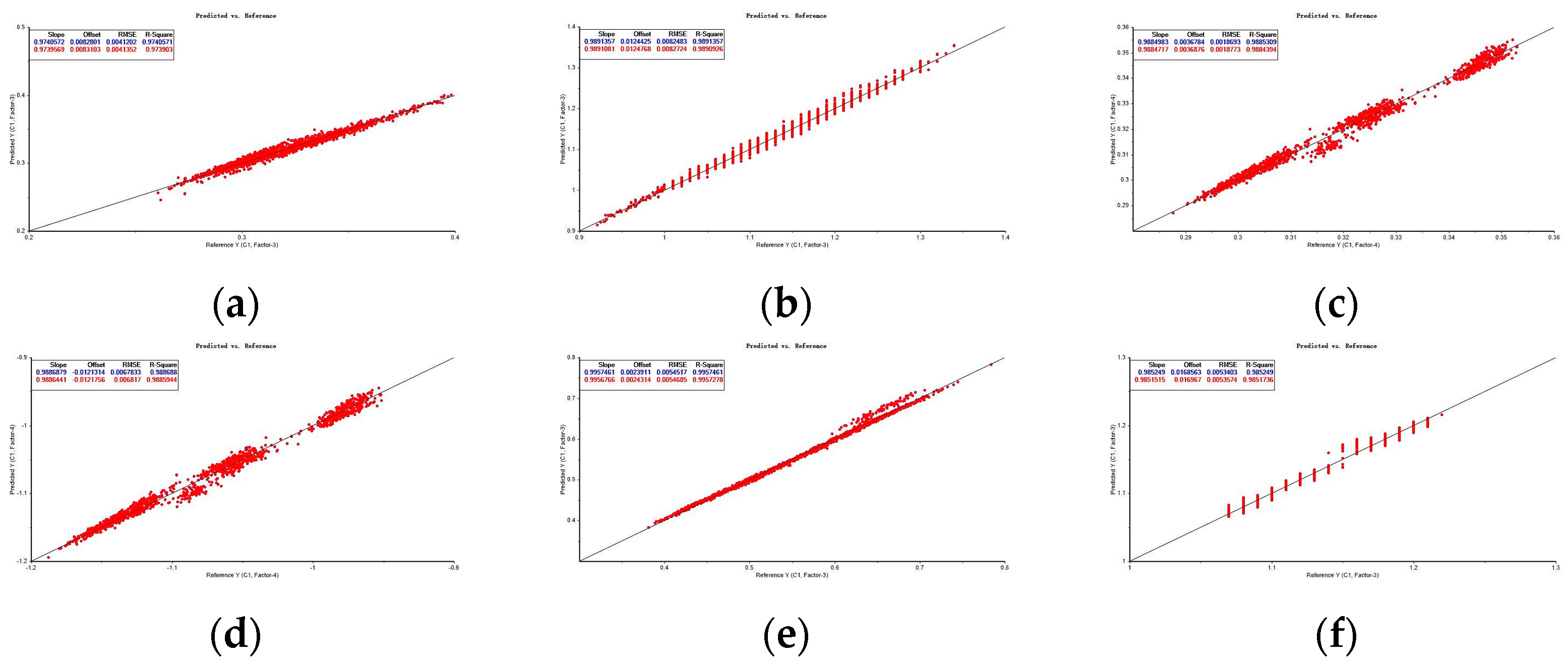
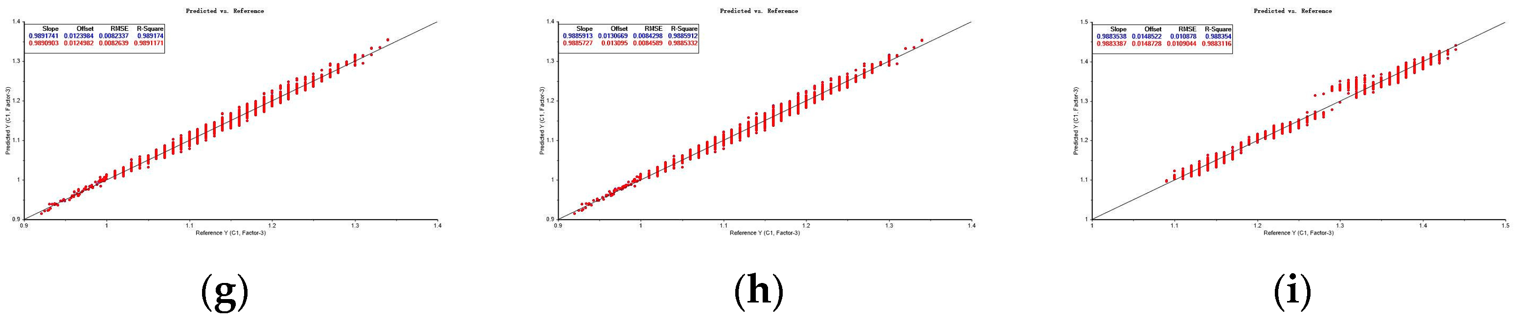
2.4. Spectral Preprocessing

Spectral signals in the near-infrared region are susceptible to environmental and instrumental interference, which can result in noisy spectral signals. The background spectra can also vary slightly after multiple acquisitions due to environmental changes, leading to baseline drift when the spectrometer makes successive acquisitions of the same type of seed. Correspondingly, noise in the spectra may appear due to other spectral interferences from the light source, thereby increasing the difficulty of analysis. Preprocessing is not only effective in minimizing noise interference but also enhances valid information from samples and strengthens the reliability of information contained in spectral data.

The original spectra of maize seeds were baseline corrected using first-order derivatives and combined with five preprocessing algorithms (CT, MSC, SNV, MA, and SG) to normalize, deflate, and transform the noise in the spectra. These algorithms also addressed issues related to light source scattering and normalization/deflation. The FD preprocessing technique not only eliminates background interference and baseline drift but also enhances the spectral resolution compared to the original spectrum [17]. CT preprocessing is a widely used data reconstruction method that effectively removes factors such as baseline shifts between samples and instrumental variations from the spectral data [18]. MSC preprocessing can be employed to eliminate noise caused by scattering issues in the spectra [19]. MA preprocessing effectively eliminates noise arising from time series, cyclic variations, and random fluctuations, enabling further analysis of data trends and the development direction [20]. SG preprocessing ensures the preservation of signal shape and width while filtering out unwanted noise components [21]. SNV preprocessing corrects spectral errors caused by scattering effects in measured sample spectra, thereby eliminating influences from changes in optical range or sample dilution on spectral response [22,23]. In practical spectrum analysis, multiple interferences are often encountered; therefore, combining various preprocessing methods helps mitigate these interferences for improved model accuracy and stability [24]. To evaluate the impact of these preprocessing algorithms (CT, MSC, SNV, MA, and SG), both the original spectral data and the data processed by these algorithms along with the first-order derivative algorithm were utilized to establish a PLSR model. The internal cross-validation correlation coefficients computed by this model (correlation coefficient ($R$), coefficient of determination ($R^2$), root mean squared error ($RMSE$), and standard error ($SE$)) were then employed as evaluation indices for assessing the effectiveness of preprocessing. This enabled us to select an optimal preprocessing method applicable to maize seed spectral data. The evaluation indices are presented in Equations (1)–(4).

$$R=\sqrt{1-\frac{\sum _{i=1}^n{({\widehat{y}}_i-y_i)}^2}{\sum _{i=1}^n{(y_i-\overline{y})}^2}},$$

(1)

$$R^2=\left(1-\frac{\sum {(y_{cv}-y)}^2}{\sum {(y_{cv}-\overline{y})}^2}\right)\times 100\mathrm{\%},$$

(2)

$$RMSE=\sqrt{\frac{\sum _{i=1}^n{(y_i-{\widehat{y}}_i)}^2}{n}},$$

(3)

$$SE=\sqrt{\frac{1}{M-1}\sum _{i=1}^M(a_i-b_i{)}^2},$$

(4)

where the measured and predicted values of the ith maize seed are $y_i$ and ${\widehat{y}}_i$, respectively, the mean of each measured value in the spectral value of maize seed is $\overline{y}$, and the correlation coefficients of the calibration set and the prediction set are $R_c$ and $R_p$, respectively. $y$ is the result of the measurement by the spectral data and the prediction by the mathematical model. $y_{cv}$ denotes the result of the determination by the standard method. $\overline{y}$ denotes the mean value of $y_{cv}.$ $a_i$ is the corresponding actual true value of the $i$th sample. $b_i$ is the calculated predicted value corresponding to the actual true value. $b_i$ is the calculated predicted value corresponding to the ith sample.

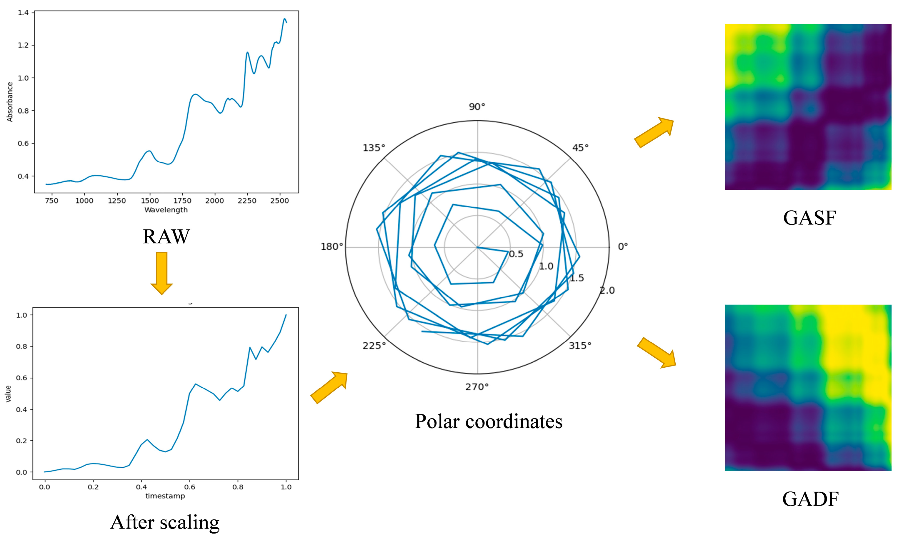
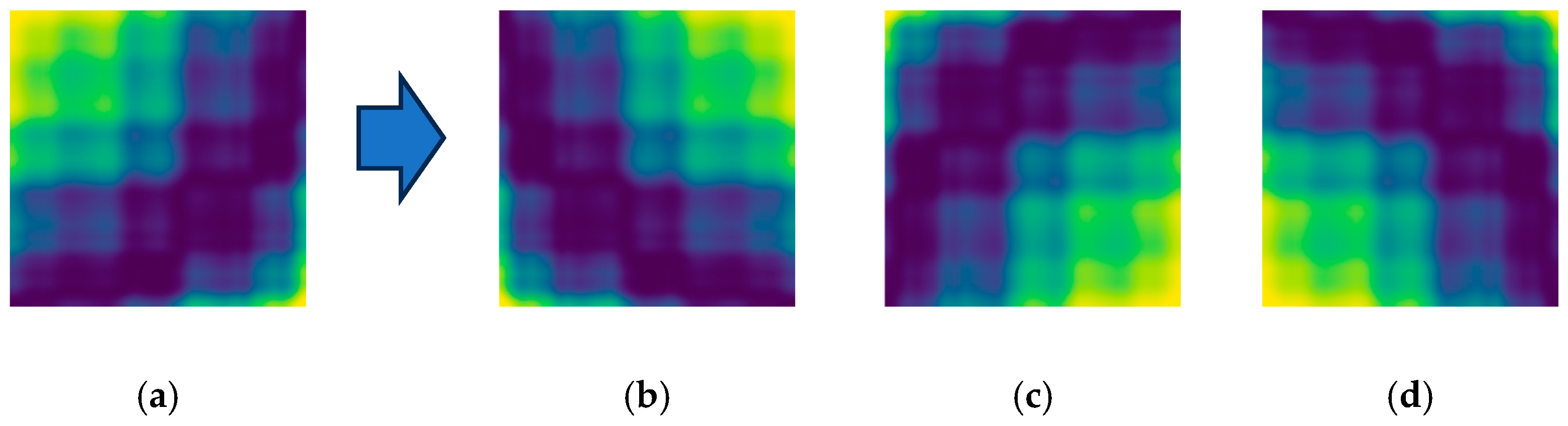
2.5. Near-Infrared Spectral Feature Map Conversion

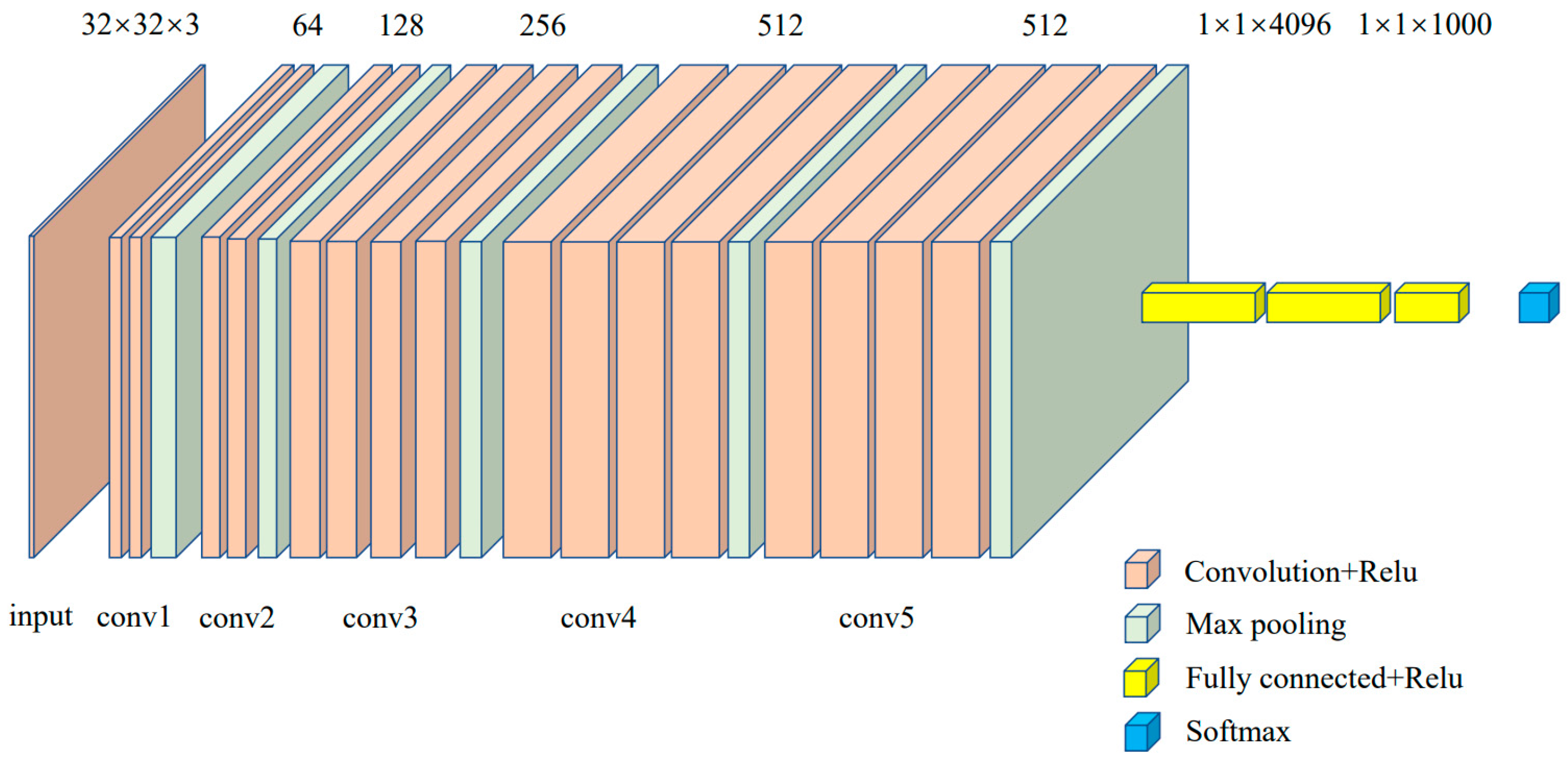
The NIR spectra are one-dimensional vectors that cannot be directly inputted into a neural network designed for three-dimensional matrices. Therefore, a specific one-dimensional convolutional neural network is required for model training. However, due to the large number of wavepoints (1845) in the original NIR spectra of maize seeds, each training iteration with the one-dimensional convolutional kernel contains less data, which can potentially result in slow network training. In contrast, three-dimensional images have the capability to comprehensively extract spectral information reflecting substances [25], offering advantages such as fast and accurate spectral information processing [26]. Considering these factors, this study employs GAF to transform the one-dimensional spectral data vector into a three-dimensional spectral information matrix in order to meet the requirements of the convolutional layer effectively. This approach fully harnesses the expressive ability of the model and applies it to research on maize seed origin identification methods.

GAF is an image decoding technique that transforms one-dimensional vectors into three-dimensional matrices by utilizing the Gram matrix to calculate the linear relationship between these vectors. It then encodes the temporal dependence of the time series into a two-dimensional image, ensuring its temporal coherence.

$$∆\left(a_1,a_2,\dots ,a_k\right)=\left(\begin{array}{cc}\begin{array}{cc}{(a}_1,a_1)& \left(a_1,a_2\right)\\ \left(a_2,a_1\right)& \left(a_2,a_2\right)\end{array}& \begin{array}{cc}\dots & \left(a_1,a_k\right)\\ \dots & \left(a_2,a_k\right)\end{array}\\ \begin{array}{cc}\dots & \dots \\ \left(a_k,a_1\right)& \left(a_k,a_2\right)\end{array}& \begin{array}{cc}\dots & \dots \dots \\ \dots & \left(a_k,a_k\right)\end{array}\end{array}\right)$$

(5)

In Equation (5), $a_1$ denotes the first point on the spectral data, $a_k$ denotes the last point on the spectral data, and the inner product of two by two between any $K$ vectors forms the Gram matrix.

The time series $X,$ given by the spectral signal, is first scaled to the interval [−1, 1] using Equation (6).

$${\tilde{x}}_i=\frac{\left[x_i-\mathit{max}\left(X\right)\right]+[x_i-min(X\left)\right]}{\mathit{max}\left(X\right)-min\left(X\right)}$$

(6)

In Equation (7), each corresponding value is encoded by a cosine value, and $t_i$ is encoded as a radius $r$, which is used to represent the time series $X$ in polar coordinates. The symbol ${\tilde{X}}_i$ denotes the element in the scaled time series $\tilde{X}$, while $t_i$ represents the corresponding timestamp. Additionally, $N$ signifies a constant that determines the span of the polar coordinate system.

$$\left\{\begin{array}{c}\phi =arccos\left({\tilde{x}}_i\right)\left(-1\le x_i\le 1,x_i\in \tilde{X}\right)\\ r=\frac{t_i}{N} (t\in \mathbb{N})\end{array}\right.$$

(7)

The cosine function $cos\left(\phi \right)$ exhibits monotonicity when $\phi \in [0, \pi ]$, given that $1 \le x_i \le 1$ and $0 \le {\phi }_i \le \pi$. Consequently, the polarized form establishes a bijective mapping with the time series $\tilde{X}$ itself, thereby establishing a unique relationship for encoding the time series in polar coordinates.

The deflated NIR spectral data are transformed into polar coordinates due to the varying angles of each data point. By employing Equations (8) and (9), the Gram angle sum field (GASF) and Gram angle difference field (GADF) can be derived through calculations involving sine function differences and cosine function sums for individual points. In this context, $G_s$ represents the GASF matrix, ${ G}_d$ represents the GADF matrix, I denotes the unit row vector, ${\tilde{X}}^{\prime }$ signifies the transpose vector of $\tilde{X}$, while $i$ and $j$ represent row and column indexes where $i$,$j \in N$ and $1 \le i$, $j \le n$.

$$G_S=\left[cos\left({\phi }_i+{\phi }_j\right)\right]={\tilde{X}}^{\prime }·\tilde{X}-{\sqrt{I-{\tilde{X}}^2}}^{\prime }·\sqrt{I-{\tilde{X}}^2},$$

(8)

$$G_d=\left[sin\left({\phi }_i-{\phi }_j\right)\right]={\sqrt{I-{\tilde{X}}^2}}^{\prime }·\tilde{X}-{\tilde{X}}^{\prime }·\sqrt{I-{\tilde{X}}^2}.$$

(9)

The equations above can be utilized to convert the given NIR spectral data into a feature matrix that is distributed along the diagonal, thereby encapsulating both raw values and angle information in a concise manner, which effectively represents the pertinent details of the NIR spectrum.

$$R_{\left(i,j\right)}=G_{\left(i,j\right)}=B_{\left(i,j\right)}=\frac{255}{G_{max}-G_{min}}-\left(G_{(i,j)}-G_{min}\right)$$

(10)

Finally, the individual elements of the matrix are rescaled to [0, 255] using Equation (10), which transforms the spectral information matrix into GAF. Subsequently, they are assigned to the R, G, and B channels for visualization as a standard RGB image. In this context, $R_{(i,j)}$, $G_{(i,j)}$, and $B_{(i,j)}$ denote the values of the three primary color channels in the image at position $(i,j)$. The schematic diagram illustrating Gram’s Angle Field encoding is presented in Figure 2. The colors depicted in the graph correspond to the pixel values, which span from 0 to 255.

2.6. Model Building

The data format of maize seed NIR spectra is transformed into 32 × 32 × 3 after GAF conversion. However, directly inputting it into the VGG-19 network after several rounds of convolution and pooling would result in a data size that is too small to complete the overall training process. To address this issue and enhance both accuracy and stability, optimization techniques are applied to the VGG-19 network. Given the initial image input’s small size, each convolution layer now includes a 1 × 1 stride and a 1 padding in addition to retaining the unique 3 × 3 convolution kernel of the VGG-19 network [27]. This ensures that the image size remains unchanged after each convolution while only modifying the number of input and output channels. Furthermore, during data dimensionality reduction, a unified 2 × 2 maximum pooling with an additional 2 × 2 stride is employed in order to maintain an image size of 32 × 32. Consequently, the improved VGGNet model comprises 16 convolutional layers, 3 fully connected layers, and utilizes a Softmax classifier for accurate classification prediction of specific objects (Figure 3).

2.7. Model Evaluation Criteria

The performance of different models is evaluated based on the following four concepts: (a) True Positive ($TP$), which refers to correctly predicted positive samples; (b) True Negative ($TN$), which refers to correctly predicted negative samples; (c) False Positive ($FP$), which refers to incorrectly predicted positive samples; (d) False Negative ($FN$), which refers to incorrectly predicted negative samples. These concepts are then utilized in calculating accuracy, recall (sensitivity), specificity, and precision as defined in Equations (11)–(14).

$$Accuracy=\frac{(TP+TN)}{(TP+FP+TN+FN)}\times 100\mathrm{\%},$$

(11)

$$Recall=Sensitivity=\frac{TP}{(TP+FN)}\times 100\%,$$

(12)

$$Specificity=\frac{TN}{(TN+FP)}\times 100\mathrm{\%},$$

(13)

$$Precision=\frac{TP}{(TP+FP)}\times 100\mathrm{\%}.$$

(14)

3. Results and Discussion

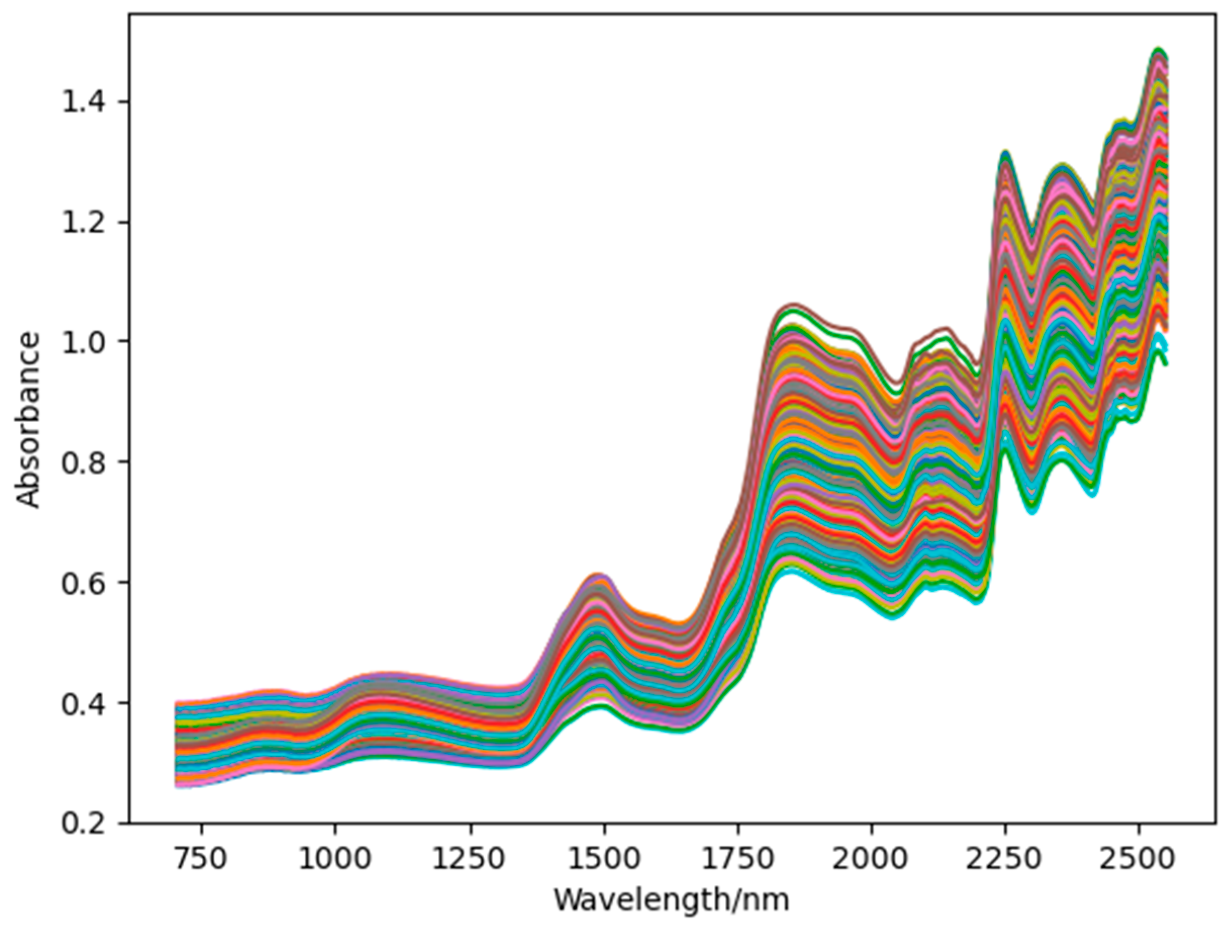
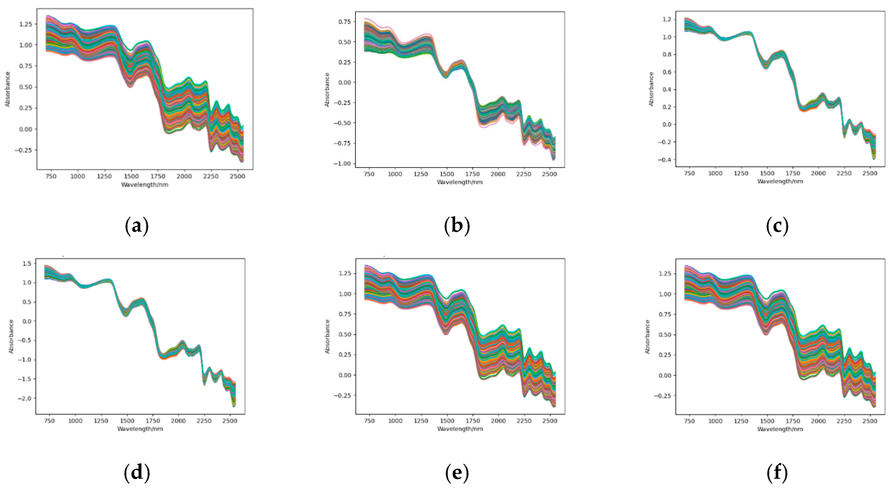
3.1. Spectral Acquisition and Preprocessing

The NIR spectra of maize seeds originating from various sources are illustrated in Figure 4.

The spectral curve graph in Figure 5 illustrates the optimization effect of various pretreatment methods on the original spectral curve of maize seeds. Initially, FD was employed to correct the baseline drift of the original spectral curve of maize seeds, as depicted in Figure 5a. Subsequently, five other preprocessing techniques were applied to mitigate noise in the raw spectra of maize seeds. Among them, FDCT, FDMA, and FDSG processing exhibited negligible impacts (Figure 5b,e,f), while FDMSC and FDSNV demonstrated superior noise elimination efficacy (Figure 5c,d).

The results of different preprocessing techniques under the PLSR model are presented in Figure 6, where a reference line is included to facilitate the observation of linear changes in the data. When the two points progressively approach this auxiliary line it indicates a stable model effect. The blue dots in the figure depict the actual values, whereas the red dots illustrate the model predictions. In Figure 6a, the original spectra exhibit linear changes; however, they appear excessively concentrated and display an evident offset relationship with the reference line. Similar situations occur in Figure 6b–f, after applying FD, FDMSC, FDMA, FDSG, and FDCT processing, respectively. Predicted values demonstrate linear changes with actual values; nevertheless, these preprocessing methods result in uniformly distributed offsets from the reference line leading to high overall prediction errors. In Figure 6c,d, when only MSC and SNV processing without FD preprocessing are applied, there is a centrally heterogeneous distribution of predicted and actual values with noticeable boundaries resulting in faceted changes throughout. In Figure 6e, after FDSNV processing is performed on both predicted and actual values, a linear trend is observed with minimal differences between them; moreover, most of these values align directly on the auxiliary line. Therefore, the NIRS data after FDSNV processing yield optimal results.

The PLSR model was established based on Equations (1)–(4). The correlation coefficient R, the coefficient of determination R², the corrected root mean squared error RMSE, and the standard error SE were calculated for both the calibration set and the prediction set (refer to

Table 2. Analysis of results of different pretreatment methods.

Method	Correction Set				Prediction Set
	R2c	RMSEC	SEC	Rc	R2p	RMSEP	SEP	Rp
RAW	0.974	0.004	0.008	0.987	0.974	0.004	0.008	0.987
FD	0.989	0.008	0.012	0.995	0.989	0.008	0.012	0.995
MSC	0.989	0.002	0.004	0.994	0.988	0.002	0.004	0.994
SNV	0.989	0.007	0.012	0.994	0.989	0.007	0.012	0.994
FDSNV	0.996	0.005	0.002	0.998	0.996	0.005	0.002	0.998
FDMSC	0.985	0.005	0.017	0.993	0.985	0.005	0.017	0.993
FDMA	0.989	0.008	0.012	0.995	0.989	0.008	0.012	0.995
FDSG	0.989	0.008	0.013	0.994	0.989	0.008	0.013	0.994
FDCT	0.988	0.011	0.015	0.994	0.988	0.011	0.015	0.994

). As presented in Table 2, the PLSR model was constructed using raw spectral data. The values are 0.974 for R²_c and R²_p, 0.004 for RMSEC and RMSEP, 0.008 for SEC and SEP, and 0.987 for R_c and R_p. The smaller R²_c/R²_p values observed in comparison to the PLSR models constructed using the FDCT, FDMSC, FDMA, FDSG, and FDSNV algorithms suggest the presence of potential noise or background interference in the raw spectral data, leading to diminished model performance with a larger margin of error. Furthermore, the PLSR model established using MSC/SNV algorithms displayed improved performance/stability due to their capability to effectively eliminate uneven distribution effects caused by sample particles or variations in light range. The FDSNV algorithm, out of the five established PLSR models, exhibits the highest R²_p value of 0.996, surpassing the RAW, FDMSC, FDMA, FDSG, and FDCT algorithms by improvements of 0.022, 0.011, 0.007, and 0.008, respectively. The R_p value of 0.998 indicates a significant improvement compared to the RAW, FDMSC, FDMA, FDSG, and FDCT algorithms with enhancements of 0.011, 0.005, 0.003, 0.004, and 0.004, respectively. The RMSEP value is 0.005, which exhibits reductions of −0.001, 0, 0.003, 0.0033, and 0.006 in comparison to the RAW, FDMSC, FDMA, FDSG, and FDCT algorithms, respectively. Moreover, the SEP value of 0.002 demonstrates a decrease of 0.006 and 0.015 when compared to the RAW and FDMSC algorithms, respectively; it also showcases reductions of 0.010, 0.011, and 0.013 in relation to the FDMA, FDSG and FDCT algorithms, correspondingly. This indicates that the utilization of the FDSNV algorithm for data processing in establishing the PLSR model has resulted in achieving superior accuracy and stability. The results demonstrated that the model established after implementing the FDSNV algorithm exhibited superior performance. This can be attributed to the algorithm’s ability to enhance information visibility in both peak and valley regions of the original spectral data curve of maize seeds, thereby improving the signal-to-noise ratio and highlighting crucial information for the subsequent extraction of characteristic wave numbers. Consequently, the FDSNV algorithm was identified as the preferred preprocessing method for near-infrared spectral data in studies pertaining to maize seed origin identification.

3.2. Building Datasets

To accommodate the convolutional neural network architecture and improve prediction accuracy, the converted spectrograms were rotated for enhancement, as illustrated in Figure 7, due to variations in sample size across different origins. The enhanced spectrograms were then partitioned into training and test sets at a ratio of 3:1. Specifically, each origin had a training set comprising 240 images and a test set containing 80 images. Further details on dataset division are presented in

Table 3. Taxonomic information of origin.

Labels	Original Code	Train	Test
Gansu Suke Sweet 1506	A1	120	40
Gansu huanai color sweet glutinous 102	L	120	40
Shandong Suke Sweet 1506	A2	60	20
Shandong Star Sweet 230	C1	60	20
Shandong Moxidome	D1	60	20
Shandong Golden Sweet 13	H	60	20
Beijing Star Sweet 230	C2	80	26
Beijing Honey Blossom Sweet Glutinous 3	F	80	27
Beijing Star Sweet 221	G	80	27
Shanxi Golden Queen	J	80	26
Shanxi Black Sticky 301	K	80	27
Shanxi Huagnuo 2	B1	80	27
Hebei Zhongnong Sweet 488	I	120	40
Hebei Huagnuo 2	B2	120	40
Jiangsu Ink Pupil	D2	240	80
Xinjiang Tiangui Glutinous 932	E1	240	80
Guangxi Tiangui Glutinous 932	E2	240	80

.

3.3. Effect of Batch Size on Modeling

To enhance convergence performance, gradient stability, generalization, and meet the memory requirements of the model, a small batch size can induce unstable gradients during computation, resulting in significant training oscillation and hindered convergence [28]. Conversely, an excessively large batch size may lead to local optima and subpar generalization performance. Therefore, a batch size test is devised to determine the optimal value.

The results of experiments with different batch sizes are presented in

Table 4. Prediction results of different batch sizes.

Batch_Size	Train/%	Test/%	Time/mins
16	90.59	69.85	54.26
32	96.93	89.06	57.15
48	98.7	93.75	56.35
64	97.55	71.41	66.83
128	96.81	81.63	72.98

. When the batch size is set to 48, the training set accuracy reaches 98.7%, which demonstrates an improvement of 8.11%, 1.77%, 1.15%, and 1.89% compared to batch sizes of 16, 32, 64, and 128, respectively. Notably, a batch size of 48 exhibits the most significant effect on performance enhancement. Furthermore, altering the batch sizes from 16, 32, 64, and 128 leads to improvements in test set accuracy by percentages of 20.9%, 4.69%, 22.34%, and 12.12%, respectively. The test set accuracy ultimately achieves 93.75%. In terms of training time, using a batch size of 48 requires only an additional 2.09 min compared to a batch size of 16. It reduces training time by 0.8 min when compared to a batch size of 32 and even more significantly by 66.83 min and 16.63 min when compared to batches of 64 and 128, respectively. Therefore, setting the optimal batch size as 48 is highly suitable as it enhances memory utilization, speeds up processing speed, reduces training time, stabilizes model performance, enhances generalization performance, makes gradient direction more accurate, reduces training oscillations, and achieves better convergence.

3.4. Impact of Learning Rate on the Model

The learning rate experiment is designed to analyze and compare the effects of different learning rates on the model [29], with a batch size of 48 and 300 training rounds, in order to determine the optimal learning rate. Setting an excessively high learning rate will impede network convergence, while setting it too low will result in sluggish convergence and a prolonged search for the optimal value. The results of various learning rate experiments are presented in

Table 5. Prediction results of different learning rates.

Learning Rate	Train/%	Test/%	Time/mins
10−3	51.04	42.03	55.7
10−4	83.33	79.53	58.52
10−5	97.11	92.66	53.57
10−6	95.74	93.91	53.99
10−7	100	97.03	54.18
5−7	100	95.94	57.7
10−8	100	92.97	53.7
10−9	64.69	62.97	59.8

.

The analysis results indicate that the training time of the model is minimally affected by the learning rate. Optimal prediction results are achieved at learning rates of 10⁻⁷, 5⁻⁷, and 10⁻⁸, respectively. However, careful examination of the accuracy curve reveals inadequate convergence when using learning rates of 10⁻⁷ and 5⁻⁷. Overfitting occurs with a learning rate of 10⁻⁹. Hence, it can be concluded that a learning rate of 10⁻⁸ is optimal.

3.5. Impact of Dropout on the Model

The network structure is optimized using the Dropout method to mitigate overfitting. By disregarding fixed weight features in each training batch [30], Dropout effectively reduces feature correlation, thereby enhancing the model’s global nature, improving generalization capability, and preventing overfitting.

The results of various Dropout experiments are presented in

Table 6. Prediction results of different Dropout values.

Dropout	Train/%	Test/%
0.3	100	92.97
0.4	100	94.38
0.5	100	95.61
0.6	100	95.31
0.7	100	94.69

, and the comparative findings suggest that configuring the Dropout to 0.5 significantly enhances model performance. In comparison to Dropout settings of 0.3, 0.4, 0.6, and 0.7, there is an observed improvement in prediction set accuracy by 2.64%, 1.23%, 0.3%, and 0.92%, respectively, thereby confirming the optimal value for Dropout as indeed being 0.5.

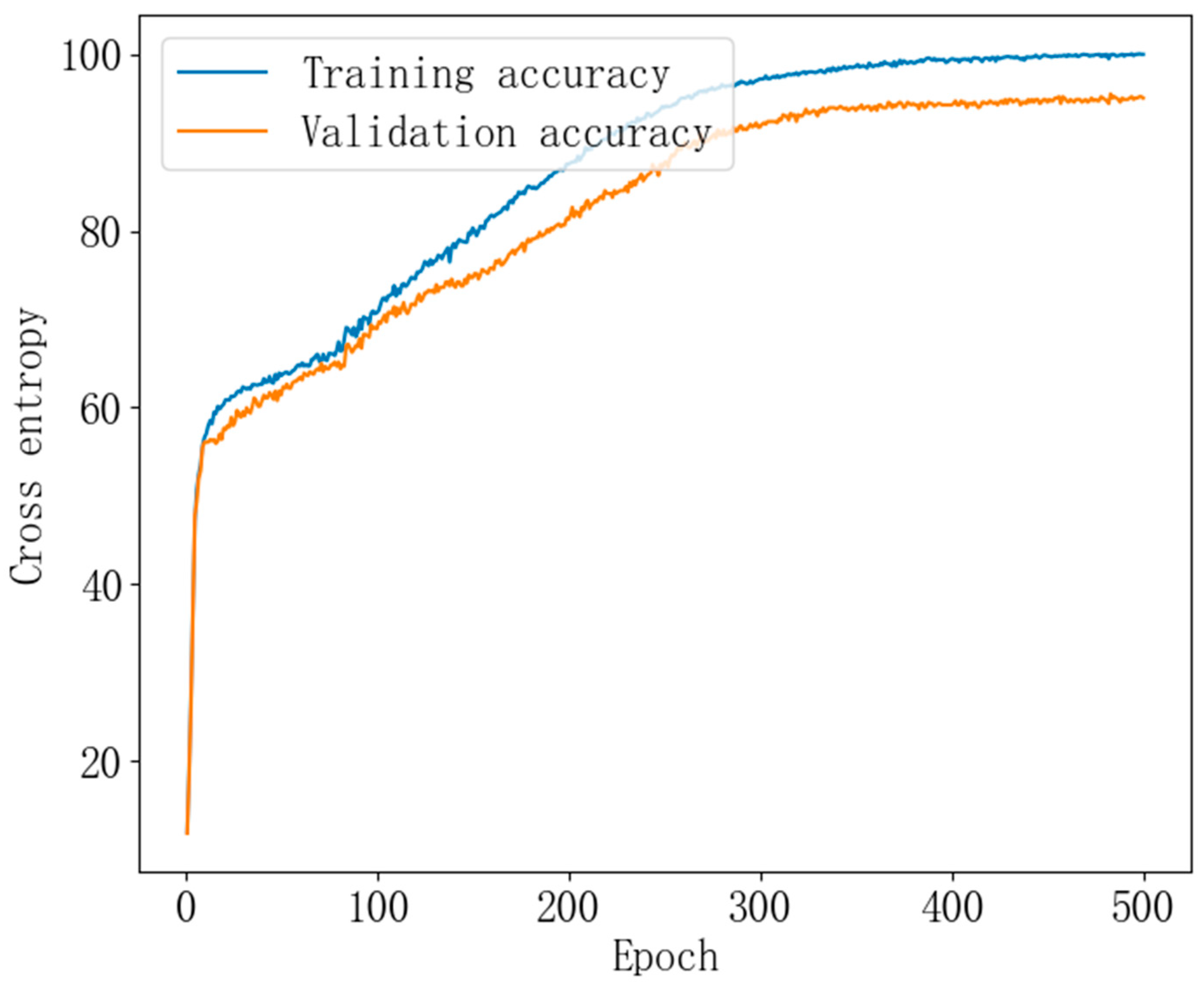
3.6. Maize Seed Origin Identification Model Prediction Results

The batch size is set to 48, the learning rate is set to 10⁻⁸, Dropout is set to 0.5, and the number of training iterations for network training is determined as 500 based on parameter adjustment results. The model’s training accuracy can be observed in Figure 8, while the loss function is illustrated in Figure 9. As the number of network iterations increases to 340 rounds, the model demonstrates a tendency towards stability and convergence.

The predictions of the model are depicted in Figure 10. The top row illustrates the actual origin, while the bottom row represents the predicted origin.

3.7. Model Comparison

The study conducted by Silva et al. [31] utilized PCA for the analysis of fourteen compounds found in guarana seeds, enabling differentiation between seeds from Bahia and Amazonas. In order to validate the model, PCA was employed to determine the origin of maize seeds, as illustrated in Figure 11. As depicted in Figure 11a, PC1 and PC2 account for 76.88% and 17.23%, respectively, resulting in a cumulative contribution of 94.11%. These two principal components sufficiently explain most of the variables under consideration. From Figure 11b, it can be observed that there is no discernible clustering among different origins of maize seeds; instead, they exhibit a dispersed and intersecting pattern.

The analysis results of the models constructed using each method are presented in

Table 7. Comparison of test results.

Method	Accuracy	Recall/ Sensitivity	Specificity	Precision
RAW	40.08	88.65	34.53	37.35
PCA	40.65	90.47	36.28	39.28
GAF-VGG	96.81	97.23	95.35	95.12

. In terms of accuracy, recall, specificity, and precision (96.81%, 97.23%, 95.35%, and 95.12%), the GAF-VGG network model exhibits significant superiority over both the original data and the PCA-based origin identification model. This can be attributed to the fact that PCA, being an unsupervised learning technique, fails to effectively capture discriminative features due to minimal variations in spectral information among different origins. Moreover, downsizing with PCA may lead to the loss of valuable information and features owing to the complexity and redundancy of NIR spectral data. Conversely, as a supervised learning approach, the GAF-VGG model accurately selects origin-specific features for maize seeds, thereby enhancing their identification accuracy and enabling high-precision analysis. However, distinguishing between origins becomes challenging due to similar compounds such as protein, fat, and starch present in maize seeds which result in near-infrared spectral curves exhibiting comparable characteristic peaks; hence, achieving a prediction accuracy of 100% is arduous.

4. Conclusions

A rapid and non-destructive identification model for maize seeds of different origins was developed using near-infrared spectroscopy combined with chemometrics. The spectral data of maize seeds from various sources were acquired while ensuring sample integrity. The spectra were optimized using first-order derivatives in conjunction with SNV, and the one-dimensional spectral features were extracted and transformed into three-dimensional images using GAF. Origin identification models for maize seeds were established utilizing PCA and VGG networks, respectively. The results demonstrated the following:

(1)

GAF leverages the correlation between the one-dimensional NIR spectrum and the time series to enhance the informative content, effectively extracting data from the one-dimensional NIR spectrum. The GAF method solely requires converting the NIR spectrum into an image without involving feature extraction, enabling a more intuitive analysis of NIR spectral data and efficiently addressing the issue of laborious characteristic wavelength extraction. By integrating this converted three-dimensional image with VGG, extensively utilized for large-scale image analysis, we can further discern distinctive features of maize seeds originating from diverse sources. Only adjustments to inputs and specific parameters of the VGG network are necessary to achieve superior results compared to traditional methods, thereby simplifying complexity in NIR spectral modeling.

(2)

The combination of preprocessing and PCA cannot achieve high-precision identification analysis of maize seeds from different origins. However, the GAF-VGG network can perform feature extraction under complex conditions with both high and stable prediction accuracy. This network is capable of identifying maize seeds that do not possess the characteristics of their respective origins, providing a new perspective for origin identification and traceability analysis in maize seeds. The results achieved using the GAF-VGG network model outperformed those of Schütz et al. [32], who accurately predicted the origin of maize seeds with 95% accuracy using Fourier Transform NIR spectroscopy and SVM methods, thus emphasizing the advantages of integrating GAF with VGG network for identifying maize seed origins.

(3)

The quality and characteristics of a seed can be influenced by its origin. By promptly identifying the origin of maize seeds, growers are able to exercise better control over seed quality, select seeds that are suitable for local climate and soil conditions, enhance crop adaptability and resistance, as well as reduce the occurrence of pests and diseases. Ultimately, this leads to improved crop yield and quality. Certain regions may have specific pests or diseases prevalent in their agricultural systems. Identifying the origin of a seed enables tracing back to its source location, facilitating timely detection and monitoring of pest and disease spread. This aids in implementing appropriate control measures to ensure healthy crop growth. In the marketplace, information regarding the origin of maize seeds is crucial for both consumers and traders alike. Swift identification of seed origins ensures market credibility by enhancing product quality standards and safety while also boosting market competitiveness. To summarize, rapid identification of maize seed origins significantly contributes to quality control measures, epidemic monitoring efforts, market traceability initiatives, as well as improving production efficiency levels while ensuring stable agricultural development.

(4)

Future work should focus on further improving identification techniques and methods, such as enhancing spectrogram conversion and exploring the combination of different spectral preprocessing techniques and conversion methods to reduce the number of features in the generated spectral images that do not meet the requirements. Additionally, efforts should be made to enhance the accuracy and speed of identification, reduce costs, and improve anti-interference capabilities. This may involve innovations in sensor technology, image processing algorithms, machine learning models, etc. Furthermore, it is important to develop portable identification devices that can be easily used in the field to provide growers with instant information about seed origin. This will offer growers more flexibility and convenience in seed selection and management. Moreover, it is necessary to apply seed origin identification technology to seed quality testing and origin traceability for other crops like wheat and soybean in order to cater to the needs of growers from various agricultural sectors. Establishing a data-sharing platform for seed origin identification is crucial for promoting the exchange and sharing of seed information. Simultaneously, promoting formulation and unification of relevant standards is important for improving the standardization level and universality of seed origin identification technology. In summary, future advancements in rapid maize seed origin identification will focus on technological improvements, the development of portable equipment, application expansion, and data sharing to provide more reliable and efficient services for seed quality management and origin tracing in agricultural production.

References

1. Shakiba, N.; Gerdes, A.; Holz, N.; Wenck, S.; Bachmann, R.; Schneider, T.; Seifert, S.; Fischer, M.; Hackl, T. Determination of the geographical origin of hazelnuts (Corylus avellana L.) by Near-Infrared spectroscopy (NIR) and a Low-Level Fusion with nuclear magnetic resonance (NMR). Microchem. J. 2022, 174, 107066. [Google Scholar] [CrossRef]
2. Varrà, M.O.; Ghidini, S.; Ianieri, A.; Zanardi, E. Near infrared spectral fingerprinting: A tool against origin-related fraud in the sector of processed anchovies. Food Control 2021, 123, 107778. [Google Scholar] [CrossRef]
3. Leiva, S.F.; Sandoval, J.L.; Abascal-Ponciano, G.A.; Flees, J.J.; Calderon, A.J.; Pacheco, W.J.; Starkey, C.W. Improper sample preparation negatively affects near infrared reflectance spectroscopy (NIRS) nutrient analysis of ground corn. Anim. Feed. Sci. Technol. 2022, 293, 115472. [Google Scholar] [CrossRef]
4. Song, C.; Peng, B.; Wang, H.; Zhou, Y.; Sun, L.; Suo, X.; Fan, X. Maize seed appearance quality assessment based on improved Inception-ResNet. Front. Plant Sci. 2023, 14, 1249989. [Google Scholar] [CrossRef] [PubMed]
5. He, X.; Liu, L.; Liu, C.; Li, W.; Sun, J.; Li, H.; He, Y.; Yang, L.; Zhang, D.; Cui, T.; et al. Discriminant analysis of maize haploid seeds using near-infrared hyperspectral imaging integrated with multivariate methods. Biosyst. Eng. 2022, 222, 142–155. [Google Scholar] [CrossRef]
6. Febrianto, N.A.; Zhu, F. Composition of methylxanthines, polyphenols, key odorant volatiles and minerals in 22 cocoa beans obtained from different geographic origins. LWT 2022, 153, 112395. [Google Scholar] [CrossRef]
7. Wei, X.; Zhou, Y.; Jiang, Y.; Tsang, D.C.; Zhang, C.; Liu, J.; Zhou, Y.; Yin, M.; Wang, J.; Shen, N.; et al. Health risks of metal (loid) s in maize (Zea mays L.) in an artisanal zinc smelting zone and source fingerprinting by lead isotope. Sci. Total Environ. 2020, 742, 140321. [Google Scholar] [CrossRef]
8. Moghaddam, H.N.; Tamiji, Z.; Lakeh, M.A.; Khoshayand, M.R.; Mahmoodi, M.H. Multivariate analysis of food fraud: A review of NIR based instruments in tandem with chemometrics. J. Food Compos. Anal. 2022, 107, 104343. [Google Scholar] [CrossRef]
9. Mansuri, S.M.; Chakraborty, S.K.; Mahanti, N.K.; Pandiselvam, R. Effect of germ orientation during Vis-NIR hyperspectral imaging for the detection of fungal contamination in maize kernel using PLS-DA, ANN and 1D-CNN modelling. Food Control 2022, 139, 109077. [Google Scholar] [CrossRef]
10. Arena, E.; Campisi, S.; Fallico, B.; Maccarone, E. Distribution of fatty acids and phytosterols as a criterion to discriminate geographic origin of pistachio seeds. Food Chem. 2007, 104, 403–408. [Google Scholar] [CrossRef]
11. de Oliveira Salles, R.C.; Muniz, M.P.; Nunomura, R.D.C.S.; Nunomura, S.M. Geographical origin of guarana seeds from untargeted UHPLC-MS and chemometrics analysis. Food Chem. 2022, 371, 131068. [Google Scholar] [CrossRef]
12. Zheng, Y.; Cao, Y.; Yang, J.; Xie, L. Enhancing model robustness through different optimization methods and 1-D CNN to eliminate the variations in size and detection position for apple SSC determination. Postharvest Biol. Technol. 2023, 205, 112513. [Google Scholar] [CrossRef]
13. Vitale, R.; Bevilacqua, M.; Bucci, R.; Magrì, A.D.; Magrì, A.L.; Marini, F. A rapid and non-invasive method for authenticating the origin of pistachio samples by NIR spectroscopy and chemometrics. Chemom. Intell. Lab. Syst. 2013, 121, 90–99. [Google Scholar] [CrossRef]
14. Jin, X.; Zhou, J.; Rao, Y.; Zhang, X.; Zhang, W.; Ba, W.; Zhou, X.; Zhang, T. An innovative approach for integrating two-dimensional conversion of Vis-NIR spectra with the Swin Transformer model to leverage deep learning for predicting soil properties. Geoderma 2023, 436, 116555. [Google Scholar] [CrossRef]
15. Li, Y.; Chen, Z.; Zhang, F.; Wei, Z.; Huang, Y.; Chen, C.; Zheng, Y.; Wei, Q.; Sun, H.; Chen, F. Research on detection of potato varieties based on spectral imaging analytical algorithm. Spectrochim. Acta Part A Mol. Biomol. Spectrosc. 2024, 311, 123966. [Google Scholar] [CrossRef]
16. Tan, A.; Wang, B.; Zhao, Y.; Wang, Y.; Zhao, J.; Wang, A.X. Near-infrared spectroscopy analysis of compound fertilizer based on GAF and quaternion convolution neural network. Chemom. Intell. Lab. Syst. 2023, 240, 104900. [Google Scholar] [CrossRef]
17. Carvalho, J.K.; Moura-Bueno, J.M.; Ramon, R.; Almeida, T.F.; Naibo, G.; Martins, A.P.; Santos, L.S.; Gianello, C.; Tiecher, T. Combining different pre-processing and multivariate methods for prediction of soil organic matter by near infrared spectroscopy (NIRS) in Southern Brazil. Geoderma Regional. 2022, 29, e00530. [Google Scholar] [CrossRef]
18. An, M.; Cao, C.; Wang, S.; Zhang, X.; Ding, W. Non-destructive identification of moldy walnut based on NIR. J. Food Compos. Anal. 2023, 121, 105407. [Google Scholar] [CrossRef]
19. Bian, X.; Wang, K.; Tan, E.; Diwu, P.; Zhang, F.; Guo, Y. A selective ensemble preprocessing strategy for near-infrared spectral quantitative analysis of complex samples. Chemom. Intell. Lab. Syst. 2020, 197, 103916. [Google Scholar] [CrossRef]
20. Arianti, N.D.; Saputra, E.; Sitorus, A. An automatic generation of pre-processing strategy combined with machine learning multivariate analysis for NIR spectral data. J. Agric. Food Res. 2023, 13, 100625. [Google Scholar] [CrossRef]
21. Wang, M.; Xu, Y.; Yang, Y.; Mu, B.; Nikitina, M.A.; Xiao, X. Vis/NIR optical biosensors applications for fruit monitoring. Biosens. Bioelectron. X 2022, 11, 100197. [Google Scholar] [CrossRef]
22. de Almeida, A.G.; Tormena, C.D.; de Aguiar, N.S.; Wendling, I.; Rakocevic, M.; Pauli, E.D.; Scarminio, I.S.; Bruns, R.E.; Marcheafave, G.G. Direct NIR spectral determination of genetic improvement, light availability, and their interaction effects on chemically selected yerba-mate leaves. Microchem. J. 2023, 191, 108828. [Google Scholar] [CrossRef]
23. Chen, R.; Li, S.; Cao, H.; Xu, T.; Bai, Y.; Li, Z.; Leng, X.; Huang, Y. Rapid quality evaluation and geographical origin recognition of ginger powder by portable NIRS in tandem with chemometrics. Food Chem. 2024, 438, 137931. [Google Scholar] [CrossRef]
24. Schoot, M.; Kapper, C.; van Kollenburg, G.H.; Postma, G.J.; van Kessel, G.; Buydens, L.M.; Jansen, J.J. Investigating the need for preprocessing of near-infrared spectroscopic data as a function of sample size. Chemom. Intell. Lab. Syst. 2020, 204, 104105. [Google Scholar] [CrossRef]
25. Lee, H.; Yang, K.; Kim, N.; Ahn, C.R. Detecting excessive load-carrying tasks using a deep learning network with a Gramian Angular Field. Autom. Constr. 2020, 120, 103390. [Google Scholar] [CrossRef]
26. Qi, P.; Chiaro, D.; Piccialli, F. FL-FD: Federated learning-based fall detection with multimodal data fusion. Inf. Fusion 2023, 99, 101890. [Google Scholar] [CrossRef]
27. Lu, Y.; Wu, X.; Liu, P.; Li, H.; Liu, W. Rice disease identification method based on improved CNN-BiGRU. Artif. Intell. Agric. 2023, 9, 100–109. [Google Scholar] [CrossRef]
28. Min, W.; Wang, Z.; Yang, J.; Liu, C.; Jiang, S. Vision-based fruit recognition via multi-scale attention CNN. Comput. Electron. Agric. 2023, 210, 107911. [Google Scholar] [CrossRef]
29. Li, J.; Zhu, Z.; Liu, H.; Su, Y.; Deng, L. Strawberry R-CNN: Recognition and counting model of strawberry based on improved faster R-CNN. Ecol. Inform. 2023, 77, 102210. [Google Scholar] [CrossRef]
30. Aishwarya, M.P.; Reddy, P. Ensemble of CNN models for classification of groundnut plant leaf disease detection. Smart Agric. Technol. 2023, 6, 100362. [Google Scholar]
31. da Silva, G.S.; Canuto, K.M.; Ribeiro, P.R.V.; de Brito, E.S.; Nascimento, M.M.; Zocolo, G.J.; Coutinho, J.P.; de Jesus, R.M. Chemical profiling of guarana seeds (Paullinia cupana) from different geographical origins using UPLC-QTOF-MS combined with chemometrics. Food Res. Int. 2017, 102, 700–709. [Google Scholar] [CrossRef] [PubMed]
32. Schütz, D.; Riedl, J.; Achten, E.; Fischer, M. Fourier-transform near-infrared spectroscopy as a fast screening tool for the verification of the geographical origin of grain maize (Zea mays L.). Food Control 2022, 136, 108892. [Google Scholar] [CrossRef]
Figure 1. Sample of maize. The figure illustrates maize seeds of various origins, denoted by (AL), which were utilized in the experiment. The numbers in the figure correspond to the origin codes in Table 1.
Agriculture 14 00466 g001
Figure 2. Dataset production process. The entire process involves segmenting the raw spectral data for approximate aggregation, transferring it to the polar coordinate system, and ultimately generating GASF and GADF maps. The yellow arrows serve as a guiding indicator for advancing to the next step; GADF and GASF color maps depict the spectrograms that have been transformed. The colors in the figure, such as blue, are associated with the pixel values that each value maps to [0–255].
Agriculture 14 00466 g002
Figure 3. Improved VGGNet model. The data structure from the input layer to the conv5 layer has a width and height of 32. The structure for conv1 is 32 × 32 × 64, for conv2 is 32 × 32 × 128, for conv3 is 32 × 32 × 256, for conv4 is 32 × 32 × 512, and for conv5 it remains as 32 × 32 × 512.
Agriculture 14 00466 g003
Figure 4. Spectral curve of maize seeds. Each line represents a spectral curve.
Agriculture 14 00466 g004
Figure 5. Spectral curve after preprocessing: (a) FD preprocessing; (b) FDCT preprocessing; (c) FDMSC preprocessing; (d) FDSNV preprocessing; (e) FDMA preprocessing; (f) FDSG preprocessing. The CSV data file allows for direct subsequent grouping to be performed.
Agriculture 14 00466 g005
Figure 6. Results of different preprocessing under PLSR model: (a) PLSR model predictions for RAW; (b) PLSR model predictions for FD; (c) PLSR model predictions for MSC; (d) PLSR model predic–tions for SNV; (e) PLSR model predictions for FDSNV; (f) PLSR model predictions for FDMSC; (g) PLSR model predictions for FDMA; (h) PLSR model predictions for FDSG; (i) PLSR model predictions for FDCT. The closer the data points on the graph are to the regression line, the higher the level of processing efficiency will be.
Agriculture 14 00466 g006aAgriculture 14 00466 g006b
Figure 7. Three ways to perform data enhancement of spectral images: (a) original image; (b) original image rotated 90 degrees to the left; (c) rotate the original image 180 degrees; (d) rotate the original image 90 degrees to the right.
Agriculture 14 00466 g007
Figure 8. Model training accuracy.
Agriculture 14 00466 g008
Figure 9. Model training loss function.
Agriculture 14 00466 g009
Figure 10. Prediction results of the GAF-VGGNet model. The values depicted in the figure represent feature points, where both the horizontal and vertical coordinates consist of 32 feature points that correspond to the converted spectrogram.
Agriculture 14 00466 g010
Figure 11. Predictions from the PCA model: (a) contribution vs. cumulative contribution plots for the PCA model, with component contributions shown in red and cumulative contributions shown in blue; (b) the PCA method yields results for predicting origins. The color of each origin corresponds to the figure legend in the upper right corner.
Agriculture 14 00466 g011