Abstract
Alfalfa (Medicago sativa L.) is used to support livestock. A stability study was carried out over three years. The stability indices for yield and main quality characteristics such as plant height, number of nodes, the yield of green mass and dry matter, crude protein and fiber (%), and ash (%), were examined. Statistical analysis revealed significant differences that indicated the presence of high genotype–year interactions. Heritability was higher in the case of qualitative traits than quantitative traits. The most intriguing correlation was between green mass yield and crude protein content because positive correlations may lead to indirect and simultaneous selection. According to the statistical biplot models AMMI and GGE, the best genotypes for almost all traits to use, regardless of the environment and cultivation type, were the G8 (Population 2) followed by cultivar G3 (Yliki). Despite the high index values shown by the parameter number of nodes, the latter and yield showed low heritability.
1. Introduction
The crop alfalfa (Medicago sativa L.) supports livestock in many places in the world; thus, its yield and quality are of great importance to the farmers who use it as an animal feed [1,2]. In addition, it adds nitrogen to the soil, improving the productivity of following crops, while its biomass contributes to the productivity of animals [3]. The genetic and phenotypic variability in alfalfa cultivars [4] allows its cultivation in various environments. The cultivars and populations of alfalfa that have been developed after an intense selection resulted in resistance to diseases, drought, or cold [5]. Undeniably, alfalfa represents a significant crop for farming in many places of the world [6]. Alfalfa is rich in protein, diverse nutrients, minerals, and numerous vitamins [6,7]. Other reports state that dry matter contains organic materials, fibers, proteins and fats, and anti-inflammatory and immunostimulatory agents, much more than other grass species [8,9].
Fahad et al. [10], Kebede et al. [11], Odeseye et al. [12], Wayu and Atsbha [13], and Atumo et al. [3] reported different behavior in yields across years and areas of cultivation, and in other words, different response to environments. Alfalfa exhibits broad adaptation capability in different environments [14]. A breeder has to propose alfalfa varieties suitable for different environments, whereas farmers must introduce this valuable crop into cultivation in order to support livestock [6,15]. Selection in a breeding program is based mainly on yield stability and high quality [16]. Experimental populations are the first step in breeding programs aiming at designing new varieties of a rich gene pool [17,18,19]. Seiam and El-Nahrawy [20] performed modified mass selection to select profitable genotypes in alfalfa. They managed to improve yield and many qualitative characteristics and reported that protein content is of primary concern since it contributes to the quality of animal feed. Their results showed sufficient genotypic variation among selected families useful for their breeding program. Unal et al. [21] reported successful mass selection concerning green forage and dry matter yields during the breeding procedure of alfalfa genetic materials. Furthermore, they concluded that some promising genetic materials may exhibit high and stable yield performance, with good quality. Also, Acharya et al. [22] reported a high and stable improvement of dry matter yield in alfalfa genetic materials that may be utilized in order to develop high performing and well-adopted alfalfa cultivars. Eren et al. [23] analyzed alfalfa genetic diversity and local population structure by molecular markers. They concluded that the iPBS molecular markers can be a helpful tool in identifying parents with high genetic diversity in alfalfa breeding.
As it is known, yield is strongly affected by factors such as genotype (G), environment (E), and genotype x environment interaction (GEI) [24,25,26,27], but, among them, GEI leads genotypes to respond differently in different environments [28]. The literature reports that the cultivation year significantly influences green mass and dry matter yield, as well as the protein content (%) in some species [29]. Differences in the genotype adaptability in various environmental conditions result in problems concerning the choice of cultivar [30]. It was observed that due to the GEI, some premium cultivars of alfalfa are dependent on the environment [31]. As a solution for the GEI, Ceccarelli [32] proposed cultivars of specific adaptation for use in certain environments.
The literature reports different statistical techniques to analyze and explain GEI [33,34]. Two statistical analysis methods, the additive main effect and multiplicative interaction (AMMI) [35] and the genotype-by-environment (GGE) biplot [36], are mostly utilized since they can provide easy to read graphical tools that can give valuable insights about GEI. Especially, the GGE biplot allows the analysis of the genotype for two parameters at the same time (i.e., stability and yielding ability) and, thus, is considered a powerful tool for efficiently examining the multi-environment data in breeding [37].
This study aims to assess three-year environmental conditions and genotypes, to determine how year effects affect alfalfa genotypes’ behaviors, and to suggest the best genotypes based on the stability, using the tool of the stability index [38] for alfalfa yield and main quality traits. The genotypes utilized for this study were six Greek cultivars and four populations derived from Greek ecotypes in western Macedonia by the application of the mass selection method.
2. Materials and Methods
2.1. Plant Material, Environment, and Experimental Design
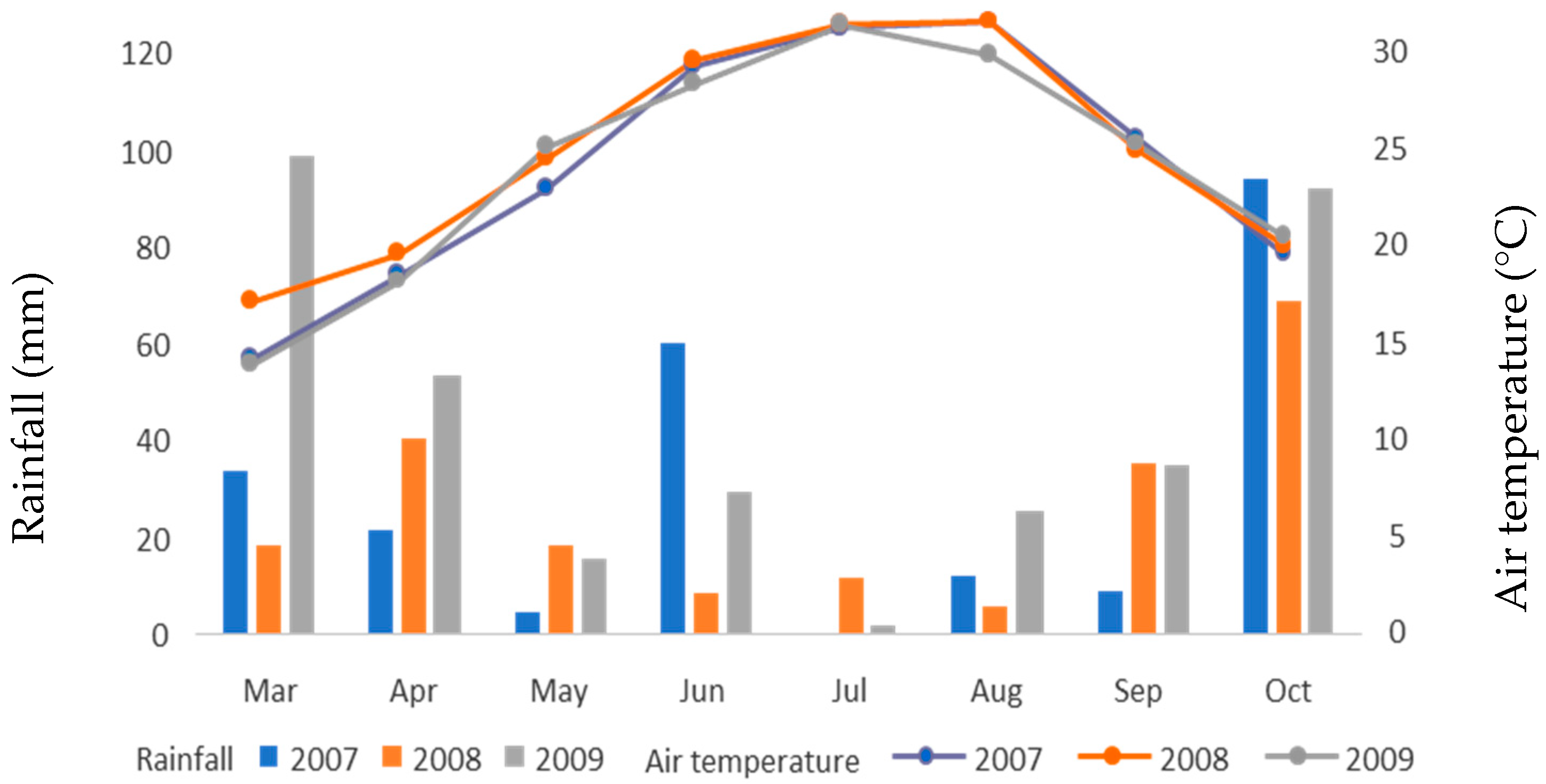
All the experiments were conducted in Trikala, central Greece, for three years, which we consider to be different environmental conditions. Figure 1 shows meteorological data for the three years of experimentation, including mean air temperature (°C) and total monthly rainfall (mm). The sowing was completed within one day on 18 March 2007.
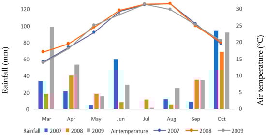
Figure 1.
Meteorological data for the alfalfa period of cultivation (2007–2009).
Six alfalfa varieties, namely G1: Florina, G2: Dolichi, G3: Yliki, G4: Ypati 84, G5: Chaironia, and G6: Chloi, as well as four alfalfa experimental populations—G7: Population 1, G8: Population 2, G9: Population 3, and G10: Population 4—created by Stylianos Zotis were the genetic materials used in the present study. Five varieties (G1 to G5) were obtained from the Institute of Industrial and Forage Crops (Hellenic Agricultural Organization Demeter, Greece). Chloi (G6) was developed by Zouliamis Nikolaos (Servia, Kozani, Greece). Ypati 84 is the first place in the preferences of Greek producers, with high yield and adaptability in various climate. Chloi and Yliki varieties are mid-early, long-lived, and productive with excellent establishment capacity and adaptability in all regions of Greece. Dolihi and Haironia varieties are long-lived, with excellent establishment capacity and are recommended for the warmer regions of the country where they re-grow even in the winter, while Florina is resilient to cold and dry conditions. The G7 to G10 populations were created by applying the mass selection method to Greek ecotypes of the region of western Macedonia.
The chosen experimental design was a randomized complete block, according to Steel et al. [39], in four replications. Each plot consisted of five rows 8 m long, 0.25 m apart, and plant density was as usual for forage grasses (seeding rate was 18 Kg ha−1). The total experimental plot area was 10 m2.
The cultivation techniques were the usual ones followed by all local farmers. P2O5 (0-46-0) was added as a fertilizer (annually 90 Kg ha−1), incorporated into the soil before sowing in the first year, and surface spread every January for the two following years.
2.2. Experimental Measurements
The experimental measurements were performed randomly on ten main stems (one for each crown) in each plot. The following agronomic characteristics were measured just before the harvest:
- (a)
- Plant height: the measurement in centimeters between the top of the stem and the soil.
- (b)
- The number of nodes, expressed as the total number of main stem nodes.
The harvest of the plots was performed mechanically at the onset of flowering (BBCH 60, Enriquez-Hidalgo et al. [40]). A total of eighteen cuts were made during the first to third year of the plant’s life to evaluate populations and cultivars: five in 2007; seven in 2008; and six in 2009. The whole plot area was cut to a height of 5 cm, and the cut was then weighed to determine the green forage yield.
Subsamples of about 500 g of green biomass were obtained from the center of each plot just before cutting and used to measure dry matter yield after drying (at 105 °C, 48 h). The results were expressed in tons per hectare (t ha−1). The sum of the annual cuts was used to calculate the annual forage yields.
The advised official methods [41] were used to assess the chemical composition of the samples. The samples obtained after every cut of the second season were dried at 70 °C before analysis. The crude protein (%) was determined using the Kjeldahl method using the conversion factor of 6.25 (AOAC, 2005) [42]. Crude fiber (%) was determined according to the AOAC method 978.10, which consists of digestions (under acidic and basic conditions), followed by the gravimetrical determination of the remaining residue (AOAC, 2005) [42]. Ash (%) was determined by the incineration of the sample at 600 °C in a furnace for two hours as recommended by the AOAC 942.05 method [42].
2.3. Data Elaboration
The stability index was calculated using, as follows, [24,25,26,27,38,43,44,45,46,47] , where represents the mean value of each parameter examined for every genetic material utilized in this study and s the respective standard deviation. ANOVA was used to assess the data across environments to reveal significant differences for each measured parameter. The following growth seasons were defined as environments: 2007 was Environment 1 (E1), 2008 was Environment 2 (E2), and 2009 was Environment 3 (E3). The data from all harvests within a year were averaged for the statistical analysis. The data were analyzed using a mixed model and two-way analysis of variance (ANOVA), where genotypes were the fixed variable and environment was the random effect [39]. Correlation between traits was analyzed and measured by the Pearson coefficient as suggested in the literature [39]. A level of significance of less than 0.05 was used in all statistical tests performed. All statistical analyses were performed using the software SPSS 25 (International Business Machines—IBM Corporation, Chicago, IL, USA).
The variance was computed using the mean-squared values of the genotypes, genotype environment, error, and replicates, as recommended in the literature [48]. This allowed the establishment of the genetic parameters for the attributes under study. The heritability in a broad sense (H2) was computed based on literature suggestions [49,50], as follows:
For each evaluated attribute, the phenotypic coefficient of variation (PCV) and genotypic coefficient of variation (GCV) were calculated based on the following equations [51]:
where the genotypic variance, phenotypic variance, genotype × environment variance, residual variance (error), number of replications, number of environments, and overall mean for every examined attribute are, in turn, denoted by , , , , r, e, and , respectively.
2.4. Biplot Models
There are two widely used biplot models:
AMMI biplot = the additive main effects and multiplicative interaction and,
GGE biplot = genotype + genotype × environment.
The analysis of variance of the genotype and environment main effects with the PCA of the GEI generates the AMMI model, while the AMMI or GEI biplot is performed based on the SVD of a double-centered G × E table [52,53].
The AMMI analysis was used to depict the genotype × environment interaction via software using multi-environment data for analysis. The AMMI produces two-way tables, and the estimated least-squares are used to extract a two-way ANOVA for studying the factor’s main effects. In this manner, a value showing the residual interaction is estimated [54]. Besides the adaptation figure map, AMMI can generate a biplot with the factor and Principal Component 1 (PC1) projected on the X and Y axes, respectively. When the PC1 value is low, the genotype is placed near the X axis, suggesting that it is the more stable among all environments.
The concept of the biplot was first developed by Gabriel [55]. It is a scatter plot that graphically displays both the entries (e.g., cultivars) and the testers (e.g., environments) of two-way data (http://www.ggebiplot.com/concept.htm, accessed on 13 February 2024).
In breeding and genetics data, testers can also be traits, genetic markers, etc. GGE analyses simultaneously genotype main effect (G) with genotype by environment interaction (GEI), revealing the main portion of the variance. The GGE matrix includes genotype by environment (G × E) data without environment means. The generated biplot depicts the GGE of a genotype affected by the environment [36,37].
GGE biplots reveal that the most stable and desirable environments are those placed near the average and ideal environment and the genotypes with high desirability are located close to the ideal genotype.
Statistical analysis was performed using the PB tools v.1.4. (free version) software of the International Rice Research Institute (IRRI, Laguna, Philippines).
2.5. Exploratory Data Analysis
Exploratory data analysis was based on cluster analysis and heat tables. Ward’s method was used to process the data mathematically in hierarchical cluster analysis (HCA). JMP 14 (SAS Institute Inc., Cary, NC, USA) was used to conduct the HCA analysis. A dendrogram is used to display the cluster analysis results.
Also, a scaled principal components analysis (PCA) was performed in order to explain the variability and the contribution of the characteristics studied. A two-stage technique was used.
3. Results
3.1. Variation in the Stability Indices
Table 1 reports ANOVA results for the yield and quality traits of alfalfa. Statistically significant differences were observed at the 0.05 level for all the parameters studied, except for all G × Y interactions (GEI) that were significant at the p < 0.01 level.

Table 1.
Mean squares (m.s.) from an ANOVA for the evaluated attributes across years and genotypes.
Table 2 presents stability indices for all traits. Crude fiber (%) showed the highest stability indices. Five genetic materials exceeded 10,000, whereas in the case of Population 3, 50,000 was exceeded, which is a very extreme value. Crude protein content (%) also showed high values for three genetic materials (near or over 10,000 and up to 20,000). The third qualitative trait, ash content, also showed high values (over 6000 in two cases). Plant height is a quantitative trait with high values. Yield showed the lowest values, whereas variety Dolichi and Population 4 showed the highest values for green mass. Ypati 84, Yliki, and Dolichi showed the highest stability values for dry matter yield. Populations 2, 3, and 4 showed some encouraging results as potential sources of stability since some extreme values were calculated (over 20,000 or even over 50,000) for the number of nodes, crude protein content, and crude fiber content.
Table 2.
Stability index estimates for different traits, across years.
3.2. Heritability Estimations
Genetic parameters for every attribute are shown in Table 3. Based on the stability index, all qualitative variables (protein, ash, and fiber content) displayed strong heritability values greater than 90%. The heritability of the number of nodes was the lowest, at around 67%. The yield (green mass and dry matter) stability indices were at a satisfactory level and heritability exceeded 80%.
Table 3.
Genetic parameter estimates for different traits, across years.
3.3. Trait Correlations
The correlations between each attribute are shown in Table 4. The correlation between the green mass yield and crude protein content is the most intriguing one, suggesting that high yield stability may ensure high protein content stability, although the results suggest a non-linear relationship under certain environmental conditions. Plant height and the number of nodes have an almost moderate correlation (r = 0.391), while the number of nodes correlates weakly to crude protein and crude fiber content (r = 0.203 and 0.335, respectively).
Table 4.
Correlations between all traits, across years.
3.4. AMMI and GGE Biplots
Figure 2, Figure 3, Figure 4 and Figures S1–S4 show the biplot data for AMMI and GGE. For AMMI analysis, the X axis is the axis of the trait and the Y axis, the PC1, is the axis of stability. For the GGE biplot, the GGE method, PC1 is related to the adaptability of the genotypes, and PC2 is linked to the stability [28,56].
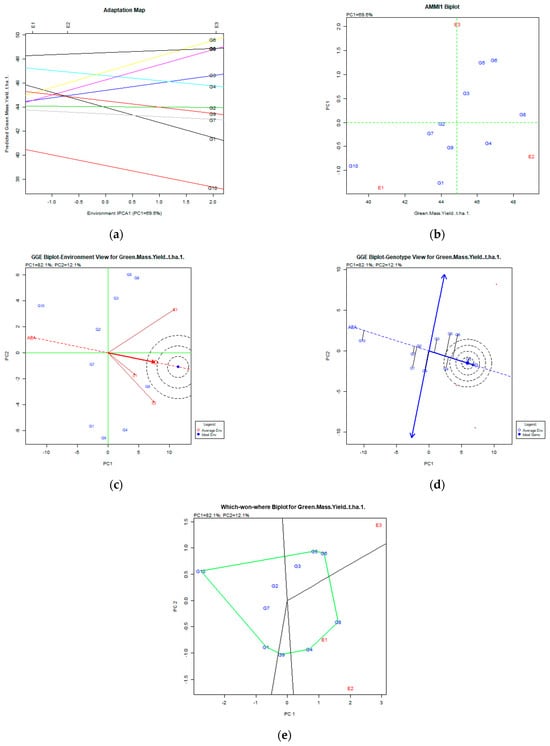
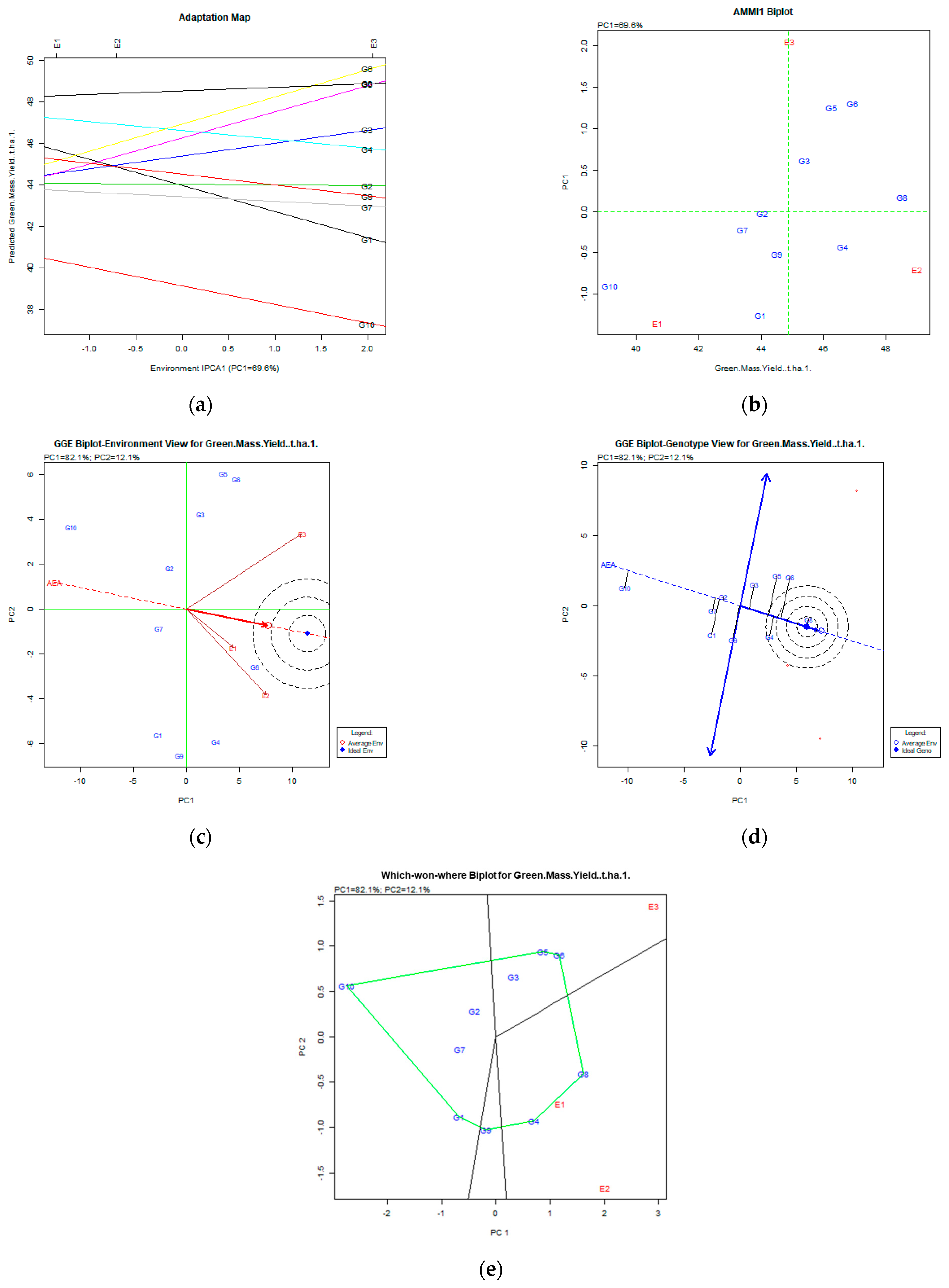
Figure 2.
Green mass yield (t ha−1) stability analysis, based on (a) AMMI adaptation map; (b) AMMI1 biplot; (c) environmental stability GGE biplot; (d) genotypic stability GGE biplot; and (e) which-won-where GGE biplot for specific adaptability of genotypes over environments. The genotypes closer to the ideal genotype are the most desirable.
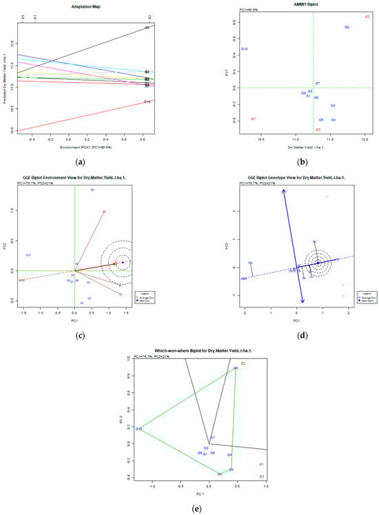
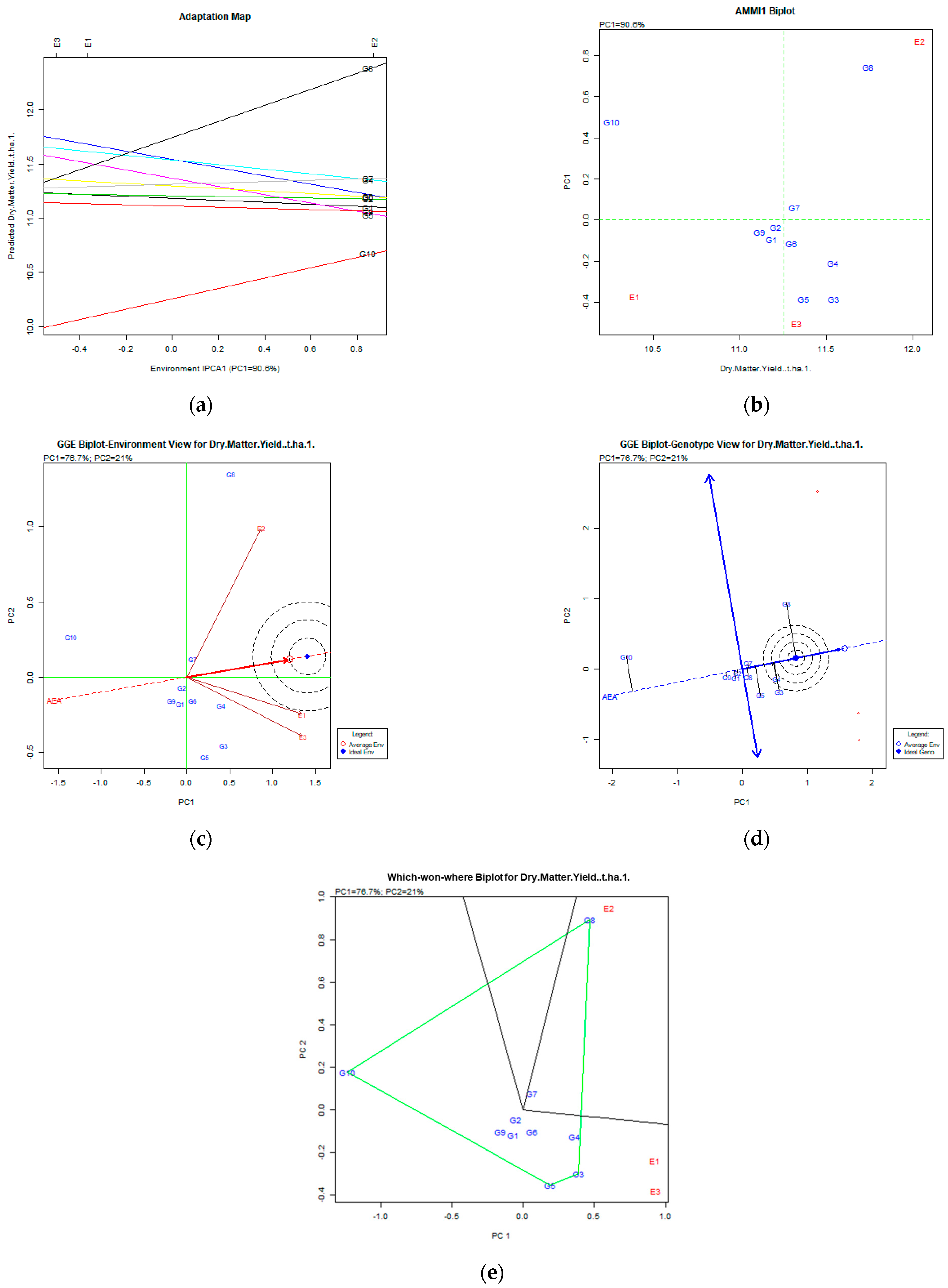
Figure 3.
Dry matter yield (t ha−1) stability analysis based on (a) the AMMI adaptation map; (b) the AMMI1 biplot; (c) the environmental stability GGE biplot; (d) the genotypic stability GGE biplot; and (e) the which-won-where GGE biplot for the specific adaptability of genotypes over environments. The genotypes closer to the ideal genotype are the most desirable.
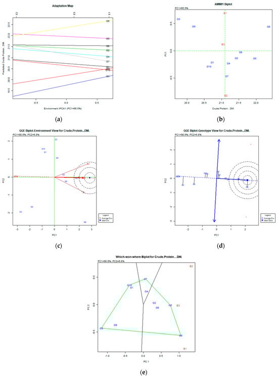
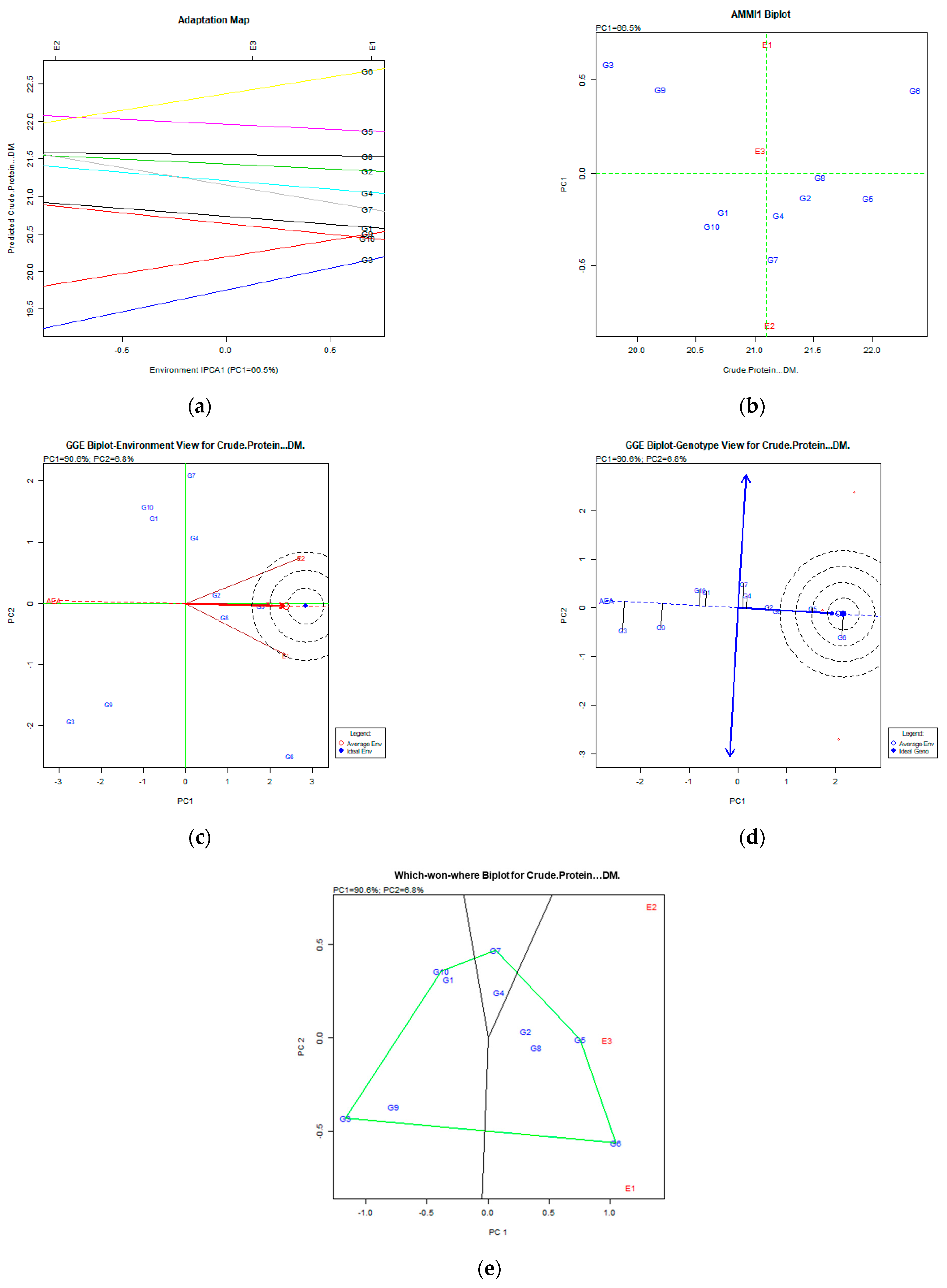
Figure 4.
Crude protein content (%DM) stability analysis based on (a) the AMMI adaptation map; (b) the AMMI1 biplot; (c) the environmental stability GGE biplot; (d) the genotypic stability GGE biplot; and (e) the which-won-where GGE biplot for the specific adaptability of genotypes over environments. The genotypes closer to the ideal genotype are the most desirable.
The AMMI analysis (Figure S1a,b) for the trait of plant height revealed that the G7 (Population 1) was the most stable and desired genotype, since it was placed on the right part of the X axis (the axis of trait) and had a low PC1 value, followed by the G5 (Chaironia), G2 (Dolichi), G4 (Ypati 84), and G1 (Florina). The variation captured by the model for PC1 was 77.9% of the original total variation. The GGE biplot revealed that the G7 (Population 1), G2 (Dolichi), G5 (Chaironia), G4 (Ypati 84), and G1 (Florina) genotypes were the most desirable for stability, since they were placed in the concentric area of stability and adaptability of the bipolot graphic (Figure S1d of biplot of genotypes view). The GGE analysis explained about 98.8% of the total variability (PC1 89.2%, PC2 9.6%). The G7 (Population 1), G5 (Chaironia), G2 (Dolichi), and G4 (Ypati 84) were adapted to environments E1 (2007) and E3, and the which-won-where biplot (Figure S1e) showed that the G7 (Population 1), G5 (Chaironia), G2 (Dolichi), and G4 (Ypati 84) were adapted to environments E1 (2007) and E3 (2009), whereas the G1 (Florina) was adapted to E2 (2008).
AMMI analysis of the trait number of nodes (Figure S2a,b) showed that the variation captured for PC1 (stability) was 68.4% of the total variation and the most stable genotypes were the G4 (Ypati 84) followed by the G2 (Dolichi), G7 (Population 1), and G8 (Population 2), since they were placed in the right part of the X axis combined with low PC1 values. The GGE analysis explained an 80.1% (PC1 65%, PC2 25.1%) of total variability. The desirable genotypes over all environments were the G4 (Ypati 84), followed by the G2 (Dolichi) and G7 (Population 1), since they were placed in the concentric area of stability and adaptability of the biplot (Figure S2d). All environments show high variability (Figure S2c). The which-won-where biplot (Figure S2e) showed that the G1 (Florina) genotype seems to be better adapted to the environment E1 (2007), whereas the G4 (Ypati 84), G7 (Population 1), and G2 (Dolichi) are better adapted in E2 (2008) and E3 (2009) environments.
After the AMMI stability analysis involving the green mass yield (Figure 2a,b), results showed that the most stable genotypes for all environments were the G8 (Population 2), followed by G6 (Chloi), G5 (Chaironia), G4 (Ypati 84), and G3 (Yliki), since they were placed in the right part of the X axis combined with low PC1 values. The PC1 was 69.6%, quite high for acceptable results. Following the GE biplot (Figure 2d), the most stable and productive genotypes were the G8 (Population 2) followed by G4 (Ypati 84). The variability expressed by the GGE biplot analysis for stability and adaptability was 94.2% (PC1 82.1% and PC2 12.1%). All mentioned genotypes were placed near the ideal genotype. The environments expressed high variability (Figure 2c). Genotypes G4 (Ypati 84) and G8 (Population 2) adapted better in E1 (2007) and E2 (2008) environments, and the G5 (Chaironia), G6 (Chloi), and G3 (Yliki) in the E3 (2009) environment (which-won-where biplot Figure 2e).
AMMI analysis of dry matter yield (Figure 3) showed that the variation captured was 90.6% of the original total variability, and the stable and desirable genotypes were G8 (Population 2), followed by G4 (Ypati 84), and G3 (Yliki). For the trait of dry matter, the G8 was the most productive and unstable, followed by more stable but less productive G4 and G3 genotypes for both AMMI and GGE biplots.
However, we have to take into account that green mass and dry matter have a high and significant coefficient of correlation of 0.795. For this instability, it is not clear why, but it is commonly expected that high green mass also means high dry matter yield. Taking into account all the above, the G8 population, even if it is unstable, is an interesting genotype for selection, taking into account the performance of the other traits.
On the other hand, according to the GGE biplot, the stable genotypes for dry matter were G8, followed by G4 (Ypati 84) and G3 (Yliki), since they were placed in and near the concentric area of the desirable genotypes (Figure 3d). The variability for stability and adaptability explained was 97.7% (PC1 76.7% and PC2 21%). The environments were quite diverse as the diagram revealed in Figure 3e: G8 (Population 2) adapted to the E2 (2008) environment, whereas the G3 (Yliki), G4 (Ypati 84), and G5 (Chaironia) adapted to the E1 (2007) and E3 (2009) environments.
Regarding the crude protein content trait (Figure 4a,b), the analysis on AMMI captured 66.5% of the total variation and classified genotypes based on their stability as follows: G5 (Chaironia), G8 (Population 2), G2 (Dolichi), and G6 (Chloi), since they were placed in the right position of the X axis and had low PC1 values. The GGE biplot analysis revealed that the desired genotypes were G6 (Chloi), G5 (Chaironia), and G8 (Population 2) since they were placed in and near the concentric area of the desirable genotypes. The portion of the total variability of stability and adaptability explained was 97.4% (PC1 60.6% and PC2 6.8%—Figure 4c,d). The which-won-where biplot (Figure 4e) showed that the G6 (Chloi) adapted better to the E1 environment and the G5 (Chaironia), G2 (Dolichi), and G8 (Population 2) to E3 (2009).
The AMMI analysis captured 71.4% of the total variation for the crude fiber trait (Figure S3) showing G3 (Yliki), G6 (Chloi), and G2 (Dolichi) (Figure S3a,b) as the most desirable genotypes. The GGE biplot analysis explained about 96.4% of the total variability (PC1 88.7% PC2 7.7%) and revealed G3 (Yliki), G6 (Chloi), and G2 (Dolichi) as the most stable genotypes in all environments. The environments expressed quite low variability for this trait. According to the which-won-where biplot (Figure S3e), the G3 (Yliki), G6 (Chloi), and G2 (Dolichi) adapted better to E1 (2007) and E3 (2009) environments.
Regarding the ash content (Figure S4), the AMMI analysis showed that the PCA captured 71.4% of the total variability, and both the adaptation map (Figure S4a) and AMMI1 (Figure S4b) showed that the G3 (Yliki) genotype, followed by G6 (Chloi) and G2 (Dolichi), were the most stable and most productive for this trait since they were productive combined with low PC1 values. The GGE biplot showed that the environments were quite stable and the genotype view biplot (Figure S4d) showed that the productivity and stability of genotypes decreased in the following order: G3 (Yliki), G6 (Chloi), and G2 (Dolichi) (placed in the concentric area of the ideal genotype). The which-won-where biplot (Figure S4e) showed that the genotypes G3 (Yliki) and G6 (Chloi) were adapted well to the E1 (2007) and E3 (2009) environments.
3.5. Exploratory Data Analysis
Cluster analysis was performed to find relationships among the studied alfalfa genotypes and a heat map (Figure 5) was generated. Cluster analysis alone or in combination with principal components analysis is generally used for the classification of various genetic materials (e.g., peas and grapes) [26,57]. Samples from alfalfa genotypes were divided into six groups (noted with different colors: purple, light blue, brown, blue, green, and red) of increasing dissimilarity. A similar composition among the samples within the same group is underlined. It is visible that alfalfa genotypes were divided into two distinct clusters (C1 and C2), each one having three subclusters (SC1, SC2, and SC3, and SC4, SC5, and SC6, respectively). Grouping for each subcluster revealed that there exists differences among alfalfa cultivations. More specifically, SC1 (purple) consisted of the Population 3 genotype, which was characterized by a lower crude protein, crude fiber, ash content, number of nodes, and plant height. SC2 (light blue) consisted of the Chloi genotype with lower crude fiber, number of nodes, and plant height, but high protein content and intermediate-to-high ash content. SC3 (brown) consisted solely of the Yliki genotype, characterized by lower crude protein, number of nodes, and plant height, but a high content of ash, protein, and intermediate-to-high content of crude fiber. SC4 (dark blue) included various other subgroups, which had intermediate plant height and ash content with two distinct subgroups, one with high and one with lower crude fiber content. SC5 (green) contained various other subgroups of genotypes with lower ash content and higher crude fiber and plant height. Lastly, SC6 (red) included genotypes exhibiting higher plant height, low green mass yield, and dry matter yield.
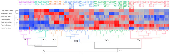
Figure 5.
Heatmap of correlations based on the variables measured in alfalfa using Ward’s method on the standardized data to define distances between clusters. The color of the square areas in the map dendrogram gradually changes from blue that indicates low values to red that indicates high values. OIK 1 to 4 correspond to population 1 to 4.
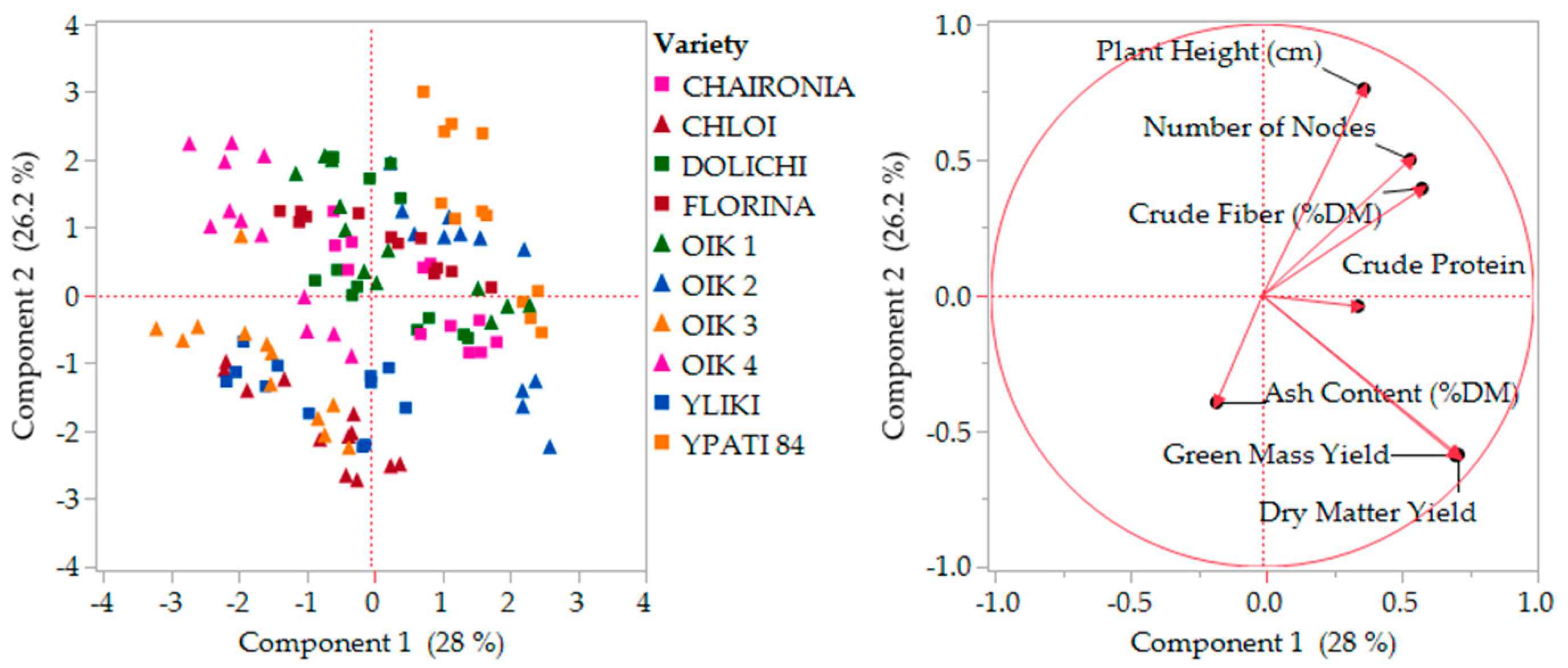
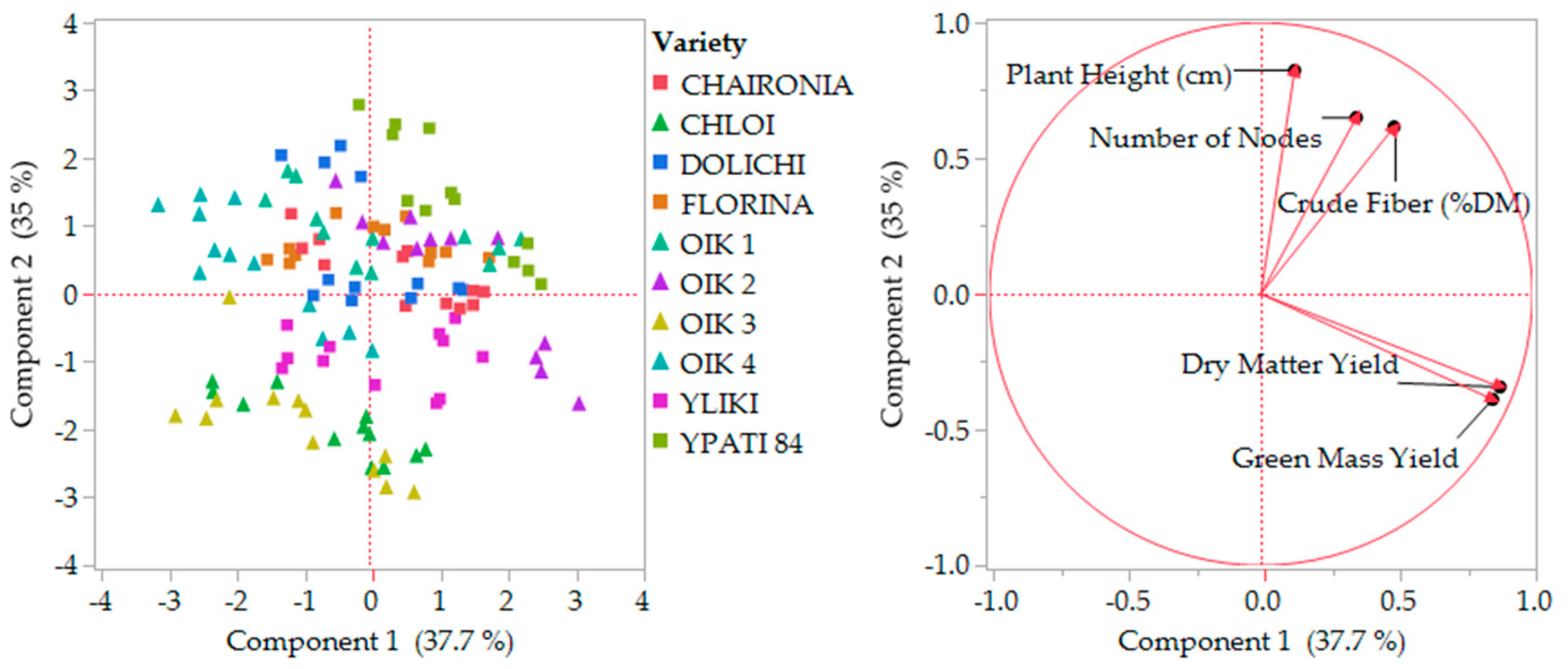
The principal components analysis was performed and scaled in two stages (1. All the characteristics and 2. By missing the less relevant), in order to determine variability and characteristics’ contribution, as presented in Figure 6 and Figure 7. Stage one explained almost 55% of variability by two main coordinates, and stage two explained 73% of variability by missing ash content, which showed slightly different behavior. The distribution of varieties did not change considerably.
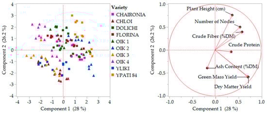
Figure 6.
First stage component analysis with all characteristics. OIK 1 to 4 correspond to population 1 to 4.
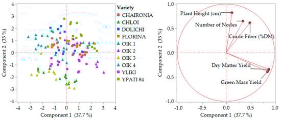
Figure 7.
Second stage component analysis by missing ash content. OIK 1 to 4 correspond to population 1 to 4.
4. Discussion
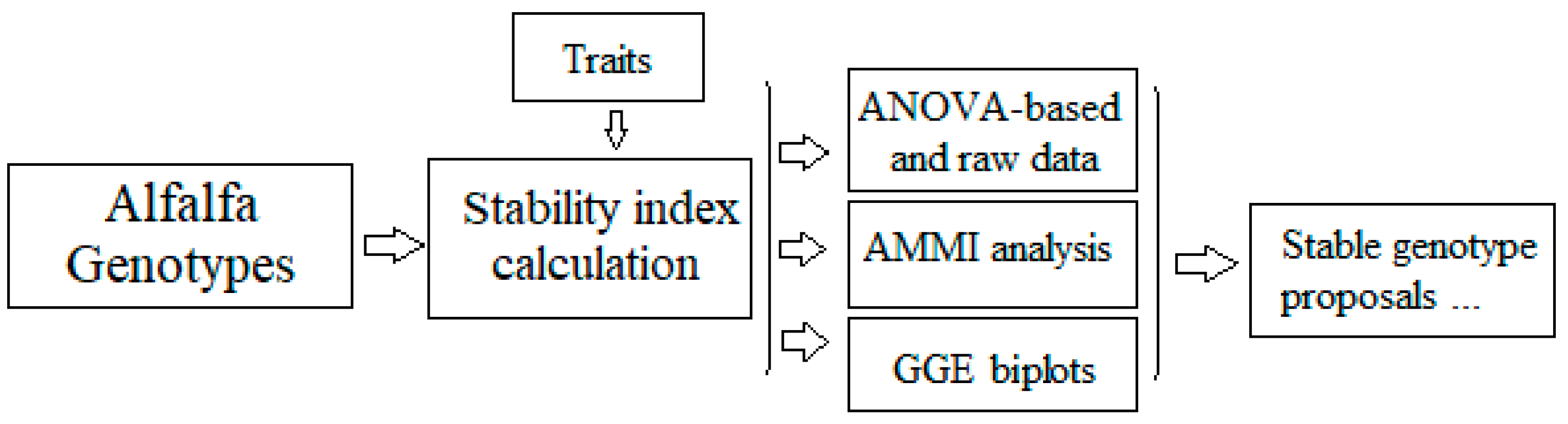
The final scheme of stability analysis is described in Figure 8. The stability index is calculated for all traits of alfalfa. Then, a combined analysis involving raw data, ANOVA, AMMI, and GGE biplot is performed in order to define the most stable traits and the better genotypes exhibiting stability for these traits. Consequently, according to the specific environmental conditions, the best (ideal) genotype that matched the certain conditions was revealed.
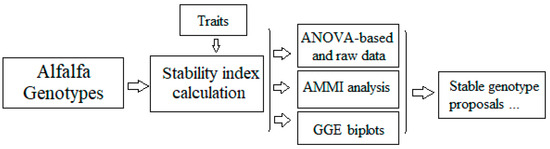
Figure 8.
A model of analyzing trait stability in alfalfa.
According to the ANOVA table, G × E interactions were highly significant in our research. Greveniotis et al. [24,25,26,27,46,47] reported that G × E interactions often occur in the cultivations of many plants aiming to support livestock, meaning different behavior in different places or years. The main traits of alfalfa breeders and farmers, taking into account green mass yield, dry matter yield, and protein content (%), are subjective to GEI [5]. Metochis and Orphanos [58] and Tucak et al. [59] reported differentiated yielding behavior in alfalfa according to environmental conditions or the origin of cultivars [4]. Using molecular markers and clustering, Alzahrani et al. [4] managed to separate cultivars into two groups, according to the usefulness in a breeding program of alfalfa: that is, to produce varieties more drought-tolerant and high-yielding. Also, Sayed et al. [15] reported different behaviors of alfalfa genotypes due to genetic differences and the year of the experiment for the yield, crude protein %, crude fiber %, and ash %.
In our study, crude fiber (%) showed the greatest stability index that exceeded 10,000 for five genetic materials, whereas crude protein content (%) also showed high values for three genetic materials. The third qualitative trait, ash content, also showed high values. For breeders, using the appropriate breeding technique requires an understanding of the qualitative or quantitative inheritance of traits. According to Fasoulas [60], qualitative inheritance is linked to both extensive trait stability and a modest number of genes governing a trait. Greveniotis et al. [27,46,47] claim that qualitative characteristics also show high stability indices. According to Fasoulas [60], the low stability index values suggest a somewhat unstable behavior brought on by quantitative inheritance and multi-gene activity. Nevertheless, plant height is considered a quantitative trait with high values. Green mass yield showed the lowest values, and variety Dolichi together with Population 4 showed the highest values for green mass. Dolichi, Ypati 84, and Yliki showed the highest values for dry matter yield.
All qualitative traits (protein, ash, and fiber content) showed high heritability values based on the stability index and over 90%, as reported by Greveniotis et al. [27,46] in other cultivations. Yield stability indices have acceptable levels concerning heritability, ensuring that the genotype reflects better in the phenotype, simplifying the identification of promising genotypes by breeders. Sayed et al. [15] reported high estimates for GCV% and PCV%, but these values do not always follow high heritability estimates, indicating the presence of genetic variability and effective potential selection for the traits studied. These findings were in agreement with our results and nevertheless, our results were based on stability estimates of certain characteristics after calculating stability indices and not on per se measurements of these characteristics. It seems that stability may ensure high heritability, after successful breeding for the characteristics studied, as a consequence of a proper breeding procedure. This remark may be useful to breeders who develop genetic materials to be used as potential cultivars, providing farmers with high-quality seeds that will exhibit high and stable performance.
Significant correlations were found between crude protein content and green mass yield. This suggests that, although not always linearly, high protein content stability can be ensured by high green mass yield stability, and vice versa. Also, the trait number of nodes strongly correlated to plant height, crude protein, and crude fiber content. Greveniotis et al. [27] proposed that correlations between qualitative traits and yield components may be useful for indirect selection in order to accelerate breeding procedures. Afsharmanesh [61] reported that alfalfa’s dry matter yield highly correlates with the traits of plant height, stem number/unit area, and leaf area index. Although plant height was used as a selection criterion to obtain superior genotypes at early stages [62], in the present study, there was no correlation between plant height and yield in the case of the stability of performance. Takawale et al. [63] reported significant correlations between the following traits of alfalfa: green mass yield was significantly correlated to plant height, tillers per plant to internodal length, dry matter yield to plant height, tillers per plant, and internodal length and crude protein yield. Yield to crude protein content is in agreement with our findings, but breeding for yield must include the parameter of the increasing number of nodes.
AMMI and GGE analysis revealed the G8 (Population 2) genotype as the most productive and acceptably stable across all environments for all traits, followed by G6 (Chloi), G5 (Chaironia), and G2 (Dolichi). Both analyses showed, more or less, the same genotypes as stable and desirable. The AMMI tool was successfully used by Temesgen et al. [64] to define the most adaptable genotypes for specific environments, while Gurmu et al. [65] utilized the GGE biplot to define the most adaptive faba beans cultivars.
In the present study, the statistical elaboration of the results with the abovementioned tools revealed that genotype was an important factor affecting yield. In the case of alfalfa under Mediterranean conditions, GGE biplot analysis discriminated genotype types according to biomass yield, or total yield, and those having high adaptability for both traits [15]. These literature findings indicate that stability analysis of our genotypes under different environmental conditions is fundamental to distinguishing the most adaptable cultivars for cultivating or breeding purposes. GGE analysis discriminated the obtained data better than AMMI; thus, we suggest using it when discovering the best genotypes suited for a specific environment.
Successful grouping of genetic materials was performed by using certain selected traits. Differently, the principal component analysis also resulted in variety distribution, where ash content showed a negative contribution. By excluding that characteristic, the variability explanation reached 73%. Maybe this is due to the total ingredient content of the materials used and must be analyzed further because of the consequences on animal nutrition.
5. Conclusions
In different environments, the stability of performance has more importance than the performance per se. Our approach for modeling the stability of alfalfa involved stability index measurements, genetic parameter calculations, and statistical tools, including cluster analysis, AMMI, and GGE. Interactions G × E were statistically significant for all traits studied. Dolichi and Population 4 showed the highest stability values for green mass. Ypati 84, Yliki, and Dolichi showed the highest stability values for dry matter yield. According to genetic parameters, all qualitative traits (protein, ash, and fiber content) showed high heritability. Yield stability indices were at a satisfactory level. Correlations showed a significant relationship between green mass yield and crude protein content, which means high yield stability may ensure high protein content stability and the opposite, under certain environmental and breeding conditions.
The AMMI and GGE analysis revealed that the optimal genotypes to utilize are the G8 (Population 2) followed by cultivars G6 (Chloi), G5 (Chaironia), and G2 (Dolichi) for all traits. The results of the present study revealed that the GGE biplot is an efficient tool for identifying adaptable and stable cultivars. These findings can be used to make the best choice in terms of cultivars and the populations of alfalfa that best fit a specific environment.
Supplementary Materials
The following supporting information can be downloaded at https://www.mdpi.com/article/10.3390/agriculture14040542/s1, Figure S1. Plant height (cm) stability analysis, based on (a) AMMI adaptation map; (b) AMMI1 biplot; (c) Environmental stability GGE biplot; (d) Genotypic stability GGE biplot; (e) Which-won-where GGE biplot for specific adaptability of genotypes over environments. The genotypes closer to the ideal genotype are the desirable. Figure S2. Number of nodes stability analysis, based on (a) AMMI adaptation map; (b) AMMI1 biplot; (c) Environmental stability GGE biplot; (d) Genotypic stability GGE biplot; (e) Which-won-where GGE biplot for specific adaptability of genotypes over environments. The genotypes closer to the ideal genotype are the desirable. Figure S3. Crude fiber content (%DM) stability analysis, based on (a) AMMI adaptation map; (b) AMMI1 biplot; (c) Environmental stability GGE biplot; (d) Genotypic stability GGE biplot; (e) Which-won-where GGE biplot for specific adaptability of genotypes over environments. The genotypes closer to the ideal genotype are the desirable. Figure S4. Ash content (%DM) stability analysis, based on (a) AMMI adaptation map; (b) AMMI1 biplot; (c) Environmental stability GGE biplot; (d) Genotypic stability GGE biplot; (e) Which-won-where GGE biplot for specific adaptability of genotypes over environments. The genotypes closer to the ideal genotype are the desirable.
Author Contributions
Conceptualization, V.G. and S.Z.; methodology, V.G. and S.Z.; investigation, V.G., C.G.I., D.K. and E.B.; statistical analysis, A.S., A.K. and V.G., writing—original draft preparation, V.G., E.B., A.K. and C.G.I.; writing—review and editing, A.S., V.G. and E.B.; visualization, A.S., A.K. and V.G.; supervision, V.G.; project administration, V.G. All authors have read and agreed to the published version of the manuscript.
Funding
This research received no external funding.
Data Availability Statement
The datasets utilized in this study’s analysis are available upon reasonable request.
Conflicts of Interest
The authors declare no conflicts of interest.
References
- Richard, C. Utilising Lucernes potential for dairy farming. In Proceedings of the 18th International Farm Managment Congress, Methven, Canterbury, New Zealand, 20–25 March 2011; pp. 227–235. [Google Scholar]
- Rojas-Garcia, A.; Torres-Salado, N.; Joaquin-Cancino, S.; Hernandez-Garay, A.; Maldonado-Peralta, M.; Sanchez-Santillan, P. Yield Components of Alfalfa (Medicago sativa L.) Varieties. Agrociencia 2017, 51, 697–708. [Google Scholar]
- Atumo, T.T.; Kauffman, R.; Talore, D.G.; Abera, M.; Tesfaye, T.; Tunkala, B.Z.; Zeleke, M.; Kalsa, G.K. Adaptability, forage yield and nutritional quality of alfalfa (Medicago sativa) genotypes. Sustain. Environ. 2021, 7, 1895475. [Google Scholar] [CrossRef]
- Alzahrani, O.R.; Alshehri, M.A.; Alasmari, A.; Ibrahim, S.D.; Oyouni, A.A.; Siddiqui, Z.H. Evaluation of genetic diversity among Saudi Arabian and Egyptian cultivars of alfalfa (Medicago sativa L.) using ISSR and SCoT markers. J. Taibah Univ. Sci. 2023, 17, 2194187. [Google Scholar] [CrossRef]
- Liatukienė, A.; Norkevičienė, E.; Danytė, V.; Liatukas, Ž. Diversity of Agro-Biological Traits and Development of Diseases in Alfalfa Cultivars during the Contrasting Vegetation Seasons. Sustainability 2023, 15, 1445. [Google Scholar] [CrossRef]
- Yüksel, O.; Albayrak, S.; Türk, M.; Sevimay, C.S. Dry matter yields and some quality features of alfalfa (Medicago sativa L.) cultivars under two different locations of Turkey. J. Ant. Appl. Sci. 2016, 20, 155–160. [Google Scholar] [CrossRef]
- Geren, H.; Kir, B.; Demiroglu, G.; Kavut, Y.T. Effects of different soil textures on the yield and chemical composition of alfalfa (Medicago sativa L.) cultivars under Mediterranean climate conditions. Asian J. Chem. 2009, 21, 5517. [Google Scholar]
- Sommer, A.; Vodnansky, M.; Petrikovic, P.; Pozgaj, R. Influence of Lucerne and meadow hay quality on the digestibility of nutrients in the roe deer. Czech J. Anim. Sci. 2005, 50, 74–80. [Google Scholar] [CrossRef]
- Horvat, D.; Viljevac Vuletić, M.; Andrić, L.; Baličević, R.; Kovačević Babić, M.; Tucak, M. Characterization of Forage Quality, Phenolic Profiles, and Antioxidant Activity in Alfalfa (Medicago sativa L.). Plants 2022, 11, 2735. [Google Scholar] [CrossRef] [PubMed]
- Fahad, S.; Bajwa, A.A.; Nazir, U.; Anjum, S.A.; Farooq, A.; Zohaib, A.; Sadia, S.; Nasim, W.; Adkins, S.; Saud, S. Crop production under drought and heat stress: Plant responses and management options. Front. Plant Sci. 2017, 8, 1147. [Google Scholar] [CrossRef] [PubMed]
- Kebede, G.; Assefa, G.; Feyissa, F.; Mengistu, A.; Tekletsadik, T.; Minta, M.; Tesfaye, M. Biomass yield potential and herbage quality of alfalfa (Medicago sativa L.) genotypes in the central highland of Ethiopia. Int. J. Res. Stud. Agric. Sci. 2017, 3, 14–26. [Google Scholar]
- Odeseye, A.O.; Amusa, N.A.; Ijagbone, I.F.; Aladele, S.E.; Ogunkanmi, L.A. Genotype by Environment Interactions of Twenty Accessions of Cowpea [Vigna unguiculata (L.) Walp.] across Two Locations in Nigeria. Ann. Agrar. Sci. 2018, 16, 481–489. [Google Scholar] [CrossRef]
- Wayu, S.; Atsbha, T. Evaluation of dry matter yield, yield components and nutritive value of selected alfalfa (Medicago sativa L.) cultivars grown under Lowland Raya Valley, Northern Ethiopia. Afr. J. Agrc. Res. 2019, 14, 705–711. [Google Scholar]
- Avci, M.A.; Ozkose, A.; Tamkoc, A. Determination of yield and quality characteristics of alfalfa (Medicago sativa L.) varieties grown in different locations. J. Anim. Vet. Adv. 2013, 12, 487–490. [Google Scholar]
- Sayed, M.R.I.; Alshallash, K.S.; Safhi, F.A.; Alatawi, A.; Alshamrani, S.M.; Dessoky, E.S.; Althobaiti, A.T.; Althaqafi, M.M.; Gharib, H.S.; Shafie, W.W.M.; et al. Genetic Diversity, Analysis of Some Agro-Morphological and Quality Traits and Utilization of Plant Resources of Alfalfa. Genes 2022, 13, 1521. [Google Scholar] [CrossRef]
- Fasoulas, A.C. A moving block evaluation technique for improving the efficiency of pedigree selection. Euphytica 1987, 36, 473–478. [Google Scholar] [CrossRef]
- Kontsiotou, H.; Zotis, S. Variation of characteristics in 21 Greek ecotypes of alfalfa (Medicago sativa L.). In Proceedings of the 5th National Hellenic Conference in Genetics and Plant Breeding, Volos, Greece, 18–20 October 1994; pp. 220–228. [Google Scholar]
- Tavoletti, S.; Capitani, E.; Pierangeli, S. Evaluation of alfalfa populations collected in the Marche region. In Lucerne and Medics for the XXI Century, Proceedings of the XIII Eucarpia Medicago spp. Group Meeting, Perugia, Italy, 13–16 September 1999; Universita di Perugia: Perugia, Italy, 2000; pp. 228–230. [Google Scholar]
- Popovic, S.; Cupic, T.; Grljusic, S.; Tucak, M. Use of variability and path analysis in determining yield and quality of alfalfa. In Breeding and Seed Production for Conventional and Organic Agriculture, Proceedings of the XXVI Meeting of the EUCARPIA Fodder Crops and Amenity Grasses Section, XVI Meeting of the European Association for Research on Plant Breeding (EUCARPIA) Medicago spp. Group joint Meeting, Perugia, Italy, 2–7 September 2006; Universita degli Studi di Perugia—Facolta di Agraria: Perugia, Italy, 2007; pp. 95–99. [Google Scholar]
- Seiam, M.A.; El-Nahrawy, M.A. Selection of some alfalfa populatios for forage yield and quality using modified mass selection. Egypt. J. Plant Breed. 2020, 24, 617–630. [Google Scholar]
- Ünal, S.; Mutlu, Z.; Efe, B. Agromorphological, yield and quality characteristics of two populations of alfalfa developed by mass selection. Cienc. Rural. Santa Maria 2023, 53, e20220036. [Google Scholar] [CrossRef]
- Acharya, J.P.; Lopez, Y.; Gouveia, B.T.; de Bem Oliveira, I.; Resende, M.F.R., Jr.; Muñoz, P.R.; Rios, E.F. Breeding Alfalfa (Medicago sativa L.) Adapted to Subtropical Agroecosystems. Agronomy 2020, 10, 742. [Google Scholar] [CrossRef]
- Eren, B.; Keskin, B.; Demirel, F.; Demirel, S.; Türkoğlu, A.; Yilmaz, A.; Haliloğlu, K. Assessment of genetic diversity and population structure in local alfalfa genotypes using iPBS molecular markers. Genet. Resour. Crop Evol. 2023, 70, 617–628. [Google Scholar] [CrossRef]
- Greveniotis, V.; Bouloumpasi, E.; Zotis, S.; Korkovelos, A.; Ipsilandis, C.G. A Stability Analysis Using AMMI and GGE Biplot Approach on Forage Yield Assessment of Common Vetch in Both Conventional and Low-Input Cultivation Systems. Agriculture 2021, 11, 567. [Google Scholar] [CrossRef]
- Greveniotis, V.; Bouloumpasi, E.; Zotis, S.; Korkovelos, A.; Ipsilandis, C.G. Estimations on Trait Stability of Maize Genotypes. Agriculture 2021, 11, 952. [Google Scholar] [CrossRef]
- Greveniotis, V.; Bouloumpasi, E.; Zotis, S.; Korkovelos, A.; Ipsilandis, C.G. Stability, the Last Frontier: Forage Yield Dynamics of Peas under Two Cultivation Systems. Plants 2022, 11, 892. [Google Scholar] [CrossRef] [PubMed]
- Greveniotis, V.; Bouloumpasi, E.; Zotis, S.; Korkovelos, A.; Kantas, D.; Ipsilandis, C.G. Genotype-by-Environment Interaction Analysis for Quantity and Quality Traits in Faba Beans Using AMMI, GGE Models, and Stability Indices. Plants 2023, 12, 3769. [Google Scholar] [CrossRef] [PubMed]
- Yan, W.; Tinker, N.A. Biplot analysis of multienvironment trial data: Principles and applications. Can. J. Plant Sci. 2006, 86, 623–645. [Google Scholar] [CrossRef]
- Seiam, M.A.; Mohamed, E.S. Forage Yield, Quality Characters and Genetic Variability of some Promising Egyptian Clover Populations. Egyptian. J. Plant Breed. 2020, 24, 839–858. [Google Scholar]
- Baxevanos, D.; Loka, D.; Tsialtas, T. Evaluation of Alfalfa Cultivars Under Rainfed Mediterranean Conditions. J. Agric. Sci. 2021, 159, 281–292. [Google Scholar] [CrossRef]
- Hakl, J.; Mofidian, S.M.A.; Kozova, Z.; Jaromir, S. Estimation of lucerne yield stability for enabling effective cultivar selection under rainfed conditions. Grass Forage Sci. 2019, 74, 687–695. [Google Scholar] [CrossRef]
- Ceccarelli, S. Positive interpretation of genotype by environment interactions in relation to sustainability and biodiversity. In Plant Adaptation and Crop Improvement; Cooper, M., Hammer, G.L., Eds.; CAB International: Wallingford, UK, 1996; pp. 467–486. [Google Scholar]
- Flores, F.; Moreno, M.T.; Cubero, J.I. A comparison of univariate and multivariate methods to analyze G × E interaction. Field Crops Res. 1998, 56, 271–286. [Google Scholar] [CrossRef]
- Elias, A.A.; Robbins, K.R.; Doerge, R.W.; Tuinstra, M.R. Half a century of studying genotype x environment interactions in plant breeding experiments. Crop Sci. 2016, 56, 2090–2105. [Google Scholar] [CrossRef]
- Zobel, R.W.; Wright, M.J.; Gauch, H.G. Statistical analysis of a yield trial. Agron. J. 1988, 80, 388–393. [Google Scholar] [CrossRef]
- Yan, W.; Hunt, L.A.; Sheng, Q.; Szlavnics, Z. Cultivar evaluation and mega-environment investigation based on the GGE biplot. Crop Sci. 2000, 40, 597–605. [Google Scholar] [CrossRef]
- Haile, G.A.; Kebede, G.Y. Identification of Stable Faba Bean (Vicia faba L.) Genotypes for Seed Yield in Ethiopia Using GGE Model. J. Plant Sci. 2021, 9, 163–169. [Google Scholar]
- Fasoula, V.A. Prognostic Breeding: A new paradigm for crop improvement. Plant Breed. Rev. 2013, 37, 297–347. [Google Scholar]
- Steel, R.G.D.; Torrie, H.; Dickey, D.A. Principles and Procedures of Statistics. A Biometrical Approach, 3rd ed.; McGraw-Hill: New York, NY, USA, 1997; p. 666. [Google Scholar]
- Enriquez-Hidalgo, D.; Cruz, T.; Teixeira, D.L.; Steinfort, U. Phenological Stages of Mediterranean Forage Legumes, Based on the BBCH Scale. Ann. Appl. Biol. 2020, 176, 357–368. [Google Scholar] [CrossRef]
- Association of Official Analytical Chemists (AOAC). Official Methods of Analysis of the Association of Official Analytical Chemists, 21st ed.; Oxford University Press: Washington, DC, USA, 2019. [Google Scholar]
- Association of Official Analytical Chemists (AOAC). Official Methods of Analysis, 18th ed.; Association of Official Analytical Chemists (AOAC): Gaithersburg, MD, USA, 2005. [Google Scholar]
- Fasoula, V.A. A novel equation paves the way for an everlasting revolution with cultivars characterized by high and stable crop yield and quality. In Proceedings of the 11th National Hellenic Conference in Genetics and Plant Breeding, Orestiada, Greece, 31 October–2 November 2006; pp. 7–14. [Google Scholar]
- Greveniotis, V.; Fasoula, V.A. Application of prognostic breeding in maize. Crop Pasture Sci. 2016, 67, 605–620. [Google Scholar] [CrossRef]
- Greveniotis, V.; Sioki, E.; Ipsilandis, C.G. Estimations of fiber trait stability and type of inheritance in cotton. Czech J. Genet. Plant Breed. 2018, 54, 190–192. [Google Scholar] [CrossRef]
- Greveniotis, V.; Bouloumpasi, E.; Zotis, S.; Korkovelos, A.; Kantas, D.; Ipsilandis, C.G. A Comparative Study on Stability of Seed Characteristics in Vetch and Pea Cultivations. Agriculture 2023, 13, 1092. [Google Scholar] [CrossRef]
- Greveniotis, V.; Bouloumpasi, E.; Zotis, S.; Korkovelos, A.; Kantas, D.; Ipsilandis, C.G. Stability Dynamics of Main Qualitative Traits in Maize Cultivations across Diverse Environments regarding Soil Characteristics and Climate. Agriculture 2023, 13, 1033. [Google Scholar] [CrossRef]
- McIntosh, M.S. Analysis of Combined Experiments. Agron. J. 1983, 75, 153–155. [Google Scholar] [CrossRef]
- Johnson, H.W.; Robinson, H.E.; Comstock, R.E. Estimate of genetic and environmental variability in soybean. Agron. J. 1955, 47, 314–318. [Google Scholar] [CrossRef]
- Hanson, G.; Robinson, H.F.; Comstock, R.E. Biometrical studies on yield in segregating population of Korean Lespedeza. Agron. J. 1956, 48, 268–274. [Google Scholar] [CrossRef]
- Singh, R.K.; Chaudhary, B.D. Biometrical Methods in Quantitative Genetic Analysis; Kalyani Publishers: New Delhi, India, 1977; p. 304. [Google Scholar]
- Gauch, H., Jr. Statistical Analysis of Regional Yield Trials: AMMI Analysis of Factorial Designs; Elsevier Science Publishers: Amsterdam, The Netherlands, 1992. [Google Scholar]
- Khan, M.M.H.; Rafii, M.Y.; Ramlee, S.I.; Jusoh, M.; Al Mamun, M. AMMI and GGE biplot analysis for yield performance and stability assessment of selected Bambara groundnut (Vigna subterranea L. Verdc.) genotypes under the multi-environmental trials (METs). Sci. Rep. 2021, 11, 22791. [Google Scholar] [CrossRef] [PubMed]
- Koundinya, A.V.V.; Ajeesh, B.R.; Hegde, V.; Sheela, M.N.; Mohan, C.; Asha, K.I. Genetic parameters, stability and selection of cassava genotypes between rainy and water stress conditions using AMMI, WAAS, BLUP and MTSI. Sci. Hortic. 2021, 281, 109949. [Google Scholar]
- Gabriel, K.R. The biplot graphic display of matrices with application to principal component analysis. Biometrika 1971, 58, 453–467. [Google Scholar] [CrossRef]
- Andrade, M.H.M.L.; Patiño-Torres, A.J.; Cavallin, I.C.; Guedes, M.L.; Carvalho, R.P.; Gonçalves, F.M.A.; Marçal, T.D.S.; Pinto, C.A.B.P. Stability of potato clones resistant to potato virus y under subtropical conditions. Crop Breed. Appl. Biotechnol. 2021, 21, e32872118. [Google Scholar] [CrossRef]
- Bouloumpasi, E.; Skendi, A.; Soufleros, E.H. Survey on Yeast Assimilable Nitrogen Status of Musts from Native and International Grape Varieties: Effect of Variety and Climate. Fermentation 2023, 9, 773. [Google Scholar] [CrossRef]
- Metochis, C.; Orphanos, P.I. Alfalfa yield and water use when forced into dormancy by withholding water during the summer. Agron. J. 1981, 73, 1048–1050. [Google Scholar] [CrossRef]
- Tucak, M.; Popovic, S.; Bolaric, S.; Kozumplik, V. Agronomic evaluation of alfalfa genotypes under ecological conditions of eastern croatia. In proceedings of the VII. Alps-Adria Scientific Workshop, 28 April–2 May 2008, Stara Lesna, Slovakia. Part I. Cereal Res. Commun. 2008, 36, 651–654. [Google Scholar]
- Fasoulas, A.C. The Honeycomb Methodology of Plant Breeding; Department of Genetics and Plant Breeding, Aristotle University of Thessaloniki: Thessaloniki, Greece, 1988; p. 168. [Google Scholar]
- Afsharmanesh, G. Study of some morphological traits and selection of drought- resistant alfalfa cultivars (Medicago sativa L.) in Jiroft. Iran. Plant Ecophysiol. 2009, 3, 109–118. [Google Scholar]
- Tucak, M.; Popović, S.; Čupić, T.; Grljušić, S.; Bolarić, S.; Kozumplik, V. Genetic diversity of alfalfa (Medicago spp.) estimated by molecular markers and morphological characters. Period. Biol. 2008, 110, 243–249. [Google Scholar]
- Takawale, P.S.; Jade, S.S.; Bahulikar, R.A.; Desale, J.S. Diversity in Lucerne (Medicago sativa L.) germplasm for morphology, yield and molecular markers and their correlations. Indian. J. Genet. 2019, 79, 453–459. [Google Scholar] [CrossRef]
- Temesgen, T.; Keneni, G.; Sefera, T.; Jarso, M. Yield stability and relationships among stability parameters in faba bean (Vicia faba L.) genotypes. Crop J. 2015, 3, 258–268. [Google Scholar] [CrossRef]
- Gurmu, F.; Lire, E.; Asfaw, A.; Alemayehu, F.; Rezene, Y.; Ambachew, D. GGE-biplot analysis of grain yield of faba bean genotypes in southern Ethiopia. Electron. J. Plant Breed. 2012, 3, 898–907. [Google Scholar]

Disclaimer/Publisher’s Note: The statements, opinions and data contained in all publications are solely those of the individual author(s) and contributor(s) and not of MDPI and/or the editor(s). MDPI and/or the editor(s) disclaim responsibility for any injury to people or property resulting from any ideas, methods, instructions or products referred to in the content. |
© 2024 by the authors. Licensee MDPI, Basel, Switzerland. This article is an open access article distributed under the terms and conditions of the Creative Commons Attribution (CC BY) license (https://creativecommons.org/licenses/by/4.0/).