Abstract
In order to solve the problem of the low pickup efficiency of the robotic arm when harvesting safflower filaments, we established a pickup trajectory cycle and an improved velocity profile model for the harvest of safflower filaments according to the growth characteristics of safflower. Bezier curves were utilized to optimize the picking trajectory, mitigating the abrupt changes produced by the delta mechanism during operation. Furthermore, to overcome the slow convergence speed and the tendency of the ant colony algorithm to fall into local optima, a safflower harvesting trajectory planning method based on an ant colony genetic algorithm is proposed. This method includes enhancements through an adaptive adjustment mechanism, pheromone limitation, and the integration of optimized parameters from genetic algorithms. An optimization model with working time as the objective function was established in the MATLAB environment, and simulation experiments were conducted to optimize the trajectory using the designed ant colony genetic algorithm. The simulation results show that, compared to the basic ant colony algorithm, the path length with the ant colony genetic algorithm is reduced by 1.33% to 7.85%, and its convergence stability significantly surpasses that of the basic ant colony algorithm. Field tests demonstrate that, while maintaining an S-curve velocity, the ant colony genetic algorithm reduces the harvesting time by 28.25% to 35.18% compared to random harvesting and by 6.34% to 6.81% compared to the basic ant colony algorithm, significantly enhancing the picking efficiency of the safflower-harvesting robotic arm.
1. Introduction
Safflower (Carthamus tinctorius L.), indigenous to the eastern Mediterranean, emerges as a versatile cash crop, extensively cultivated for its applications as a medicinal herb, in oil production, for dyes, and as fodder, showcasing remarkable adaptability along with tolerance to cold and heat [1,2]. The harvesting period of safflower primarily spans from July to August, characterized by the asynchronous maturation of safflower filaments, necessitating the selective harvesting of safflower [3,4]. After reaching maturity, within a timeframe of 1–3 days, the water content in safflower filaments diminishes, rendering them dry and brittle. This transformation complicates the harvesting process and precipitates a degradation in the quality of the harvested safflower. It is therefore imperative to complete the safflower harvesting before the filaments become overly desiccated and brittle. Safflower harvesting operations primarily target the collection of mature filaments at the top of the flower heads. A single safflower plant has from four to ten flower heads, arranged in a conical spatial pattern, mainly concentrated at the top of the plant. During the flowering period, safflower capitula progressively blooms from the top of the main stem toward the tops of the peripheral branches. Consequently, optimizing the efficiency of safflower-harvesting robots becomes a critical endeavor [5,6].
There are two commonly used trajectory planning methods to enhance the picking efficiency of safflower-picking robotic arms [7,8]. The first method involves analyzing the motion patterns of individual safflower picking trajectories to ensure smooth path transitions. By maximizing the time it takes for the robotic arm to reach its maximum movement speed, this approach aims to improve picking efficiency. The second method focuses on global path planning for the entire picking path. It determines the optimal sequence of paths for safflower in the region, thereby enhancing the overall efficiency of safflower picking.
The analysis of motion laws represents a significant niche in robotic arm research, contributing to the heightened accuracy of end-effectors and reduced energy expenditure [9,10]. Fang et al. [11] focused on industrial robots used for rapid picking tasks or obstacle avoidance, introducing an improved S-curve speed control method. This significantly enhanced the smoothness of robot operations. However, its implementation is relatively complex, requiring substantial computational resources. Lu et al. [12] delved into minimizing the maximum jerk in the joints of a parallel mechanism, employing various constraints to achieve this goal. However, the complexity of their approach was amplified by the extensive range of factors considered, rendering the process less straightforward.
In the practical context of harvesting, trajectory planning must adhere to the kinematic and dynamic limitations of the robotic arm. This planning phase necessitates a smooth transition between adjacent path points, eliminating sharp inflections. The Bezier curve, rooted in Bernstein polynomials and applied to the mathematical modeling of two-dimensional graphs, is widely adopted for its simplicity and effectiveness in smoothing the appearance of abrupt corners in line segments [13,14]. This technique’s ease of manipulation and ability to refine path aesthetics make it a favored choice in the realm of trajectory planning.
Path planning plays a crucial role in optimizing work efficiency by establishing a more efficient picking order [15,16]. Yao et al. [17] enhanced the state transition strategy of ant algorithms by introducing a weighted guidance function, which provided a more directed approach for the ant agents during their exploration process. Ren et al. [18] improved the local search capabilities of an ant colony algorithm through the implementation of a forbidden search operator, which was informed by a knowledge-based elite strategy and dynamic selection probabilities, thereby enhancing the solution’s precision. This approach emphasized diversifying the learning process to bolster the algorithm’s proficiency in identifying the optimal solution, although further advancements were necessary to improve its convergence. Hu et al. [19] amalgamated an artificial potential field with a logarithmic ant colony algorithm, incorporating factors influencing the potential field into the algorithm’s state transition probabilities and heuristic functions. This integration made the algorithm more directive in pathfinding, thereby hastening its convergence speed. However, this method risked prematurely converging to local optima due to the excessive prioritization of the optimal path.
In order to mitigate the impact of sudden speed changes and long picking paths on the safflower picking process and to improve the overall efficiency of safflower picking, this study proposes a trajectory planning algorithm for safflower-picking robotic arms based on the ant colony genetic algorithm. The algorithm employs a second-order Bezier curve and an improved S-type velocity curve model to optimize the time required for each individual picking path. Additionally, the ant colony genetic algorithm is utilized to plan the picking paths, ensuring the identification of an optimal path sequence and minimizing any negative impact on picking efficiency caused by long paths.
2. Materials and Methods
2.1. Safflower-Picking Robot Working Principle
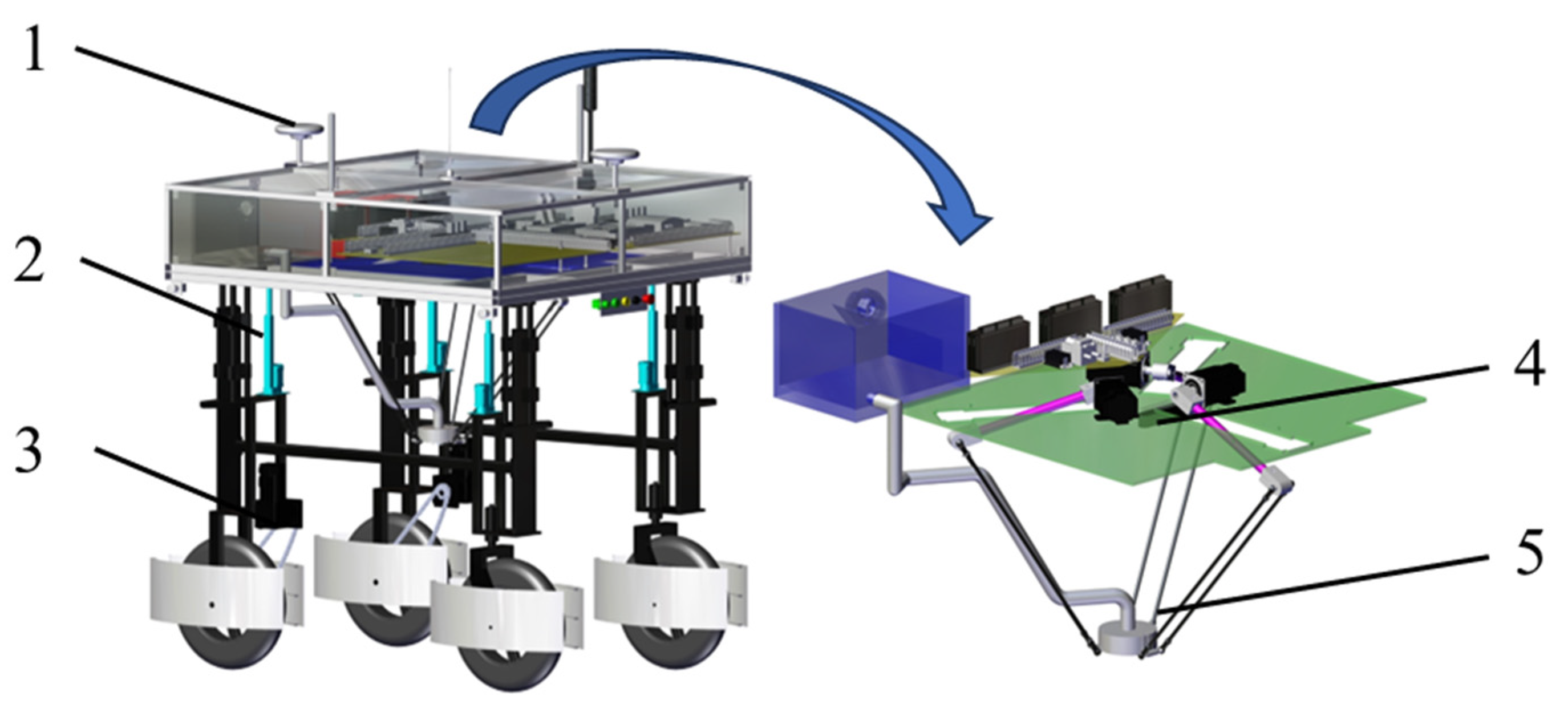
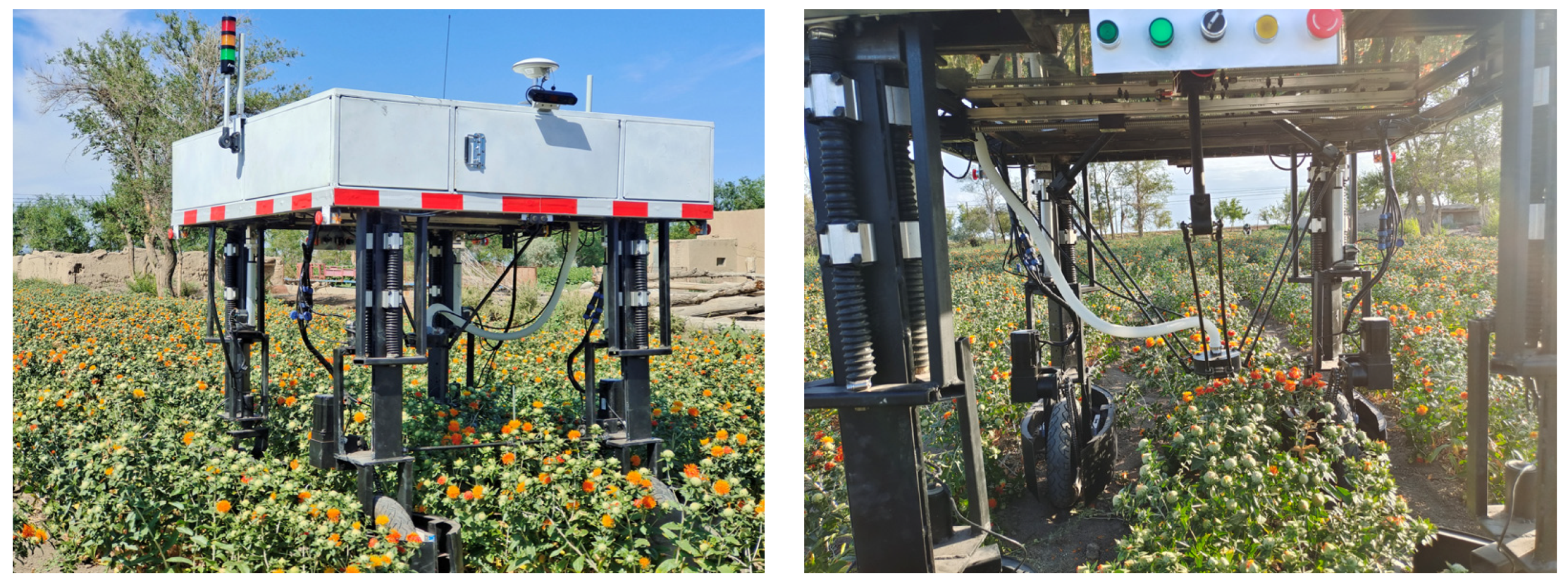
The safflower-picking robot (shown in Figure 1) is mainly composed of a power system, a leveling system, a navigation system, an identification and localization system, and a picking system.

Figure 1.
Main structure of the safflower-picking robot. 1: Navigation system; 2: Leveling system; 3: Power system; 4: Identification and positioning system; 5: Picking system.
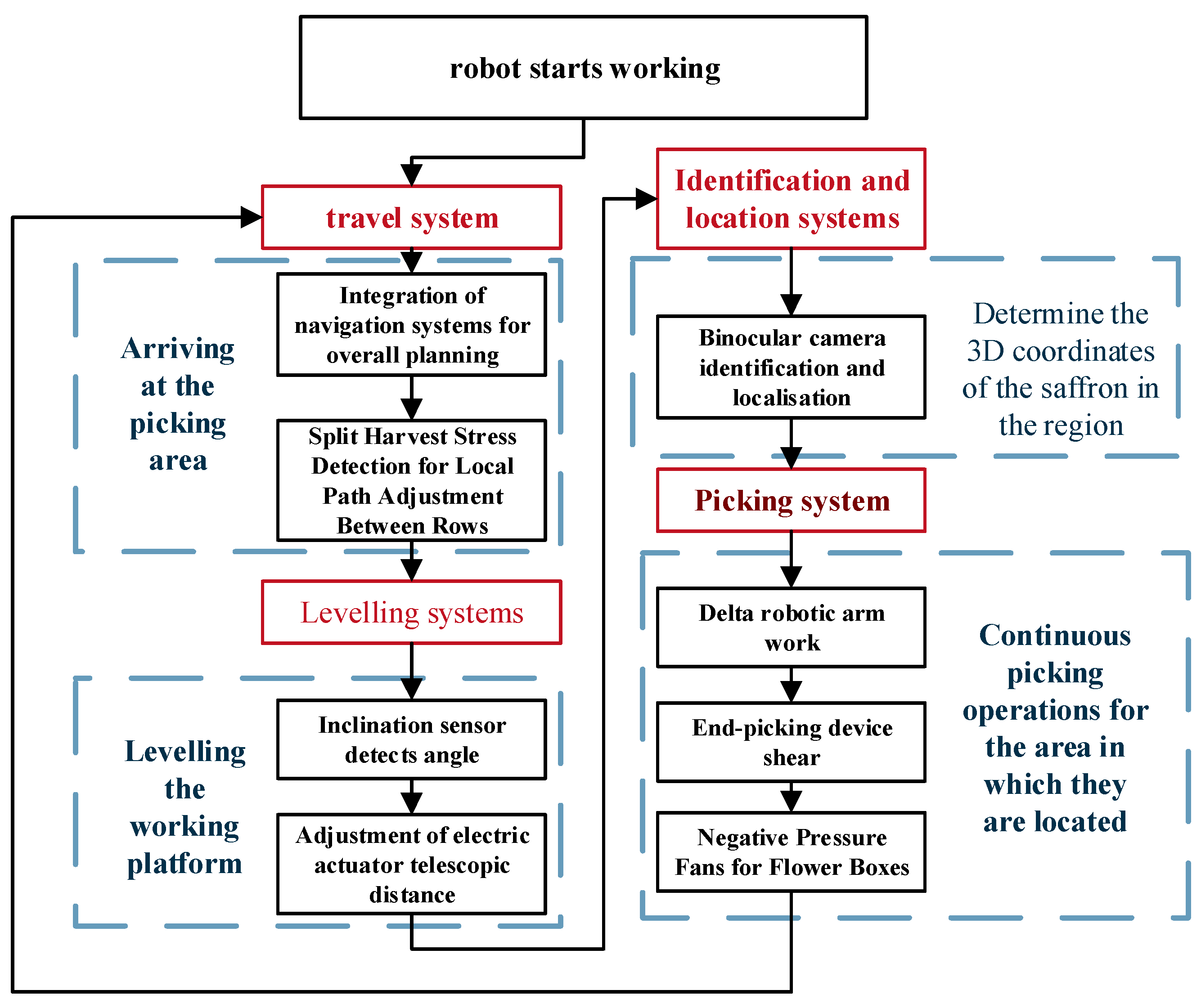
Figure 2 shows the workflow diagram of the whole machine, in which the picking system’s parallel robotic arm operation needs to be in the region of the safflower trajectory planning to reduce its impact and ensure the shortest time possible to pick all the mature safflower in the region.
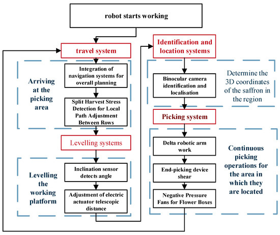
Figure 2.
Workflow diagram of the whole machine.
Figure 2 presents the entire workflow diagram of the machine, wherein the robot’s locomotion system is equipped with integrated navigation technology, achieving precise global positioning and navigation. It also fine-tunes the inter-row path through its pressure detection system to optimize the global navigation route. The robot is fitted with a leveling system that detects the platform’s inclination angle through an inclinometer and automatically adjusts the platform to maintain levelness through the extension and retraction of electric push rods. Furthermore, the identification and location system utilizes binocular cameras and laser imaging detection and ranging (LIDAR) technology to accurately identify and locate the three-dimensional coordinates of mature safflower flowers within the area. The harvesting system, which is the core component of the robot, is responsible for the actual picking tasks. It comprises a robotic arm, an end-effector harvesting device, a flower collection box, and a vacuum fan. The robotic arm plans its trajectory based on the three-dimensional coordinates of mature safflower provided by the identification and location system, ensuring that the harvesting of mature safflower is completed in the shortest time. Meanwhile, the end-effector captures and cuts the safflower, the collection box stores the harvested safflower filaments, and the vacuum fan provides sufficient suction throughout the harvesting process to assist in directing the safflower into the collection box.
2.2. Laws of Motion Analysis
2.2.1. Improved S-Type Velocity Curve Model
The degree of rapidity, also called the rate of change of force, is the rate of change of acceleration, which is an important index for describing the state of motion [20]. An S-type speed curve can limit the degree of rapidity and cause little impact damage to the motor as well as the drive train system. The S-type speed curve can be divided into three parts: the start-up acceleration stage, the maximum speed maintenance stage, and the braking deceleration stage.
The acceleration and deceleration control curve of the parallel arm of the safflower-picking robot should meet the following basic conditions: the acceleration and velocity changes must be smooth and continuous in the whole process, the speed must be consistent with the required velocity at the beginning and the end of the speed change, and the acceleration must be zero. To avoid flexible shock, the degree of urgency must be continuous, i.e., the value at the beginning and end of the acceleration and deceleration positions must be zero. Figure 3 shows the position, velocity, acceleration, and acceleration curve of the whole process of acceleration and deceleration.
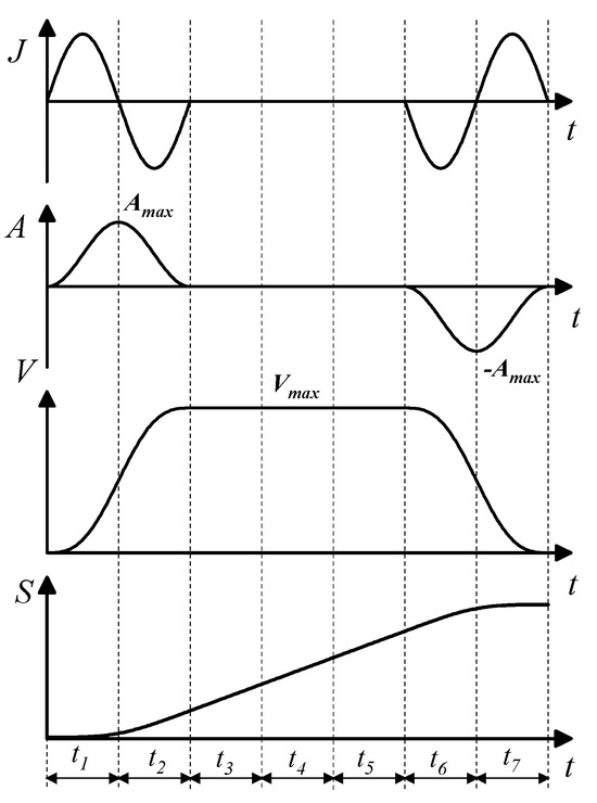
Figure 3.
Characterization of acceleration and deceleration curves. A max signifies the maximum acceleration of the end−effector of the Delta robotic arm, whereas Vmax indicates the maximum speed of the end−effector of the Delta robotic arm. t1 is the time during which acceleration increases during the acceleration phase, t2 is the time during which acceleration decreases during the acceleration phase, t3 to t5 represent the period when the speed is constant at its maximum during the uniform motion phase, t6 is the time during which acceleration increases during the deceleration phase, and t7 is the time during which acceleration decreases during the deceleration phase.
The acceleration process includes acceleration and deceleration, the same as the deceleration process. The acceleration and deceleration are related to each other by uniform velocity. The whole process includes five stages, and the corresponding acceleration and deceleration equations are as follows:
where represents the maximum acceleration at the end of the Delta robotic arm, represents the maximum velocity at the end of the Delta robotic arm, and the starting and ending velocities at the end of the robotic arm are both 0 m/s.
From Figure 3 and Equations (1)–(3), it is evident that, in the accelerating part, the durations t1 and t2 appear to be equal. Similarly, in the decelerating part, the durations t6 and t7 seem to be equal. Taking into account the maximum velocity that the system can reach, denoted as v, we can proceed to calculate the total displacement of the system as follows:
2.2.2. Improved Analysis of Picking Trajectories
This paper identifies a harvesting strategy for safflower filaments tailored to field-picking requirements, maneuvering the robotic arm so its end effector is positioned directly above the safflower filaments. Through precise vertical control, the guide sleeve within the end effector is moved downward to the pre-determined picking point for harvesting safflower filaments. This approach primarily aims to prevent collisions with other flowers on the same plant during the harvesting process, which could alter the target location.
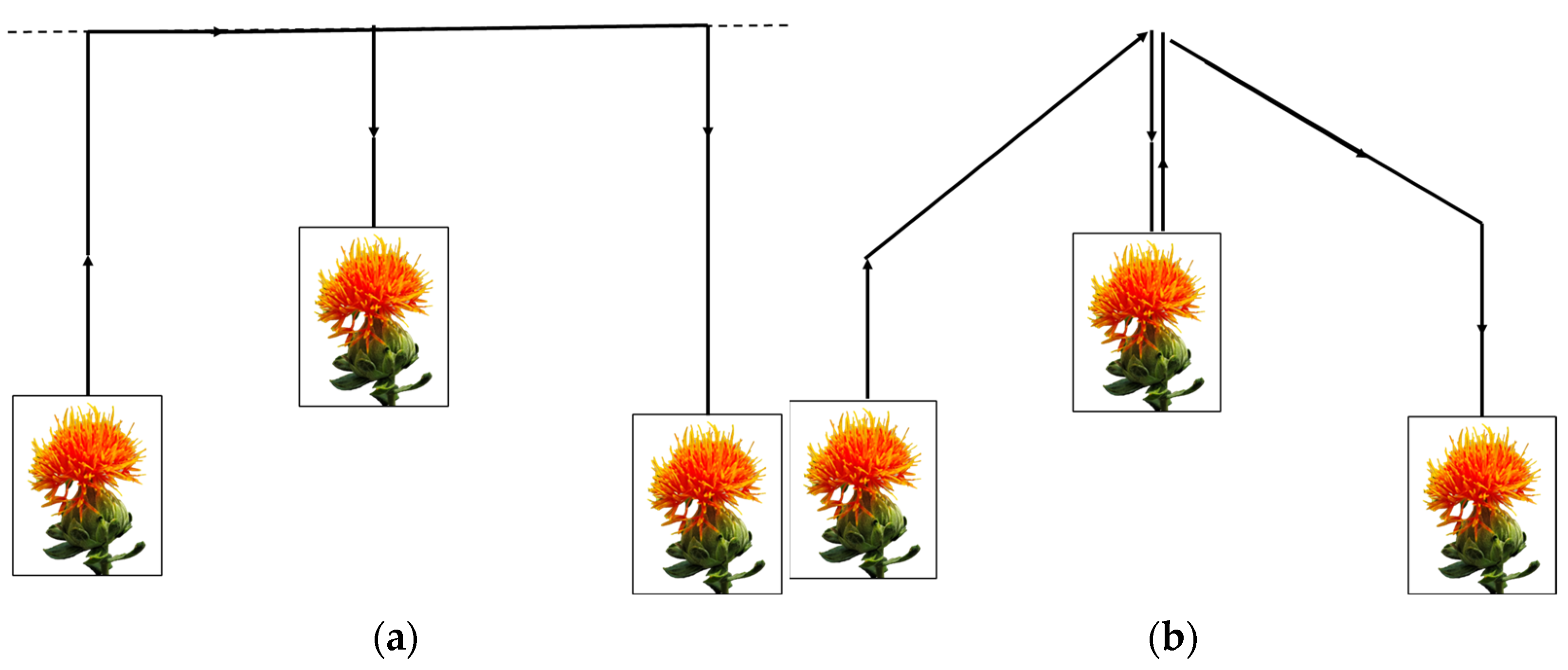
The execution of safflower filament harvesting necessitates the sequential positioning of the end picking device at the targeted, pre-defined locations. Given the likelihood of encountering obstacles such as branches and leaves among the safflowers, establishing a safe descent height becomes essential. Focusing on safflowers situated at varying heights, the conventional movement strategy employed is the gate-type path, as depicted in Figure 4a. Achieving this first requires ensuring that the picking device reaches a safe, uniform height before descending to the targeted location. Although this approach effectively prevents the end effector from impacting safflower filaments mid-movement, it results in an excessively long travel path. To enhance the efficiency of safflower filament harvesting and minimize the travel distance of the end effector while circumventing obstacles, an optimized gate-type path scheme is proposed. This plan ensures that safflower filaments at different elevations maintain a consistent safe height, albeit not at the same level, as illustrated in Figure 4b.
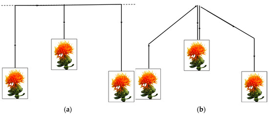
Figure 4.
Motion path: (a) traditional gate-type path; (b) improved gate-type path.
In the field of agricultural automation, such as safflower picking, the utilization of Bezier curves for the trajectory planning of robotic arms can have a significant impact on enhancing operational efficiency and accuracy. By manipulating the control points of the Bezier curve, it becomes possible to effectively plan the trajectory of the robotic arm in complex spatial environments. The incorporation of Bezier curves ensures a seamless and uninterrupted movement of the robotic arm during the safflower-picking process. This smoothness reduces sudden changes and jerking motions, leading to improved overall efficiency when harvesting safflower. Moreover, diminishing fluctuations in the movement of the robotic arm contributes to the preservation of the safflower’s integrity, minimizing any potential damage to the delicate flower and thereby enhancing the accuracy of the picking process.
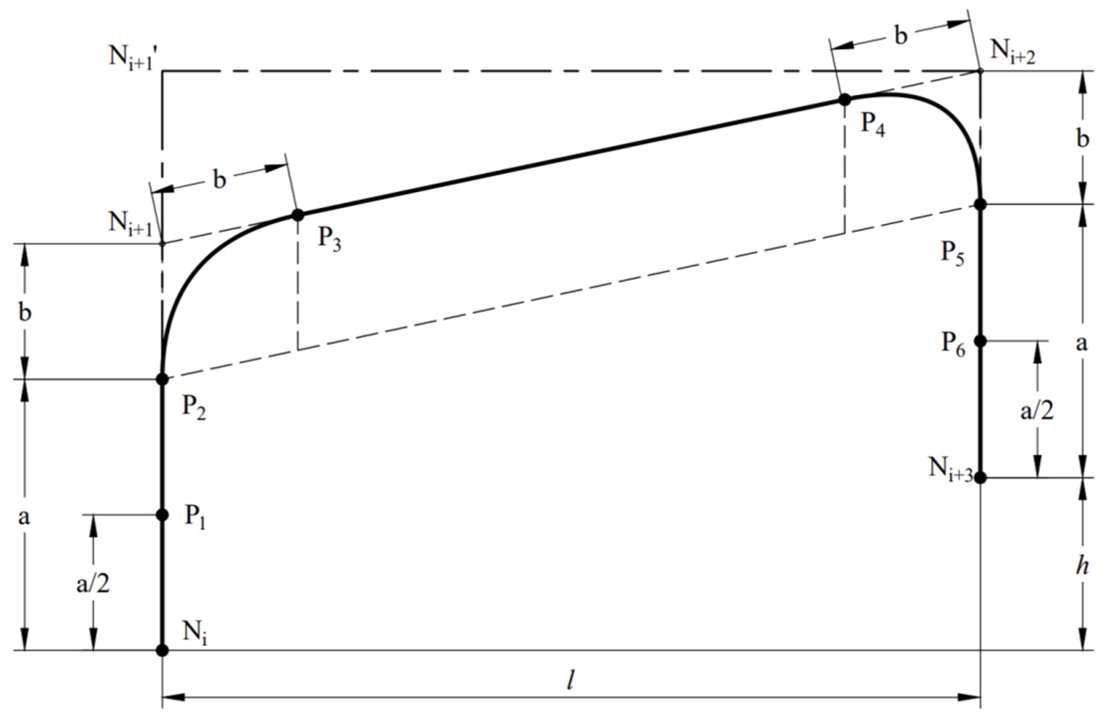
The safflower-picking trajectory cycle starts from the picking point “” and ends at the next picking point “”. As shown in Figure 5, the picking cycle of the safflower-picking robot can be roughly divided into five parts:
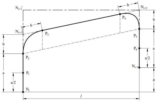
Figure 5.
Cycle diagram of a single trajectory for safflower picking.
- (1)
- The motion accelerates with an increasing acceleration from “” to “”.
- (2)
- The motion continues to accelerate, but with a decreasing acceleration from “” to “”.
- (3)
- After reaching point “”, the motion transitions into a uniform speed or constant velocity motion from “” to “”.
- (4)
- As the motion approaches point “”, it starts to decelerate with an increasing acceleration.
- (5)
- As the motion approaches point “”, it decelerates with a decreasing acceleration until reaching point “”.
To reduce the vibrations from the sudden change in acceleration at the corner and improve the positioning accuracy, Bezier curves are used in the transition section to smooth the transition of the right-angled segments of the “gate”-shaped trajectory, namely “” and “” segments.
The Bezier curve definition is shown in Equation (5):
where is the coordinate information of the ith control point of the line segment and is the Bernstein polynomial, which is the base function of the parametric equation of the Bezier curve.
Here, represents the binomial coefficient, and the equation’s derivative is calculated as follows:
Therefore, the derivative with respect to the points on the Bezier curve can be expressed as follows:
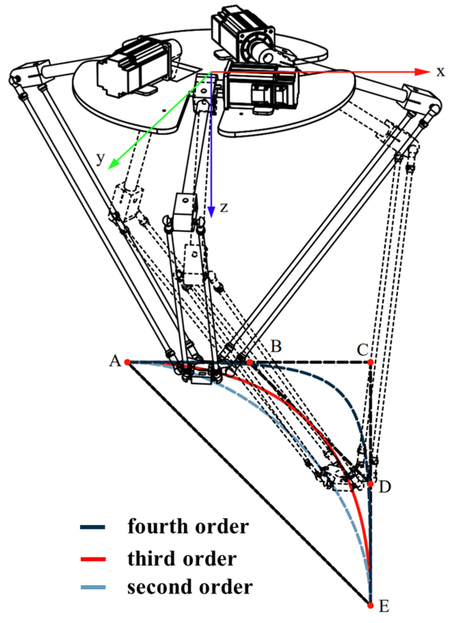
As shown in Figure 6, the second-order Bezier curve is commonly utilized due to its simplicity and efficient handling of single inflection paths. On the other hand, the third-order and fourth-order Bezier curves are not as numerically stable as the second-order Bezier curves, despite offering greater flexibility and control [21]. Therefore, for the smoothing of trajectories in this paper, the second-order Bezier curve is favored.
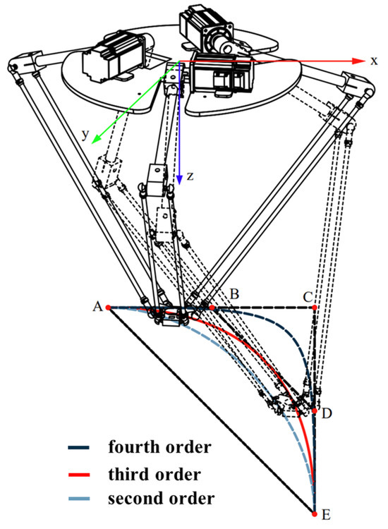
Figure 6.
Bezier curve. where xyz is the static platform coordinate system, A, C, E are second-order Bessel curve reference points, A, B, D, E are third-order Bessel curve reference points, and A, B, C, D, E are fourth-order Bessel curve reference points.
The parametric equations for the points on the second-order Bezier curve can be derived from Equations (5) and (8) as follows:
where , , and are the coordinates of the control points of the second-order Bezier curve.
The curvature, denoted as K(t), of a Bezier curve can be calculated at any given point:
2.3. Improved Ant Colony Genetic Fusion Algorithm
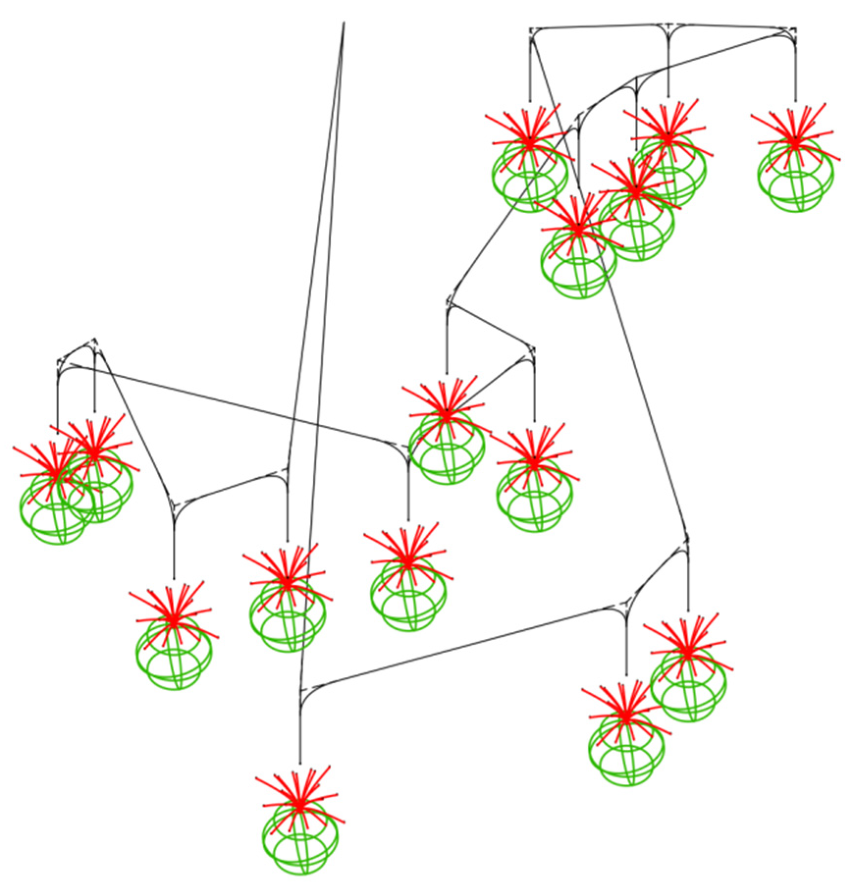
Within the context of the safflower field environment, the distribution of safflower filaments is relatively dense, as depicted in Figure 7a, with the picking locations of safflower filaments dispersed within a three-dimensional space. Amidst a random and chaotic harvesting sequence, the movement path of the terminal picking device is unpredictable, leading to a prolongation of the overall movement trajectory. This, in turn, significantly diminishes the efficiency of the harvesting process. Therefore, it is essential to conduct in-depth research and plan the optimal picking sequence for safflower filaments.
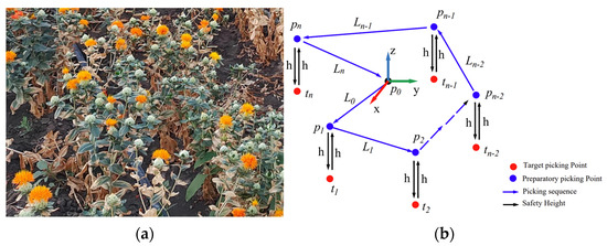
Figure 7.
Schematic diagram of safflower filament harvesting movement: (a) the spatial distribution of harvesting points; (b) the movement pathway for harvesting. Where xyz is the coordinate system of the starting point for trajectory planning.
Figure 7b presents the diagrammatic route of the safflower filament harvesting apparatus, where black dots signify the mechanical arm’s present location and red dots highlight the designated collection sites for the safflower filaments. To ensure that the harvesting mechanism avoids any unintended contact with nearby filaments during operation, establishing a prudent safety elevation is crucial. Blue dots illustrate the safe elevations for the safflower filaments, ensuring that a secure distance is maintained. As depicted, the mechanical arm embarks from its initial position, methodically advances to these secure elevations, and subsequently lowers to the specified harvesting locations at the established safety height for collection. Following the harvest of a specific filament, the arm ascends back to the safe elevation level before continuing to the next designated sites, completing the cycle until all targeted filaments are collected and the device returns to its starting point.
Within a complex three-dimensional space, the ant colony algorithm may become entrapped in local optima or encounter deadlock situations, hindering the arm’s ability to identify the globally optimal path and affecting the overall operational efficiency. The essence of this issue lies in the algorithm’s excessive reliance on local pheromone trails, lacking a sufficient global search mechanism to escape local optima. Deadlock situations arise when the algorithm encounters a state from which it cannot progress, unable to find an effective path to the target location. Given that a three-dimensional environment offers more path choices than a two-dimensional one, it simultaneously increases the complexity and computational demands of the search.
Therefore, in the global path planning for the safflower-harvesting robotic arm, it is necessary to adjust and optimize the ant colony algorithm to enhance its global search capabilities and avoid the problems of local optima, ensuring that the robotic arm can efficiently and accurately complete global path planning and harvesting tasks in the complex environment of safflower harvesting [22,23,24]. The following strategies (Figure 8) should be adopted for optimization.
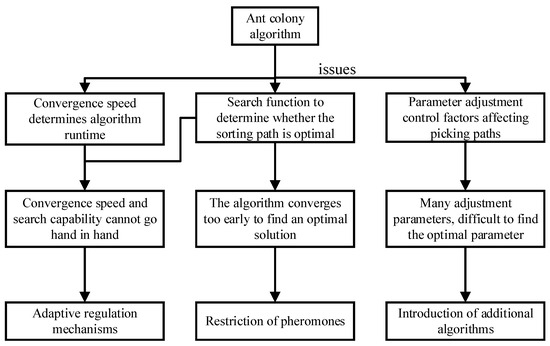
Figure 8.
Optimization analysis of the ant colony algorithm.
2.3.1. Adaptive Regulation Mechanisms
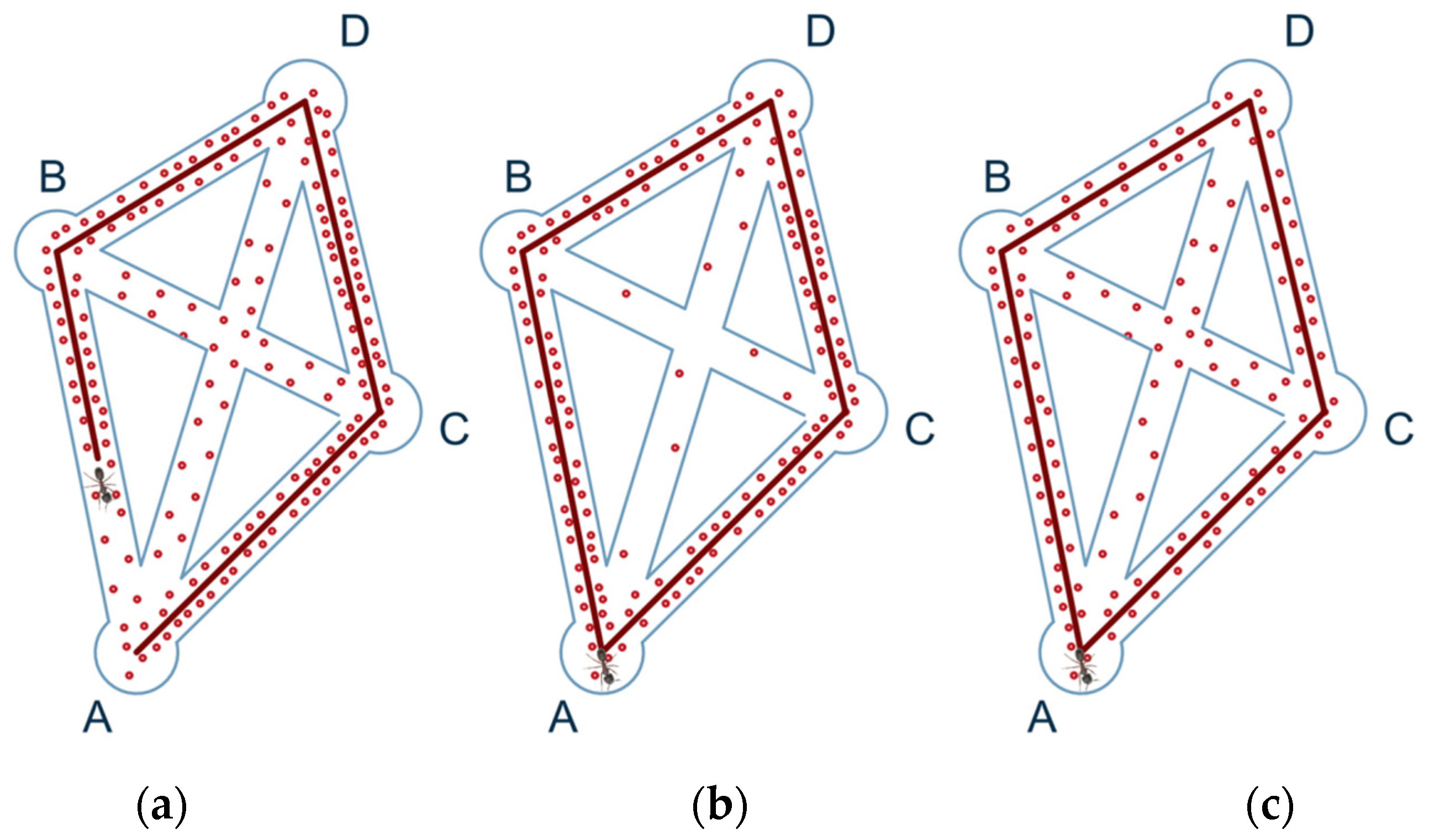
As illustrated in Figure 9, in the basic ant colony algorithm, the pheromone evaporation coefficient is a fixed constant within the range [0,1], and its magnitude is directly related to the global search capability and convergence speed of the ant colony algorithm during the optimization process. To optimize the setting of this parameter, an improved ant colony algorithm adopts an adaptive factor-updating strategy to adjust the value of , catering to the algorithm’s needs at different stages. In the initial phase of the algorithm, is set to a higher value to enhance the global search capability and increase the diversity of safflower harvesting path choices, thereby preventing the algorithm from prematurely converging to local optimum paths. As the algorithm iterates, the value of is gradually decreased to accelerate the convergence speed of the algorithm. This adjustment aims to focus the search on the optimal path more in the later stages, reducing pheromone evaporation to speed up the process of finding the optimal solution and minimizing the waiting time for the robotic arm. This adjustment strategy helps to narrow the search range for harvesting paths in the later stages of the algorithm, preventing the algorithm from diverging in the entire space of the harvesting path search, ensuring the efficient convergence of the algorithm.
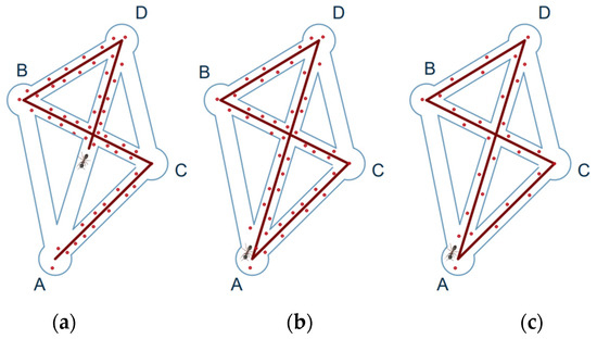
Figure 9.
Adaptive schematic: (a) ants release pheromones; (b) smaller values of; (c) larger values of. Where A, B, C and D are path points that require trajectory planning.
This adaptive adjustment mechanism makes the ant colony algorithm more flexible and efficient in the path planning of safflower-harvesting robotic arms, enabling it to maintain global search capabilities while effectively accelerating the convergence process, thereby enhancing the precision and efficiency of path planning. Therefore, the pheromone evaporation coefficient is dynamically adjusted based on the ratio of the current iteration to the maximum number of iterations, resulting in a decrease in the pheromone evaporation coefficient as the number of iterations increases, as shown in Equation (11):
where is the current iteration number and is the maximum iteration number.
2.3.2. Limiting Pheromones
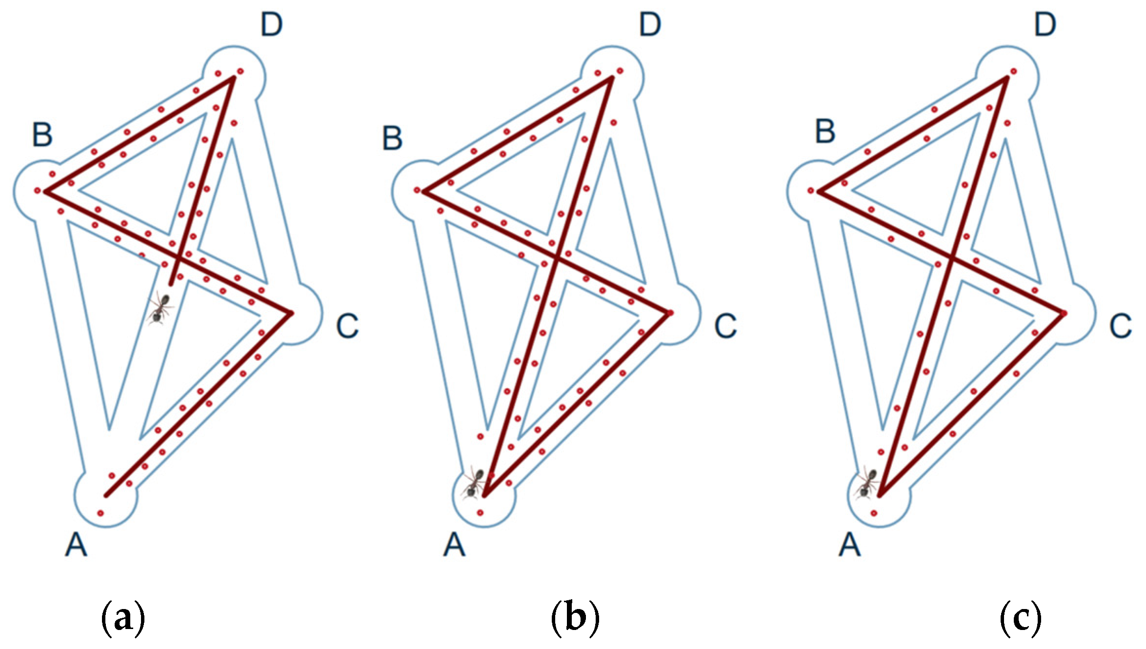
As depicted in Figure 10, in the unimproved ant colony algorithm, ants tend to choose paths where pheromone accumulation is high, leading the algorithm to excessively concentrate on searching within local areas, thereby overlooking some latent optimal paths. This issue is particularly pronounced when certain paths are not searched for an extended period, causing the pheromone on these paths to gradually dissipate due to evaporation, resulting in these paths no longer being searched. Consequently, this can cause the algorithm to stagnate, making it unable to find a superior global solution.
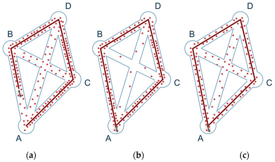
Figure 10.
Schematic diagram of restriction pheromone: (a) ants release pheromone; (b) no limiting pheromone; (c) limiting pheromone. Where A, B, C and D are path points that require trajectory planning.
In this study, we introduce the concept of simplified min-max thinking, specifically, the fixation of the pheromone domain. This approach is designed to prevent the complete evaporation of pheromones on lesser-traveled paths, ensuring that they remain viable options for exploration. By establishing a minimum threshold for pheromone levels, we ensure that all paths have the potential to be explored, thus avoiding the pitfall of the algorithm neglecting potentially optimal but less frequented routes. This strategy helps to maintain a balance between exploration and exploitation, facilitating the algorithm’s ability to escape local optima and enhance its chances of discovering the global optimum.
The initial value of the pheromone is . The method of fixing the pheromone domain ensures that the difference in pheromone levels across various paths is not substantial. This grants ants a broader range of path choices, effectively preventing the algorithm from prematurely converging to a halt and, simultaneously, accelerating the convergence toward the optimal solution.
2.3.3. Parameter Optimization of the Ant Colony Algorithm Based on Genetic Algorithm
This study employs a genetic algorithm to optimize the initial parameters , , , and of the ant colony algorithm, with the aim of enhancing its performance. By integrating the concepts of genetic algorithms into the ant colony system, the approach achieves optimal algorithm performance without the need for manual settings. The specific steps are as follows:
- (1)
- Initializing the population: The genetic algorithm initially generates a certain number of initial populations randomly and encodes them, representing the parameters , , , and with four binary code strings , , , , respectively. These are then combined into a single binary code string. Moreover, based on the findings of previous researchers, it is known that the overall performance of the algorithm is better when is in the range in , and in .
- (2)
- Adaptive function: Genetic algorithms simulate natural genetic mechanisms to tackle optimization problems, where “fitness” serves as a crucial metric for evaluating the extent to which a solution addresses the problem. The fitness function is tailored according to the optimization objective, assessing the effectiveness of each solution. The algorithm selects and propagates optimal solutions based on their fitness, generally without requiring additional information. In this study, the optimal solution is defined as the one that enables the robotic arm to harvest safflower filaments via the shortest possible path. Therefore, the fitness function is formulated as follows:
The fitness function is the reciprocal of the global optimal path length found by the ant colony algorithm, denoted as.
- (3)
- Genetic operators: Consistent with the ant colony algorithm, the selection operation employs the roulette wheel method; the crossover and mutation operations utilize the methods described in Equations (14) and (15), respectively.
Here, is the crossover probability, is the variance probability, is the initial crossover probability, is the initialized variance probability, is the average fitness of the genetic algorithm population, is the genetic algorithm’s population maximal fitness, is the higher fitness value among the two to-be-hybridized individuals, and is the fitness of the mutated individuals.
- (4)
- Algorithm parameter configuration: For the improved ant colony algorithm, the parameter settings are as follows: the number of ants m = 50 and the maximum number of iterations G = 300. For the genetic algorithm, the parameter settings include population size P = 40, the number of iterations set to 200, initial crossover probability = 0.7, and initial mutation probability .
Through the iterations of the above genetic algorithm, the optimal solutions for the uncertain parameters of the ant colony algorithm can be identified. These solutions are then incorporated into the ant colony algorithm to enhance its efficiency. The flowchart of the ant colony genetic algorithm is illustrated in Figure 11.
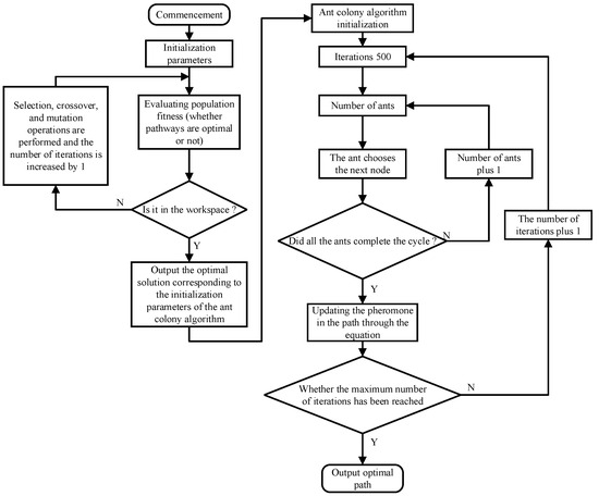
Figure 11.
Flowchart of the ant colony genetic algorithm.
3. Results
3.1. Comparative Analysis of Velocity Profile Models
The improved S-curve speed profile is integrated into the motion control card of the servo motor. Adjustments are made to the supervisory control software, enabling the safflower harvesting robot’s Delta parallel mechanism to complete a work cycle based on the set parameters. This approach also satisfies constraints on speed, acceleration, and jerk, ensuring smooth operation throughout the work process. Two operational conditions, as described in Table 1, are set to compare the S-curve model and the improved S-curve model.

Table 1.
Design value of the task.
Table 2 reveals that, in Condition 1, the improved S-curve speed profile reduced the time from 5.667 s to 5.032 s, achieving an 11.2% time reduction. In Condition 2, the refined S-curve speed profile decreased the time from 3.972 s to 3.088 s, resulting in a 22.3% time reduction. Thus, the enhanced S-curve speed profile significantly reduces the operation time in both Condition 1 and Condition 2.
Table 2.
Optimum working time for reference conditions.
The improved S-curve model can reduce the working time as well as limit the jerk. As indicated in Table 3, it allows for a comparison between the maximum and average jerk at the motor joint. Compared to the S-curve speed model, the improved model can impose restrictions on jerk.
Table 3.
Maximum urgency and average urgency.
A simulation was conducted on the harvesting of safflower filaments in Jimsar County, Xinjiang, to test the viability and efficiency of the proposed improved S-curve speed model within the harvesting cycle. The simulated harvesting covered an area of 1, with mature safflower plants numbering 15 and 30, respectively, for each group, and each set underwent 20 tests. According to the results shown in Table 4, the improved model, when compared to its predecessor, reduces the average working time and decreases the jerk. These results indicate that, while adhering to constraint conditions, the improved S-curve speed model surpasses the original S-curve speed model in terms of jerk and average working time.
Table 4.
Comparison of velocity profile model simulation results.
3.2. Comparative Analysis of Path Planning Algorithms
Based on field photography and statistical analysis of actual safflower spatial distribution samples in Jimsar County, Changji Hui Autonomous Prefecture, Xinjiang, as shown in Figure 12, a safflower harvesting robot simulation system was designed. Simulation experiments were conducted using Matlab2019b software. This study selected the basic ant colony optimization algorithm (ACO) and an ant colony genetic hybrid optimization algorithm for experimental comparative analysis. The experimental environment consisted of a 3.2 GHz AMD Ryzen 7 5800 H processor, 16 GB of memory, and MatlabR2019a as the simulation software.
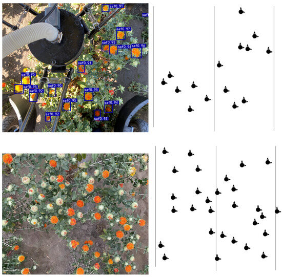
Figure 12.
Field safflower locations.
As shown in Table 5, for 15 and 31 safflower flowers, the genetic algorithm was used to optimize some initial parameters of the improved ant colony algorithm.
Table 5.
Genetic algorithm optimization results safflower flowers.
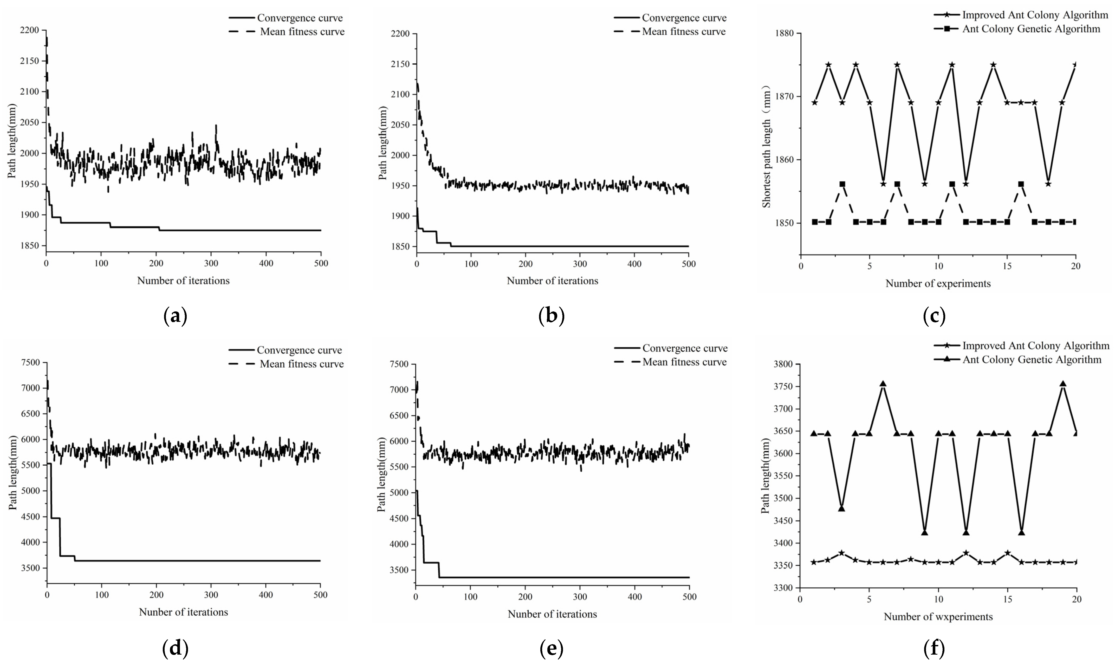
Figure 13 displays the results of 20 independent runs and the convergence curves of the best outcomes for both algorithms when tasked with harvesting 15 and 30 safflower flowers, iterating 200 times. The figure reveals that the ant colony genetic algorithm demonstrates more stable solutions compared to the basic ant colony algorithm and the improved ant colony algorithm, capable of finding better solutions. In all 20 independent runs, the ant colony genetic algorithm consistently converged to the optimal solution more effectively than the other algorithms. These results indicate that the ant colony genetic algorithm successfully addresses issues of premature convergence and overly rapid convergence speeds. Moreover, in all 20 independent runs, the ant colony genetic algorithm can plan shorter continuous harvesting paths, making continuous harvesting more efficient. For a more intuitive understanding of the harvesting paths, the three-dimensional coordinates and harvesting paths of 15 safflower flowers were visualized, as shown in Figure 14.

Figure 13.
Algorithm optimization results. (a) Iteration curve of the improved ant colony algorithm based on 15 safflower flowers; (b) Iteration curve of the ant colony genetic algorithm based on 15 safflower flowers; (c) Lengths of 20 optimized paths based on 15 safflower flowers; (d) Iteration curve of the improved ant colony algorithm based on 30 safflower flowers; (e) Iteration curve of the ant colony genetic algorithm based on 30 safflower flowers; (f) Lengths of 20 optimized paths based on 30 safflower flowers.

Figure 14.
Ant colony genetic algorithm picking trajectory map.
3.3. Field Experiment Validation
Field experiments were carried out to examine the distribution of two types of safflower filaments by conducting 20 harvesting trials, as depicted in Figure 15. Table 6 indicates that, under the same harvesting cycle, the safflower harvesting robot employing the ant colony genetic algorithm required from 6.8% to 8.3% less time to complete a work cycle compared to the basic ant colony algorithm, and it was 32.8% to 35.2% faster than sequential random harvesting. Consequently, the experiments demonstrate that the safflower-harvesting robot can efficiently complete a harvesting cycle in field conditions, significantly enhancing the operational efficiency of the safflower-harvesting robotic arm.
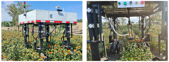
Figure 15.
Safflower-picking robot field experiment.
Table 6.
Genetic algorithm optimization results safflower harvesting.
4. Discussion
This study introduced a trajectory planning scheme aimed at enhancing the efficiency of safflower filament harvesting. The model, designed based on the growth patterns in safflower fields, generates smoother and more continuous curves for velocity, acceleration, and jerk, thereby significantly improving the motion stability and positioning accuracy of parallel robotic arms. Additionally, by simplifying the continuous safflower-harvesting path problem into a traveling salesman problem (TSP) without considering obstacle avoidance, an ant colony genetic algorithm was proposed. The simulation results indicate that, compared to the basic ant colony algorithm, the path length with the ant colony genetic algorithm is reduced by 1.33% to 7.85%, and it also shows superior convergence stability. Moreover, field trials demonstrated that, under the premise of maintaining S-curve velocity, the ant colony genetic algorithm reduces harvesting time by 28.25% to 35.18% compared to random harvesting and by 6.34% to 6.81% compared to the basic ant colony algorithm. This significantly enhances the harvesting efficiency of the safflower-harvesting robotic arm.
Author Contributions
Conceptualization, Z.Q. and H.G.; methodology, Z.Q.; software, Z.Q.; validation, Z.Q., G.G. and T.W.; formal analysis, H.C.; investigation, X.W.; resources, H.G.; data curation, Z.Q.; writing—original draft preparation, Z.Q.; writing—review and editing, Z.Q. and H.G.; supervision, G.G.; project administration, H.G.; funding acquisition, H.G. All authors have read and agreed to the published version of the manuscript.
Funding
This study was supported by the Natural Science Foundation of Xinjiang Uygur Autonomous Region (No. 2022D01A177) and the Xinjiang Agricultural University Graduate Student Research and Innovation Project (No. XJAUGRI2023014).
Institutional Review Board Statement
Not applicable.
Data Availability Statement
The data presented in this study are available upon request from the corresponding author. The data are not publicly available as the device is in the research and development stage; it needs to be further studied and improved.
Conflicts of Interest
The funders had no role in the design of the study; in the collection, analyses, or interpretation of data; in the writing of the manuscript; or in the decision to publish the results.
References
- Zhou, Y.H.; Guo, J.F.; Ma, X.L.; Fan, X.Q.; Chen, Y.; Lin, M. Research on Current Situation and Development Countermeasures of Xinjiang Safflower Production. J. Anhui Agric. Sci. 2021, 49, 199–201, 217. [Google Scholar]
- Yang, H. Research Status of Mechanized Harvesting of Safflower Silk in Xinjiang. J. Agric. Mech. Res. 2020, 5, 34–37. [Google Scholar]
- Hatim, M.; Majidian, M.; Tahmasebi, M.; Nabavi-Pelesaraei, A. Life cycle assessment, life cycle cost, and exergoeconomic analysis of different tillage systems in safflower production by micronutrients. Soil Tillage Res. 2023, 233, 105795. [Google Scholar] [CrossRef]
- Mani, V.; Lee, S.K.; Yeo, Y.; Hahn, B.S. A Metabolic Perspective and Opportunities in Pharmacologically Important Safflower. Metabolites 2020, 10, 253. [Google Scholar] [CrossRef]
- Zhang, H.; Ge, Y.; Sun, C.; Zeng, H.; Liu, N. Picking path planning method of dual rollers type safflower picking robot based on improved ant colony algorithm. Processes 2022, 10, 1213. [Google Scholar] [CrossRef]
- Gao, G.; Guo, H.; Zhou, W.; Luo, D.; Zhang, J. Design of a control system for a safflower picking robot and research on multisensor fusion positioning. Eng. Agrícola 2023, 43, e20210238. [Google Scholar] [CrossRef]
- Cao, R.Y.; Zhang, Z.Q.; Li, S.C.; Zhang, M.; Li, H.; Li, Z.M. Multi-machine Cooperation Global Path Planning Based on A-star Algorithm and Bezier Curve. Trans. Chin. Soc. Agric. Mach. 2021, 52, 548–554. [Google Scholar]
- Li, G.; Wang, Y. Time-optimal trajrctory planning of robots based on B-spline and improved grnrtic algorithm. Comput. Appl. Softw. 2020, 37, 215–223+279. [Google Scholar]
- Liu, C.; Cao, G.H.; Qu, Y.Y.; Cheng, Y.M. An improved PSO algorithm for time-optimal trajectory planning of Delta robot in intelligent packaging. Int. J. Adv. Manuf. Technol. 2020, 107, 1091–1099. [Google Scholar] [CrossRef]
- Wu, M.; Mei, J.; Zhao, Y.; Niu, W. Vibration reduction of delta robot based on trajectory planning. Mech. Mach. Theory 2020, 153, 104004. [Google Scholar] [CrossRef]
- Fang, S.; Cao, J.; Zhang, Z.; Zhang, Q.; Cheng, W. Study on high-speed and smooth transfer of robot motion trajectory based on modified s-shaped acceleration/deceleration algorithm. IEEE Access 2020, 8, 199747–199758. [Google Scholar] [CrossRef]
- Lu, S.; Ding, B.; Li, Y. Minimum-jerk trajectory planning pertaining to a translational 3-degree-of-freedom parallel manipulator through piecewise quintic polynomials interpolation. Adv. Mech. Eng. 2020, 12, 1687814020913667. [Google Scholar] [CrossRef]
- Qi, M.; Dou, L.; Xin, B. 3D Smooth Trajectory Planning for UAVs under Navigation Relayed by Multiple Stations Using Bézier Curves. Electronics 2023, 12, 2358. [Google Scholar] [CrossRef]
- Wang, R.; Jiang, T.; Bai, G.; Wang, Y.; Wang, S.; Tan, M. Stepwise Cooperative Trajectory Planning for Multiple BUVs Based on Temporal–Spatial Bezier Curves. IEEE Trans. Instrum. Meas. 2023, 72, 1–14. [Google Scholar] [CrossRef]
- Ren, L.; Wang, N.; Cao, W.; Li, J.; Ye, X. Trajectory planning and motion control of full-row seedling pick-up arm. Int. J. Agric. Biol. Eng. 2020, 13, 41–51. [Google Scholar] [CrossRef]
- Lai, R.; Wu, Z.; Liu, X.; Zeng, N. Fusion Algorithm of the Improved A* Algorithm and Segmented Bézier Curves for the Path Planning of Mobile Robots. Sustainability 2023, 15, 2483. [Google Scholar] [CrossRef]
- Yao, X.; Li, Z.; Cheng, X. Research on Robot Path Planning Based on Improved Ant Colony Algorithm. Comput. Simul. 2021, 38, 379–383. [Google Scholar]
- Ren, T.; Luo, T.; Li, X.; Xiang, S.; Xiao, H.L.; Xing, L.N. Knowledge based ant colony algorithm for cold chain logistics distribution path optimization. Control Decis. 2022, 37, 545–554. [Google Scholar]
- Hu, Z.; Luo, L.; Lv, Y.; Luo, Y. Path planning of mobile robot based on potential field oriented logarithmic ant colony algorithm. J. Chongqing Univ. Posts Telecommun. (Nat. Sci. Ed.) 2021, 33, 498–506. [Google Scholar]
- Zhao, W.; Zhou, D. An Improved Path Planning Algorithm Based on the Fusion of A* and Third-order Bessel Curves. J. Anhui Univ. Technol. (Nat. Sci.) 2023, 40, 333–338. [Google Scholar]
- de Winkel, K.N.; Irmak, T.; Happee, R.; Shyrokau, B. Standards for passenger comfort in automated vehicles: Acceleration and jerk. Appl. Ergon. 2023, 106, 103881. [Google Scholar] [CrossRef] [PubMed]
- Wu, L.; Huang, X.; Cui, J.; Liu, C.; Xiao, W. Modified adaptive ant colony optimization algorithm and its application for solving path planning of mobile robot. Expert Syst. Appl. 2023, 215, 119410. [Google Scholar] [CrossRef]
- Li, S.; Zhang, M.; Wang, N.; Cao, R.; Zhang, Z.; Ji, Y.; Li, H.; Wang, H. Intelligent scheduling method for multi-machine cooperative operation based on NSGA-III and improved ant colony algorithm. Comput. Electron. Agric. 2023, 204, 107532. [Google Scholar] [CrossRef]
- Comert, S.E.; Yazgan, H.R. A new approach based on hybrid ant colony optimization-artificial bee colony algorithm for multi-objective electric vehicle routing problems. Eng. Appl. Artif. Intell. 2023, 123, 106375. [Google Scholar] [CrossRef]


Disclaimer/Publisher’s Note: The statements, opinions and data contained in all publications are solely those of the individual author(s) and contributor(s) and not of MDPI and/or the editor(s). MDPI and/or the editor(s) disclaim responsibility for any injury to people or property resulting from any ideas, methods, instructions or products referred to in the content. |
© 2024 by the authors. Licensee MDPI, Basel, Switzerland. This article is an open access article distributed under the terms and conditions of the Creative Commons Attribution (CC BY) license (https://creativecommons.org/licenses/by/4.0/).