Model and Parameter Adaptive MPC Path Tracking Control Study of Rear-Wheel-Steering Agricultural Machinery

Abstract

To further enhance the precision and the adaptability of path tracking control, and considering that most of the research is focused on front-wheel steering, an adaptive parametric model predictive control (MPC) was proposed for rear-wheel-steering agricultural machinery. Firstly, the kinematic and dynamic models of rear-wheel-steering agricultural machinery were established. Secondly, the influence laws of curvature and velocity on the prediction horizon N_p, control horizon N_c, and preview value N_pre were obtained by simulating and analyzing the factors influencing the MPC tracking effect. The results revealed that raising N_pre can improve curve tracking performance. N_p was correlated negatively with the curvature change, whereas N_c and N_pre were positively connected. N_p, N_c, and N_pre were correlated positively with the velocity change. Then, the parameters for self-adaptation of N_p, N_c, and N_pre were accomplished via fuzzy control (FC), and particle swarm optimization (PSO) was utilized to optimize the three parameters to determine the optimal parameter combination. Finally, simulation and comparative analysis were conducted to assess the tracking effects of the manual tuning MPC, the FC_MPC, and the PSO_MPC under U-shaped and complex curve paths. The results indicated that there was no significant difference and all three methods achieved better tracking effects under no disturbance, with the mean absolute value of lateral error ≤0.18 cm, standard deviation ≤0.37 cm, maximum deviation of U-shaped path <2.38 cm, and maximum deviation of complex curve path <3.15 cm. The mean absolute value of heading error was ≤0.0096 rad, the standard deviation was ≤0.0091 rad, and the maximum deviation was <0.0325 rad, indicating that manual tuning can find optimal parameters, but with high uncertainty and low efficiency. However, FC_MPC and PSO_MPC have better adaptability and tracking performance compared to the manual tuning MPC with fixed horizons under variable-speed disturbance and are more able to meet the actual needs of agricultural machinery operations.

1. Introduction

The autonomous driving of agricultural machinery is critical to accomplish the “replacement of manual labor with machines” and answer the question of “who will farm in the future” [1]. Path tracking control is at the heart of autonomous driving technology, which is widely used in farming, planting, management, harvesting, transportation, and other aspects of agricultural production to improve work quality and efficiency and to reduce the waste of agricultural production materials [2]. Typical path tracking control methods include geometric model-based PP [3] and Stanley [4], etc., kinematic and dynamic model-based PID [5], LQR [6], SMC [7], and MPC [8], etc., as well as model-free based fuzzy control [9], reinforcement learning [10], and neural networks [11], etc.

MPC is the most widely used control method in practice other than PID, according to a survey by the International Federation of Automatic Control [12]. MPC can handle constraint problems in real time and has low requirements for the accuracy of the control model. It is suitable for both linear and nonlinear systems, but tracking accuracy is difficult to guarantee at high speeds [13,14]. Therefore, it has unique advantages for agricultural machinery path tracking with relatively low operation speed, complex ground conditions, and difficulty in establishing accurate models. Xue et al. constructed a kind of MPC controller utilizing a linear time-varying model for orchard tractors, with average lateral errors of 7 cm and 13 cm for curve tracking at 2.5 m/s and 5 m/s, respectively [15]. He et al. built a kind of MPC controller for rice transplanters upon a kinematic model with attitude correction, and field experiments indicated that the average absolute error was 3.3 cm under a three-line linear path [16].

The initial parameter settings and weights of the components in the optimization objective have a significant impact on the computational results and directly affect the final tracking effect since MPC is essentially an optimization solution method. Neural networks, fuzzy control, and intelligent search algorithms are commonly used parameter adaptation methods. Different methods have their benefits as well as limitations. The selection process is primarily oriented to the actual demand (e.g., control accuracy, stability, adaptability, etc.), and the control results (e.g., tracking error) are measured as the indexes. Simultaneously, the computational capability of the implementation hardware is also taken into account. Zhou et al. applied the genetic algorithm to calculate the optimal time-domain parameters for articulated steering tractors, with an average lateral error of 2.1 cm under U-shaped path tracking, while the traditional MPC was 7.53 cm [17]. Wang et al. utilized the fuzzy principle to achieve the adaptive error weight coefficients of MPC, and the simulation results demonstrated the superiority of the upgraded MPC tracking effect over the PP controller [18]. Shi et al. used PSO-BPNN to improve MPC in the prediction and control horizon under different road adhesion coefficients [19]. Guan et al. dynamically adjusted the MPC’s feedforward factor and lateral error weight based on BPNN. The maximum lateral error was 5.13 cm under double-lane path tracking and 9.23 cm for conventional MPC when the speed was 28 km/h [20]. Liang et al. used RBF neural networks to adaptively compensate for errors caused by changes in the curvature of complex paths at high speed, with a maximum error of 0.285 m [21]. Lin et al. adopted fuzzy control to optimize the prediction and control horizon online with v_x and v_y as inputs and the horizon factor as output [22]. Dai et al. proposed a kind of MPC with adaptive preview characteristics, and the maximum lateral error was 0.04 m at 10 m/s under double-lane path tracking by the simulation outcomes [23]. Choi et al. updated the sample time in the subsequent iteration based on the control inputs in each iteration of MPC and simulated the superiority of this method [24]. Liu et al. proposed a two-layer MPC with curvature adaption, which has strong adaptability at high speeds [25]. As can be seen from the above, traditional MPC with fixed parameters has poor adaptability to working conditions. The adaptation of key parameters such as time domain and error weights has become a research hotspot, but there is still significant space for improvement in terms of control precision and applicability, making this a crucial area for further study.

The steering methods of wheeled agricultural machinery mainly include front-wheel steering (such as tractors, transplanters, etc.), rear-wheel steering (such as grain harvesters, residual film recyclers, etc.), and four-wheel steering (such as high-clearance sprayers [26], etc.). Current research on agricultural vehicle models mainly focuses on front-wheel steering [27], with less research on the kinematic and dynamic models of rear-wheel-steering agricultural machinery, blurring or ignoring the difference between them, and equating them for control research.

To further improve the precision of path tracking and the adaptability of the control system to various operating conditions, and given that most research focuses on front-wheel steering, this study accomplished the following: (1) established the kinematic model and dynamic model of rear-wheel-steering agricultural machinery; (2) simulated and analyzed the key factors affecting the tracking effect, and discovered the interaction laws; (3) achieved the self-adaptation of the key parameters of MPC utilizing the fuzzy control and PSO, and then designed the path-tracking controller to compare and analyze the parameter adaptive MPC’s tracking effect with that of the traditional manual tuning MPC, proving the superiority of the designed controller.

2. Materials and Methods

2.1. Vehicle Model of Rear-Wheel-Steering Agricultural Machinery

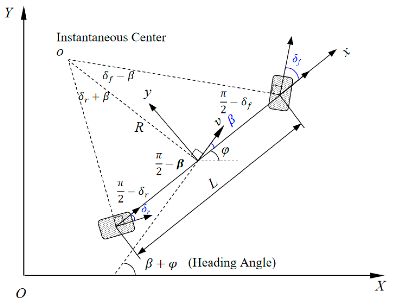
2.1.1. Kinematic Model

Figure 1 represents the kinematic model of agricultural machinery schematically.

The vehicle’s kinematic equation is as follows, according to the geometric relationship of the steering:

$$\left\{\begin{array}{l}\dot{x}=v\cos (\beta +\varphi )\hfill \\ \dot{y}=v\sin (\beta +\varphi )\hfill \\ \dot{\varphi }=\frac{v(\tan {\delta }_f+\tan {\delta }_r)\cos \beta }{L}\hfill \end{array}\right.$$

(1)

Under low-speed conditions (the operation speed of the agricultural machinery is usually <3 m/s), assuming that the vehicle has no side-slip, i.e., v_y = 0, then $\beta =\arctan \frac{v_y}{v_x}=0$. In agricultural machinery with rear-wheel steering, the front-wheel steering angle δ_f = 0; therefore, its kinematic equation is as follows:

$$\left\{\begin{array}{l}\dot{x}=v\cos \varphi \hfill \\ \dot{y}=v\sin \varphi \hfill \\ \dot{\varphi }=\frac{v\tan {\delta }_r}{L}\hfill \end{array}\right.$$

(2)

Select $\chi ={[x,y,\varphi ]}^T$ as the state variables and $u={[v,\delta ]}^T$ as the control variables. The error state equation is obtained by performing a Taylor series expansion at the reference point, neglecting high-order terms, and calculating the Jacobian matrix.

$$\dot{\tilde{\chi }}=\left[\begin{array}{ccc}0& 0& -v_r\sin {\varphi }_r\\ 0& 0& v_r\cos {\varphi }_r\\ 0& 0& 0\end{array}\right]\left[\begin{array}{c}x-x_r\\ y-y_r\\ \varphi -{\varphi }_r\end{array}\right]+\left[\begin{array}{cc}\begin{array}{c}\cos {\varphi }_r\\ \begin{array}{c}\sin {\varphi }_r\\ \frac{\tan {\delta }_r}{L}\end{array}\end{array}& \begin{array}{c}0\\ \begin{array}{c}0\\ \frac{v_r}{L{\cos }^2{\delta }_r}\end{array}\end{array}\end{array}\right]\left[\begin{array}{c}v-v_r\\ \delta -{\delta }_r\end{array}\right]=a\tilde{\chi }+b\tilde{u}$$

(3)

The error state equation is discretized using the forward Euler method, to facilitate the design of the MPC controller. The discrete error model of the system is as follows:

$$\tilde{\chi }\left(k+1\right)=\tilde{a}\tilde{\chi }\left(k\right)+\tilde{b}\tilde{u}\left(k\right)$$

(4)

where $\tilde{a}=\left[\begin{array}{ccc}1& 0& -T{v}_r\sin {\varphi }_r\\ 0& 1& T{v}_r\cos {\varphi }_r\\ 0& 0& 0\end{array}\right]$, $\tilde{b}=\left[\begin{array}{cc}\begin{array}{c}T\cos {\varphi }_r\\ \begin{array}{c}T\sin {\varphi }_r\\ \frac{T\tan {\delta }_r}{L}\end{array}\end{array}& \begin{array}{c}0\\ \begin{array}{c}0\\ \frac{T{v}_r}{L{\cos }^2{\delta }_r}\end{array}\end{array}\end{array}\right]$, and T is the sampling time.

2.1.2. Dynamic Model

The dynamic model of rear-wheel-steering agricultural machinery is schematically depicted in Figure 2, taking into account the two degrees of freedom in the lateral and yaw directions.

The two-degree-of-freedom (2DoF) dynamic equation for rear-wheel-steering agricultural machinery is derived as follows:

$$m(\ddot{y}+v_x\dot{\varphi })=2C_{cf}(-\frac{v_y+l_f\dot{\varphi }}{v_x})+2C_{cr}({\delta }_r-\frac{v_y-l_r\dot{\varphi }}{v_x})$$

(5)

$$I_z\ddot{\varphi }=2l_f{C}_{cf}(-\frac{v_y+l_f\dot{\varphi }}{v_x})-2l_r{C}_{cr}({\delta }_r-\frac{v_y-l_r\dot{\varphi }}{v_x})$$

(6)

where m is the mass of the vehicle; I_z is the moment of inertia around the z-axis of the vehicle; C_cf and C_cr are the lateral stiffness of the front and rear wheels respectively.

Choose $\chi ={\left[y,\dot{y},\varphi ,\dot{\varphi }\right]}^T$ as the state variables (i.e., lateral position, lateral position change rate, yaw angle, and yaw angle change rate). Set the rear-wheel angle as the control variable, i.e., $u=\left[{\delta }_r\right]$. The state space equation is as follows:

$$\frac{d}{dt}\left[\begin{array}{c}y\\ \dot{y}\\ \varphi \\ \dot{\varphi }\end{array}\right]=\left[\begin{array}{cccc}0& 1& 0& 0\\ 0& -\frac{2C_{cf}+2C_{cr}}{m{v}_x}& 0& -\frac{2C_{cf}{l}_f-2C_{cr}{l}_r}{m{v}_x}-v_x\\ 0& 0& 0& 1\\ 0& \frac{2l_r{C}_{cr}-2l_f{C}_{cf}}{I_z{v}_x}& 0& -\frac{2l_r^2{C}_{cr}+2l_f^2{C}_{cf}}{I_z{v}_x}\end{array}\right]\left[\begin{array}{c}y\\ \dot{y}\\ \varphi \\ \dot{\varphi }\end{array}\right]+\left[\begin{array}{c}0\\ \frac{2C_{cr}}{m}\\ 0\\ -\frac{2l_r{C}_{cr}}{I_z}\end{array}\right]{\delta }_r$$

(7)

Rewrite Equation (7) as follows:

$$\dot{\chi }=a\chi +bu$$

(8)

The response of the vehicle’s lateral displacement, yaw angle, lateral velocity, and yaw angular rate can be analyzed under a given steering angle input according to the system state equation. However, as the goal of tracking control is to minimize tracking deviation, the state equation ought to be able to analyze the vehicle’s tracking deviation under a given angle. Therefore, it is necessary to transform Equation (8) into the tracking error state space equation.

Set $\tilde{\chi }={\left[\tilde{y},\dot{\tilde{y}},\tilde{\varphi },\dot{\tilde{\varphi }}\right]}^T$ as the state variables (i.e., lateral position error, lateral position error change rate, yaw angle error, and yaw angle error change rate). The tracking error state space equation of the dynamic model for rear-wheel-steering agricultural machinery is as follows:

$$\frac{d}{dt}\left[\begin{array}{c}\tilde{y}\\ \dot{\tilde{y}}\\ \tilde{\varphi }\\ \dot{\tilde{\varphi }}\end{array}\right]=\left[\begin{array}{cccc}0& 1& 0& 0\\ 0& -\frac{2C_{cf}+2C_{cr}}{m{v}_x}& \frac{2C_{cf}+2C_{cr}}{m}& -\frac{2C_{cf}{l}_f-2C_{cr}{l}_r}{m{v}_x}\\ 0& 0& 0& 1\\ 0& \frac{2l_r{C}_{cr}-2l_f{C}_{cf}}{I_z{v}_x}& -\frac{2l_r{C}_{cr}-2l_f{C}_{cf}}{I_z}& -\frac{2l_r^2{C}_{cr}+2l_f^2{C}_{cf}}{I_z{v}_x}\end{array}\right]\left[\begin{array}{c}\tilde{y}\\ \dot{\tilde{y}}\\ \tilde{\varphi }\\ \dot{\tilde{\varphi }}\end{array}\right]+\left[\begin{array}{c}0\\ \frac{2C_{cr}}{m}\\ 0\\ -\frac{2l_r{C}_{cr}}{I_z}\end{array}\right]{\delta }_r$$

(9)

Rewrite Equation (9) as follows:

$$\dot{\tilde{\chi }}=\tilde{a}\tilde{\chi }+\tilde{b}u$$

(10)

According to Equations (8) and (10), path tracking can be accomplished by utilizing MPC to obtain the appropriate amount of control at the lowest possible cost, hence lowering the tracking error.

The kinematic model is simple and practical, suitable for situations with low speeds and infrequent curvature changes. Nevertheless, it disregards the force interacting between wheels and ground, which can lead to side-slip at high speeds. The dynamic model considers the ground–wheel interactions and more vehicle physics, but it is more complex and requires balancing computational accuracy and real-time performance due to its difficult-to-access modeling parameters. This paper takes the kinematic model as the control model since agricultural machines have low speeds and complex ground conditions

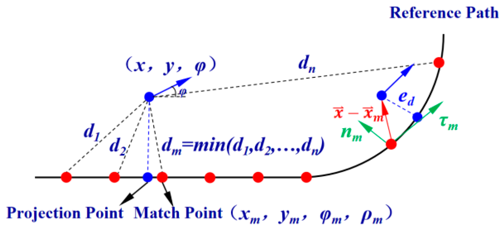
2.2. Model Predictive Control

To obtain the optimal control sequence at the current moment, the MPC controller performs an optimization solution based on the prediction model, objective function, and constraint conditions. The principle can be summarized as predictive modeling, rolling optimization, and feedback correction.

2.2.1. Objective Function

To achieve a more stable path-tracking effect, the control quantity increments are constrained and new state variables are constructed.

$$\xi (k)={\left[\begin{array}{cc}\tilde{\chi }(k)& \tilde{u}(k-1)\end{array}\right]}^T$$

(11)

Substitute Equation (11) into the state space equation to obtain a new state space expression and output equation:

$$\left\{\begin{array}{l}\xi (k+1)=A\xi (k)+B\mathsf{\Delta }\tilde{u}(k)\hfill \\ \eta (k)=C\xi (k)\hfill \end{array}\right.$$

(12)

where $A=\left[\begin{array}{cc}\tilde{a}& \tilde{b}\\ O_{N_u\times N_x}& I_{N_u}\end{array}\right], B=\left[\begin{array}{c}\tilde{b}\\ I_{N_u}\end{array}\right], C=\left[\begin{array}{cc}{I}_{N_x}& O_{N_u\times N_x}\end{array}\right], \mathsf{\Delta }\tilde{u}(k)=\tilde{u}(k)-\tilde{u}(k-1)$

N_x and N_u are the state and control quantity dimensions, respectively; I and O are the identity and zero matrix, respectively; and η is the new output variable.

Then the output equation can be expressed as follows:

$$Y=\Psi \xi (k)+\Theta \mathsf{\Delta }U$$

(13)

where $Y={\left[\begin{array}{cccc}\eta (k+1)& \eta (k+2)& \cdots & \eta (k+N_p)\end{array}\right]}^T, \Psi ={\left[\begin{array}{cccc}CA& C{A}^2& \cdots & C{A}^{N_p}\end{array}\right]}^T,$

$$\begin{gathered} \Theta =\left[\begin{array}{cccc}CB& 0& \cdots & 0\\ CAB& CB& \cdots & 0\\ ⋮& ⋮& \ddots & ⋮\\ C{A}^{N_c-1}B& C{A}^{N_c-2}B& \cdots & C{A}^{0}B\\ ⋮& ⋮& \ddots & ⋮\\ C{A}^{N_p-1}B& C{A}^{N_p-2}B& \cdots & C{A}^{N_p-N_c}B\end{array}\right], \mathsf{\Delta }U={\left[\begin{array}{cccc}\mathsf{\Delta }\tilde{u}(k)& \mathsf{\Delta }\tilde{u}(k+1)& \\ \cdots & \mathsf{\Delta }\tilde{u}(k+N_c-1)\end{array}\right]}^T \end{gathered}$$

N_p and N_c (N_p > N_c) are the prediction and control horizon, respectively.

Thus, the output in N_p can be predicted if the present $\xi (k)$ and $\mathsf{\Delta }U$ in the control horizon are known.

It is expected to achieve the reference value of the state variable as quickly as possible with the minimum control quantity while ensuring stationarity in path tracking control. Therefore, the optimization objective function can be expressed as follows:

$$\begin{array}{l}J={\tilde{Y}}^T{Q}_Q\tilde{Y}+\mathsf{\Delta }{U}^T{R}_R\mathsf{\Delta }U\\ ={(Y-Y_r)}^T{Q}_Q(Y-Y_r)+\mathsf{\Delta }{U}^T{R}_R\mathsf{\Delta }U\end{array}$$

(14)

where $Q_Q=I_{N_p}\otimes Q_{N_x\times N_p},R_R=I_{N_p}\otimes R_{N_u\times N_c}$, Q and R are the state and quantity weight, respectively; and Y_r is the system output reference value, $Y_r={\left[\begin{array}{cccc}0& 0& \cdots & 0\end{array}\right]}^T$.

To facilitate the computational solution, the objective function is converted by the rounding method into the standard quadratic form:

$$\underset{\Delta U}{\min }J=\frac{1}{2}\mathsf{\Delta }{U}^{T}H\mathsf{\Delta }U+g^T\Delta U$$

(15)

where $H={\Theta }^T{Q}_Q\Theta +R_R, g=E^T{Q}_Q\Theta , E=\Psi \xi (k)$. A relaxation factor $\epsilon$ is included to prevent the equation from having no solution, and the augmented vectors of H and g are as follows: $H=\left[\begin{array}{cc}{\Theta }^T{Q}_Q\Theta +R_R& 0\\ 0& \epsilon \end{array}\right], g=\left[\begin{array}{c}{E}^T{Q}_Q\Theta \\ \epsilon \end{array}\right]$.

2.2.2. Constraint Condition

The control quantities at each moment in the control horizon satisfy the following equations:

$$\begin{array}{c}U=\left[\begin{array}{c}u(k)\\ u(k+1)\\ ⋮\\ u(k+N_c-1)\end{array}\right]=\left[\begin{array}{c}u(k-1)\\ u(k-1)\\ ⋮\\ u(k-1)\end{array}\right]+\left[\begin{array}{cccc}{I}_2& 0& \cdots & 0\\ I_2& I_2& \cdots & 0\\ ⋮& ⋮& \ddots & ⋮\\ I_2& I_2& \cdots & I_2\end{array}\right]\left[\begin{array}{c}\Delta u(k)\\ \Delta u(k+1)\\ ⋮\\ \Delta u(k+N_c-1)\end{array}\right]=U_t+A_I\Delta U_t\\ U_{\min }={\left[\begin{array}{cccc}{u}_{\min }& u_{\min }& \cdots & u_{\min }\end{array}\right]}^T\le U\le {\left[\begin{array}{cccc}{u}_{\max }& u_{\max }& \cdots & u_{\max }\end{array}\right]}^T=U_{\max }\\ \Delta U_{\min }={\left[\begin{array}{cccc}\Delta u_{\min }& \Delta u_{\min }& \cdots & \Delta u_{\min }\end{array}\right]}^T\le \Delta U\le {\left[\begin{array}{cccc}\Delta u_{\max }& \Delta u_{\max }& \cdots & \Delta u_{\max }\end{array}\right]}^T=\Delta U_{\max }\end{array}$$

(16)

Rewrite Equation (16) as follows:

$$\left\{\begin{array}{c}{A}_I\mathsf{\Delta }{U}_t\le U_{\max }-U_t\\ -A_I\mathsf{\Delta }{U}_t\le -U_{\min }+U_t\\ \mathsf{\Delta }{U}_{\min }\le \mathsf{\Delta }U\le \mathsf{\Delta }{U}_{\max }\end{array}\right.$$

(17)

For the standard quadratic programming problem, the MATLAB (2021b) QP solver “quadprog” is used for solving. Finally, a sequence of control increments in N_c is derived:

$$\mathsf{\Delta }{U}_k^{\ast }={\left[\begin{array}{cccc}\mathsf{\Delta }{\tilde{u}}_k^{\ast }& \mathsf{\Delta }{\tilde{u}}_{k+1}^{\ast }& \cdots & \mathsf{\Delta }{\tilde{u}}_{k+N_c-1}^{\ast }\end{array}\right]}^T$$

(18)

Apply the first element of the control sequence to the controlled object, and the system continues to execute it until the next moment. Repeat the above operation in the next cycle.

$$u(k)=u(k-1)+\mathsf{\Delta }{\tilde{u}}_k^{\ast }$$

(19)

2.3. Analysis of Factors Influencing MPC Tracking Performance

It is vital to explore the impacts of the initial control parameters and the vehicle’s original parameters on MPC since MPC is an optimization method, and the setting of its initial parameters has a significant impact on the solution results.

Typically, agricultural machinery operates at a speed of less than 3 m/s. The operating speed in the simulation below was set to 3 m/s, except for the speed impact analysis.

Table 1. Control parameter settings.

Parameters	Values
Prediction horizon Np	Dynamic adjustment
Control horizon Nc
Preview value Npre
State quantity weight Q	100
Control increment weight R	1
Relaxation factor $\epsilon$	10
Control minimum ${\tilde{u}}_{\min }$/rad	${[\begin{array}{cc}-0.2& -0.54\end{array}]}^T$
Control maximum ${\tilde{u}}_{\max }$/rad	${[\begin{array}{cc}0.2& 0.54\end{array}]}^T$
Control increment minimum $\mathsf{\Delta }{\tilde{u}}_{\min }$/rad	${[\begin{array}{cc}-0.05& -0.2\end{array}]}^T$
Control increment maximum $\mathsf{\Delta }{\tilde{u}}_{m\mathrm{ax}}$/rad	${[\begin{array}{cc}0.05& 0.2\end{array}]}^T$
Sampling period T/s	0.1

displays the other MPC control parameter settings, excluding the dynamically modified parameters. A MATLAB-based simulation environment was built for agricultural machinery path tracking control and the factors affecting tracking performance were analyzed.

2.3.1. Impact of Wheelbase on Tracking Effect

The wheelbase L is the only inherent physical property of the vehicle taken into account in the kinematic model. In agricultural machinery, the wheelbase is typically customized to a non-standard value according to the needs of specific applications. The following simulation analyzed the effect of a typical wheelbase on the effectiveness of path tracking, with settings N_p = 10 and N_c = 2.

As shown in

Table 2. Parameters of tracking effect at different wheelbases under straight paths.

Wheelbase /m	Online Time /s	Online Distance /m	Absolute Value of Lateral Error
			Mean Value /m	Standard Deviation/m	Maximum Error/m
L = 1.5	3	8.7	0.0005	0.0027	0.0216
L = 2.9	3.6	10.7	0.0007	0.0029	0.0232
L = 3.7	3.9	11.7	0.0007	0.0031	0.0243

and Figure 3, with the same initial position and heading angle, the online distances are 8.7 m, 10.7 m, and 11.7 m, and the online times are 3 s, 3.6 s, and 3.9 s, respectively, when the wheelbases are 1.5 m, 2.9 m, and 3.7 m, respectively. That is to say, an increase in the wheelbase results in an increase in online distance and time, but the impact on the control accuracy and stability after going online is not significant. The heading error peak value before going online gradually decreases as the wheelbase increases, while the difference in rear-wheel steering angle peak value is not significant. This paper took the large wheelbase L = 3.7 m as the simulation parameter.

2.3.2. Impact of Preview on Tracking Effect

The gap from the actual position (x, y, φ) to the projected point of that position on the reference path is normally used as the value of the lateral error when path tracking computes it (Figure 4). Finding the nearest point to (x, y, φ) in the discrete reference path, i.e., the matching point (x_m, y_m, φ_m, ρ_m), is the initial step in the calculation. It is usually assumed that the curvature of the matching point and the projection point is consistent, and then the projection substitution method is used to calculate approximately the lateral error e_d based on the matching point, i.e., as follows:

$$e_d\approx (\stackrel{\rightharpoonup }{x}-{\stackrel{\rightharpoonup }{x}}_m){\stackrel{\rightharpoonup }{n}}_m$$

(20)

where $\stackrel{\rightharpoonup }{x}$ is the cartesian coordinate of the current position; ${\stackrel{\rightharpoonup }{x}}_m$ is the cartesian coordinates of the matching point; $\stackrel{\rightharpoonup }{x}-{\stackrel{\rightharpoonup }{x}}_m=(x-x_m,y-y_m)$, $n_m,{\tau }_m$ are the normal and tangential vectors of the matching point, respectively; and ρ_m is the curvature of the matching point.

This method is more accurate when the reference path has zero curvature. However, there is an inaccuracy in approximating the projection point with the matching point when the curvature is not zero. Consequently, adding a preview on the initial matching point is more beneficial to improving the tracking effect for path tracking with non-zero curvature, i.e., as follows:

$$Inde{x}_{Matchpoint}=Index\left[\min (d_1,d_2,\cdots d_n)\right]+N_{pre}$$

(21)

where Index represents the index number of the matching point; d₁, d₂, …, d_n represent the lengths from the vehicle and to each discrete point on the reference path, respectively; and N_pre stands for the added preview value, with a value range of [0, size (Reference Path) − N_pre].

• Impact of reference path curvature on the value of N_pre

As shown in Figure 5, under the same other parameters (set N_p = 10, N_c = 3), adding N_pre is more effective when the reference path curvature is not zero. N_pre = 2 results in a much better curve tracking effect than N_pre = 0 and N_pre = 1, and when N_pre = 0, it is prone to untimely turn response with obvious hysteresis. However, when N_pre is excessively high (referring to N_pre = 5 in Figure 5), more attention will be paid to the distant situation, and ignoring the current situation will reduce control accuracy.

From Figure 6 (set N_p = 10 and N_c = 3), N_pre should be increased appropriately but not excessively as the curvature grows. The tracking effect in Figure 6 is ranked as N_pre(0) < N_pre(1) < N_pre(2) < N_pre(4) > N_pre(5) > N_pre(10), with N_pre = 4 having the best effect.

2.

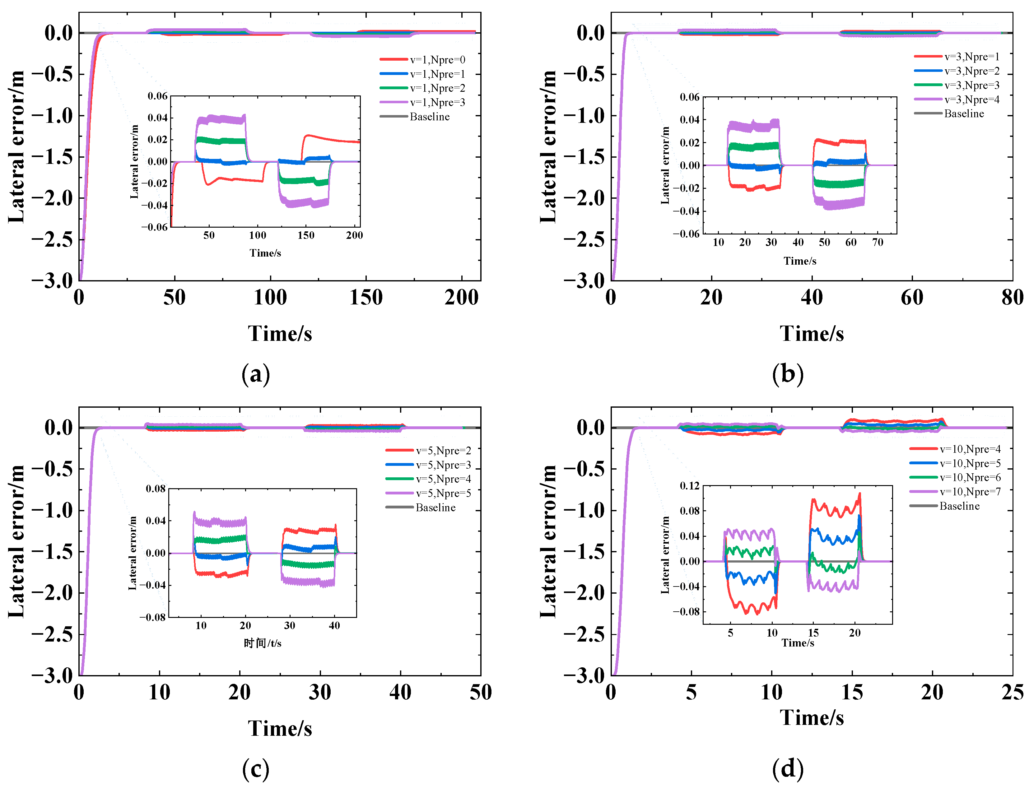
Impact of velocity on the value of N_pre

Take the U-shaped path (the commonly used agricultural machinery operation path) as the reference path and set N_p = 10 and N_c = 3.

Figure 7a illustrates that when v = 1 m/s, the tracking effect is ranked as N_pre(0) < N_pre(1) > N_pre(2) > N_pre(3), where N_pre = 1 indicates the tracking effect’s optimality. Figure 7b illustrates that when v = 3 m/s, the tracking effect is ranked as N_pre(1) < N_pre(2) > N_pre(3) > N_pre(4), where N_pre = 2 indicates the tracking effect’s optimality. Figure 7c illustrates that when v = 5 m/s, the tracking effect is ranked as N_pre(2) < N_pre(3) > N_pre(4) > N_pre(5), where N_pre = 3 indicates the tracking effect’s optimality. Figure 7d illustrates that when v = 10 m/s, the tracking effect is ranked as N_pre(4) < N_pre(5) < N_pre(6) > N_pre(7), where N_pre = 6 indicates the tracking effect’s optimality.

In summary, the selection of the value of N_pre is correlated positively with the curvature of the reference path and velocity.

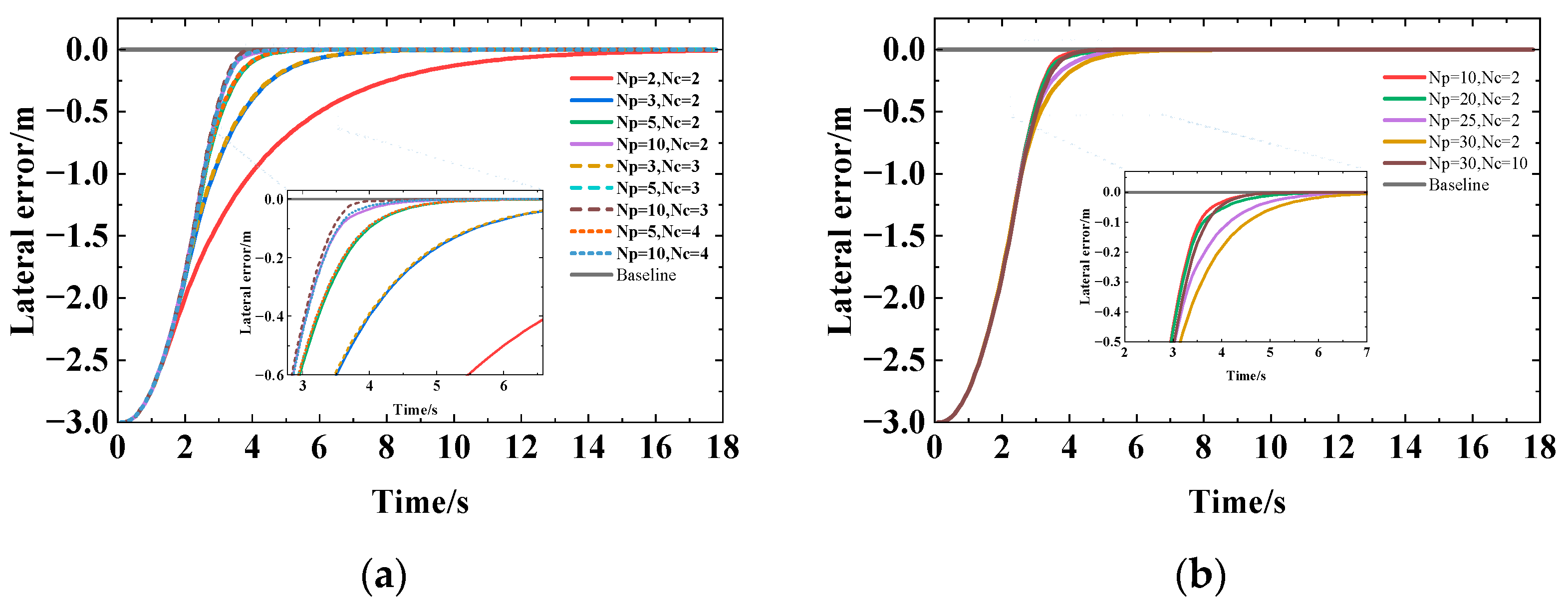
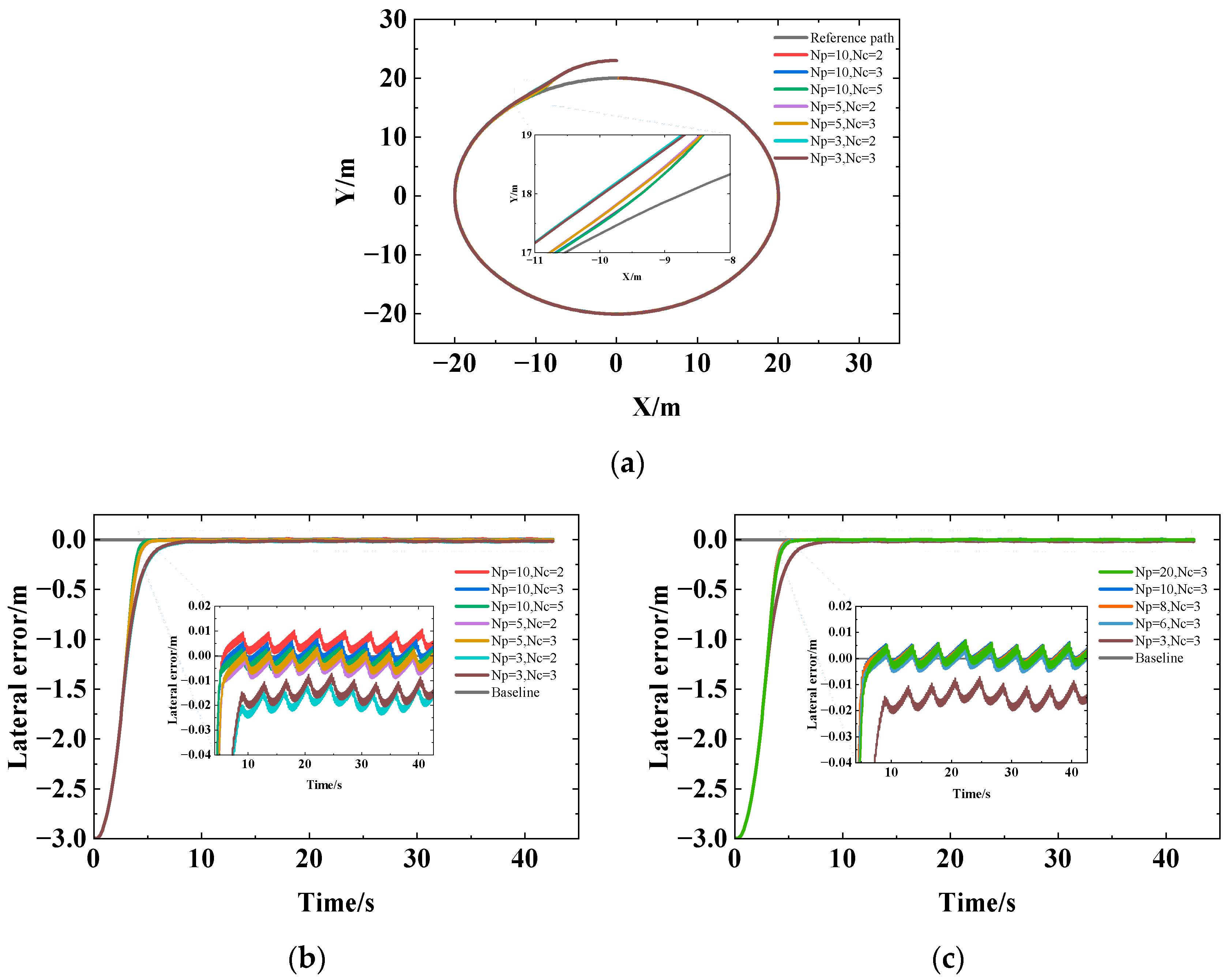
2.3.3. Impact of the Predictive Horizon and Control Horizon on Tracking Effect

(1) When tracking a straight path (set N_pre = 0)

As can be seen in Figure 8a, a smaller N_p corresponds to slower convergence and a bigger N_p to faster online time. The difference in the control effect is not significant when N_c = 2, 3, and 4. Nevertheless, considering real-time control, N_p should be appropriately increased and N_c reduced while tracking a straight path; the tracking effect is best where N_p = 10 and N_c = 2, as shown in Figure 8. But once N_p rises to a certain point, convergence slows down while N_c remains constant, necessitating simultaneous adjustments to N_p and N_c, as Figure 8b illustrates. Thus, N_p should be adjusted adequately but not excessively for straight path tracking.

(2) When tracking curves (set N_pre = 2)

In the case of the fixed-curvature circular path and the variable-curvature U-shaped path, as shown in Figure 9b and Figure 10b, the control effect is better at N_c = 3 than it is at N_c = 2 when N_p = 3, 5, 10, respectively. While as N_c increases (referring to N_c = 5), the control impact does not significantly alter. As a result, N_c can be increased suitably for curve tracking while taking the computation of the real-time performance into account. When N_p = 10 and N_c = 3, there is a better effect, as shown in the illustration.

The difference in tracking effect is not significant when N_p = 6, 8, 10, 20, respectively, as shown by Figure 9c and Figure 10c. Therefore, N_p can be suitably lowered considering the computational load and real-time computation when the curve is tracked. However, when it is reduced to a smaller value (referring to N_p = 3 and N_c = 3), the tracking effect is rather decreased.

In conclusion, the selection of N_p and N_c is affected by the reference path curvature ρ. N_p should be increased appropriately and N_c should be reduced appropriately when tracking a straight path. For curve tracking, N_p should be decreased appropriately to account for as much path curvature information as possible in each prediction horizon, and N_c should be increased appropriately to reduce the amplitude of changes in rear-wheel steering while ensuring tracking accuracy and stability.

At low vehicle speeds, the steering wheel needs to go a shorter distance to reach the target corner, resulting in a smaller total error during the process, while at high vehicle speeds, the vehicle will travel farther, potentially causing inferior tracking performance. Therefore, N_p should also grow when v increases to avoid the premature steering issue. N_c should also increase accordingly to reduce sudden changes in control inputs, preventing situations of skidding or even loss of control when driving at high speeds. The influence laws of reference path curvature ρ and vehicle speed v on N_p, N_c, and N_pre are summarized in

Table 3. The influence laws of ρ and v on N_p, N_c, and N_pre.

Parameters		Np	Nc	Npre
ρ	↑	↓	↑	↑
	↓	↑	↓	↓
v	↑	↑	↑	↑
	↓	↓	↓	↓

Note: ↑ represents positive correlation; ↓ represents negative correlation.

.

It is obvious that varying operation speeds and path curvatures result in different tracking performances. The impact of changes in reference path curvature and agricultural machinery operating speed on tracking performance is not taken into account by the conventional MPC algorithm, which has fixed N_p, N_c, and N_pre values. N_p, N_c, and N_pre can be dynamically adjusted based on the reference path curvature and operating speed to achieve parameter adaptation.

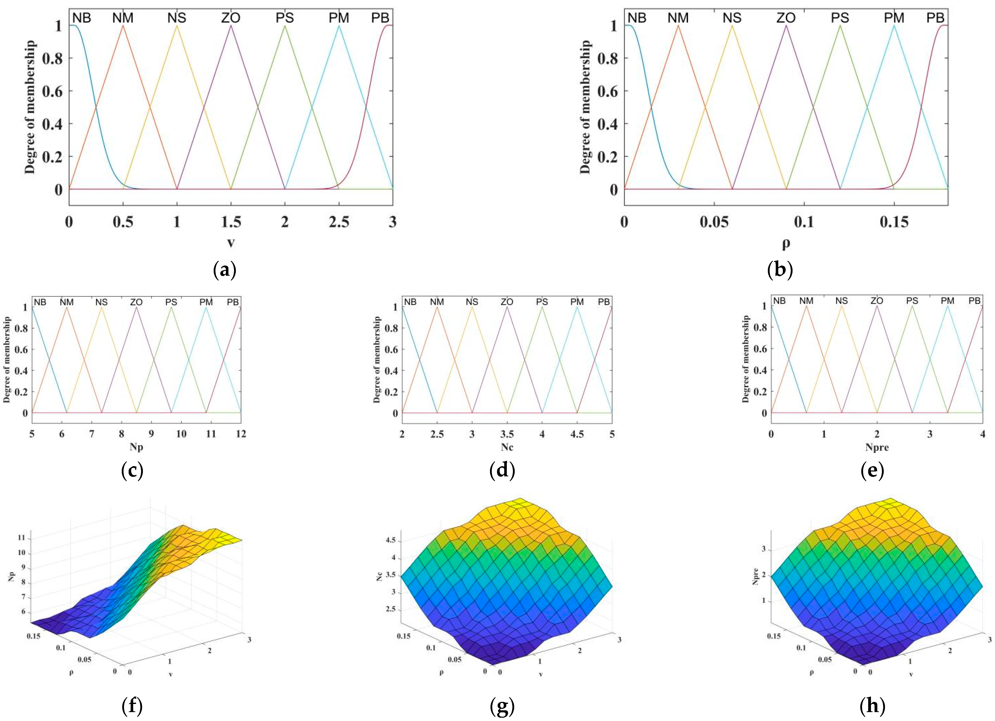
2.4. Parameter Adaptive MPC

2.4.1. Parameter Adaptive MPC Based on Fuzzy Control

Fuzzy control (FC) has the advantage of handling nonlinear factors and the effects of uncertainty. The primary idea is to create fuzzy rules based on expert experience, then fuzzify the input, apply fuzzy reasoning, and defuzzify the results to obtain accurate outcomes. It benefits from being simple in design, easy to implement and transplant, and independent of the mathematical models of the controlled object [28]. Therefore, fuzzy control can be employed to perform the adaptive adjustment of N_p, N_c, and N_pre, based on the analysis of affecting factors in Section 2.3. Use v and ρ as the input parameters, while N_p, N_c, and N_pre are the outputs to the fuzzy control, i.e., as follows:

$$[N_p,N_c,N_{pre}]=Round[Fuzzy(v,\rho )]$$

(22)

where Round represents the rounding function, and Fuzzy represents a fuzzy control function.

Classify v, ρ, N_p, N_c, and N_pre into 7 fuzzy subsets, respectively: NB, NM, NS, ZO, PS, PM, and PB. An optimization strategy for output variables was developed based on the simulation results, and a fuzzy control rule library was established using the Mamdani method.

Table 4. Fuzzy control rules and range of variable values.

Np = [5, 12]		v = [0, 3]
		NB	NM	NS	ZO	PS	PM	PB
ρ = [0, 0.18]	NB	ZO	PS	PM	PM	PB	PB	PB
	NM	NS	ZO	PS	PM	PM	PB	PB
	NS	NM	NS	ZO	PS	PM	PM	PB
	ZO	NM	NM	NS	ZO	PS	PM	PM
	PS	NB	NM	NM	NS	ZO	PS	PM
	PM	NB	NB	NM	NM	NS	ZO	PS
	PB	NB	NB	NB	NM	NM	NS	ZO
Nc = [2, 5]		v = [0, 3]
		NB	NM	NS	ZO	PS	PM	PB
ρ = [0, 0.18]	NB	NB	NB	NB	NM	NM	NS	ZO
	NM	NB	NB	NM	NM	NS	ZO	PS
	NS	NB	NM	NM	NS	ZO	PS	PM
	ZO	NM	NM	NS	ZO	PS	PM	PM
	PS	NM	NS	ZO	PS	PM	PM	PB
	PM	NS	ZO	PS	PM	PM	PB	PB
	PB	ZO	PS	PM	PM	PB	PB	PB
Npre = [0, 4]		v = [0, 3]
		NB	NM	NS	ZO	PS	PM	PB
ρ = [0, 0.18]	NB	NB	NB	NB	NM	NM	NS	ZO
	NM	NB	NB	NM	NM	NS	ZO	PS
	NS	NB	NM	NM	NS	ZO	PS	PM
	ZO	NM	NM	NS	ZO	PS	PM	PM
	PS	NM	NS	ZO	PS	PM	PM	PB
	PM	NS	ZO	PS	PM	PM	PB	PB
	PB	ZO	PS	PM	PM	PB	PB	PB

illustrates the fuzzy control rules and the range of values for each variable.

Figure 11 presents each variable’s membership functions and the fuzzy control surface. Gaussian membership functions were applied at both ends of the input variable domain and triangular membership functions were applied in the middle region of the domain to ensure high accuracy, stability, and sensitivity. The fuzzy outputs were obtained through fuzzy inference, and the precise output of N_p, N_c, and N_pre were obtained by using the MIN-MAX-Center of Gravity method for defuzzification.

2.4.2. Parameter Adaptive MPC Based on PSO

Particle Swarm Optimization (PSO) is a heuristic global search algorithm based on swarm intelligence, characterized by its ease of implementation, high accuracy, and rapid convergence [29]. The basic idea involves leveraging collaboration and information exchange among particles to arrive at the optimal solution [30].

The PSO algorithm first initializes n particles to form a population B = (B₁, B₂, …, B_n), where every particle stands for a possible ideal solution. The position and velocity of the i-th particle Bi are X_i = (x_i1, x_i2, …, x_id) and V_i = (v_i1, v_i2, …, v_id), respectively. Then, the particles update their position and velocity by tracking individual extremum P_best = (p_i1, p_i2, …, p_id) and population extremum G_best = (p_g1, p_g2, …, p_gd) during the iteration process. The updated formula is as follows:

$$\begin{array}{c}{V}_{id}^{k+1}=\omega V_{id}^k+c_1{r}_1(P_{id}^k-X_{id}^k)+c_2{r}_2(P_{gd}^k-X_{gd}^k)\\ X_{id}^{k+1}=X_{id}^k+V_{id}^{k+1}\end{array}$$

(23)

where ω is the inertia factor with a non-negative value; c₁ and c₂ are individual and group learning factors, respectively; and r₁ and r₂ are randomly generated numbers ranging from 0 to 1.

Local search benefits more from a smaller ω, while a bigger one is better for global search. Better optimization results can be achieved with the dynamic ω than with the fixed one, as it can better balance the capabilities of local and global search. This paper adopted the commonly used Linear Decreasing Weight (LDW) strategy, i.e., as follows:

$${\omega }_k=({\omega }_{\mathrm{int}}-{\omega }_{end})(G_k-k)/G_k+{\omega }_{end}$$

(24)

where G_k stands for the maximum number of iterations, k denotes the current iterations number, ${\omega }_{init}$ represents the initial inertia weight, and ${\omega }_{end}$ represents the inertia weight when evolving to the maximum iterations.

Set N_p, N_c, and N_pre as the three dimensions of each particle. Set the root mean square error of the lateral error as the fitness function, i.e., as follows:

$$Fitness(i)=MSE(e_d-r_{ed})$$

(25)

where Fitness represents the fitness function, MSE represents the root mean square error function, and r_ed represents the lateral error reference value.

Table 5. PSO parameter settings.

Parameters	Values
Particle dimension D	3
Pop size	1
Maximum number of iterations	100
Individual learning factor c1	0.8
Global learning factor c2	1
VarSize of Np	[5, 12]
VarSize of Nc	[2, 5]
VarSize of Npre	[0, 4]
ωinit	0.9
ωend	0.4

displays the key parameter settings of the PSO algorithm, and Figure 12 illustrates the control process.

3. Results and Discussion

3.1. Simulation Test Results

The tracking effects of the manual tuning MPC (MPC), the parameter adaptive MPC based on fuzzy control (FC_MPC), and the parameter adaptive MPC based on PSO (PSO_MPC) under U-shaped paths (commonly used operation paths) and complex curve paths (simulating curve driving and obstacle avoidance behaviors, etc.) were compared and analyzed through simulation.

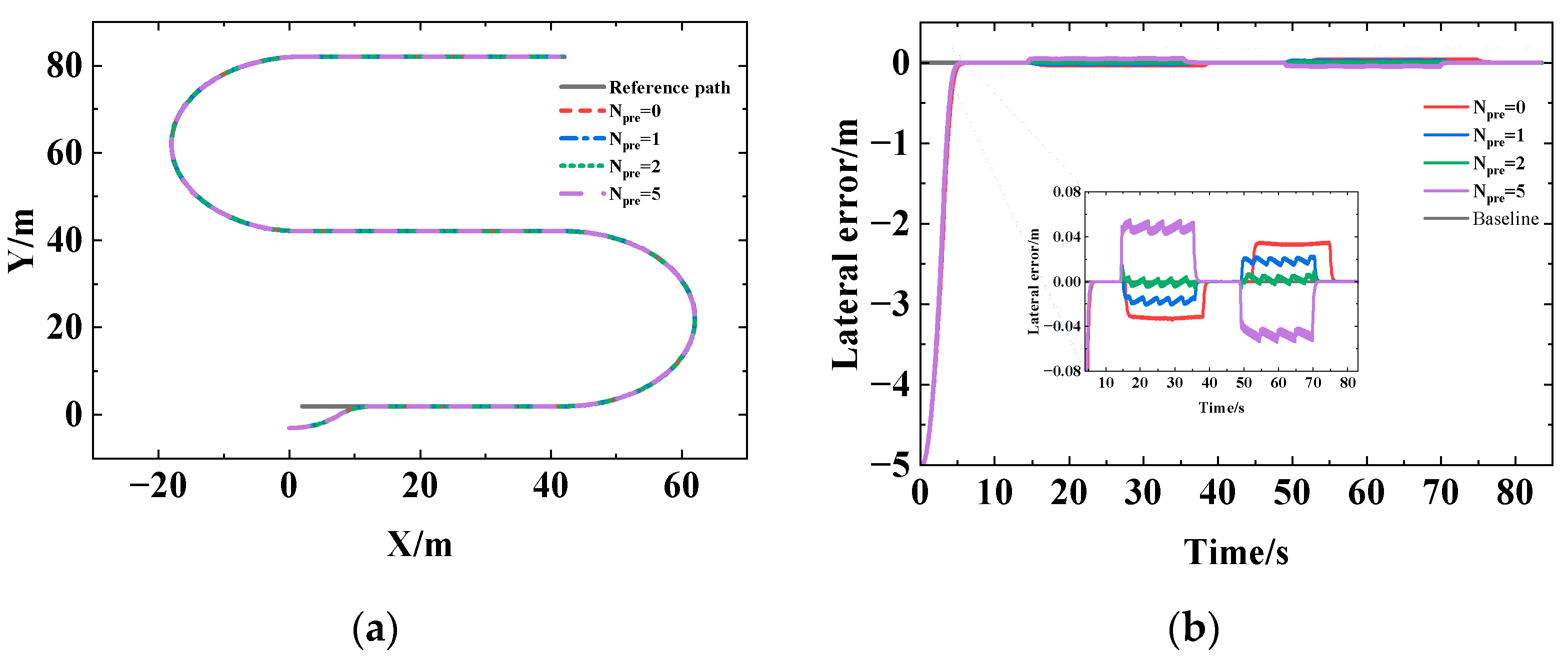
3.1.1. U-Shaped Path Simulation Test

Set N_p = 6, N_c = 3, and N_pre = 2 for the manual tuning MPC. From Figure 13 and

Table 6. Statistics of lateral and heading errors under U-shaped path tracking without disturbances.

Control Algorithm	Online Time /s	Online Distance/m	Absolute Value of Lateral Error			Absolute Value of Heading Error
			Mean Value /m	Standard Deviation /m	Maximum Error /m	Mean Value /rad	Standard Deviation /rad	Maximum Error /rad
MPC	4.1	11.29	0.0016	0.0023	0.0238	0.0096	0.0091	0.0325
FC_MPC	3.9	10.67	0.0014	0.0021	0.0214	0.0095	0.0091	0.0321
PSO_MPC	3.7	10.10	0.0003	0.0028	0.0168	0.0095	0.0091	0.0326

, the tracking effects of MPC, FC_MPC, and PSO_MPC differ little and all have superior tracking effects under no external disturbance. In contrast, the effect of PSO_MPC is slightly better than the first two. The mean absolute values of lateral errors for the three methods are 0.0016 m, 0.0014 m, and 0.0003 m, respectively, with maximum values of 0.0238 m, 0.0014 m, and 0.0168 m. The mean absolute values of heading errors for the three methods are 0.0096 rad, 0.0095 rad, and 0.0095 rad, respectively, with maximum values of 0.0325 rad, 0.0321 rad, and 0.0326 rad.

The tracking effects of FC_MPC and PSO_MPC are significantly better than that of MPC when the random perturbation of [1, 5] is set for the speed, as shown in Figure 14 and

Table 7. Statistics of lateral and heading errors under U-shaped path tracking with disturbances.

Control Algorithm	Online Time /s	Online Distance /m	Absolute Value of Lateral Error			Absolute Value of Heading Error
			Mean Value /m	Standard Deviation /m	Maximum Error /m	Mean Value /rad	Standard Deviation /rad	Maximum Error /rad
MPC_Disturb	2.1	11.67	0.0189	0.0181	0.0561	0.0060	0.0076	0.0502
FC_MPC_Disturb	1.9	9.93	0.0047	0.0059	0.0498	0.0160	0.0153	0.0471
PSO_MPC_Disturb	1.7	10.44	0.0049	0.0056	0.0244	0.0159	0.0151	0.0463

. There is a small difference between the two effects of FC_MPC and PSO_MPC, and the tracking effect is lower than when there is no perturbation but still within the usage demand range. The mean absolute values of lateral errors for the three methods are 0.0189 m, 0.0047 m, and 0.0049 m, respectively, with maximum values of 0.0561 m, 0.0498 m, and 0.0244 m. The mean absolute values of heading errors for the three methods are 0.0060 rad, 0.0160 rad, and 0.0159 rad, respectively, with maximum values of 0.0502 rad, 0.0471 rad, and 0.0463 rad.

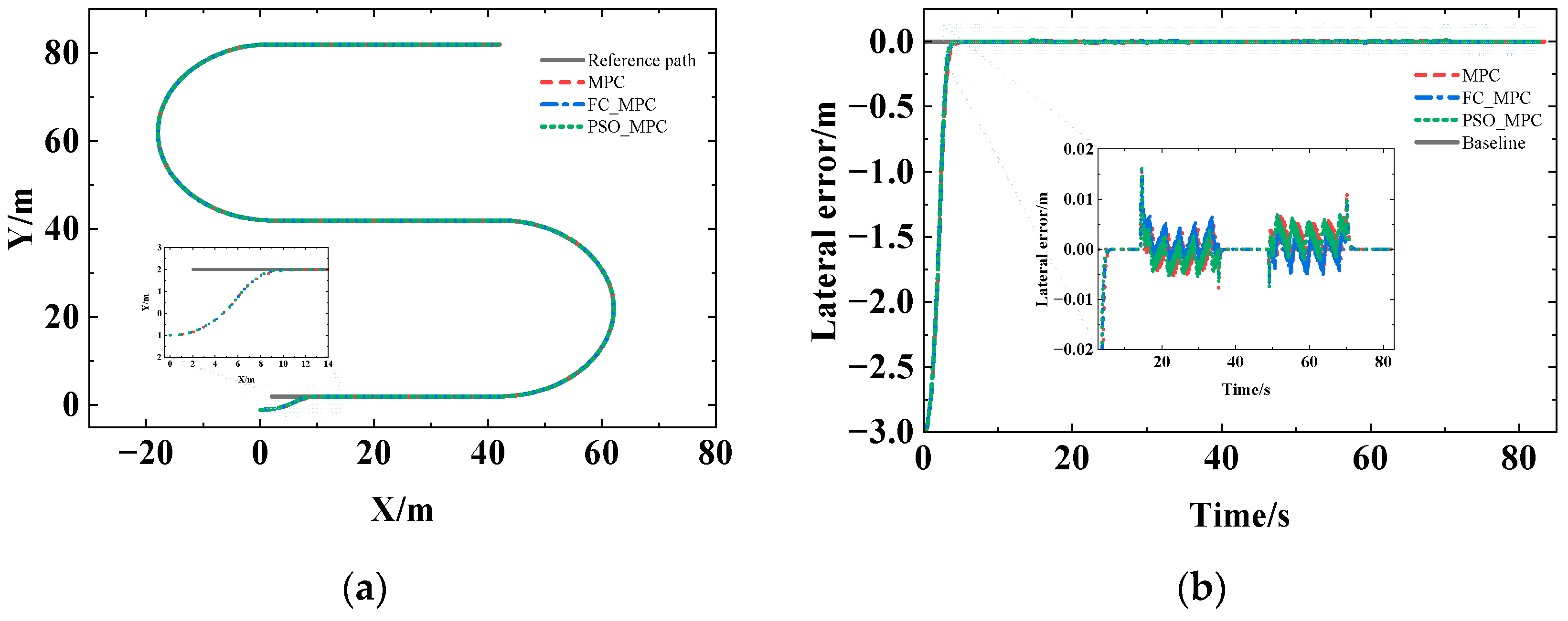
3.1.2. Complex Curve Path Simulation Test

Set N_p = 10, N_c = 3, and N_pre = 2 for the manual tuning MPC. As can be observed from Figure 15 and

Table 8. Statistics of lateral and heading errors under complex curve path tracking without disturbances.

Control Algorithm	Online Time /s	Online Distance/m	Absolute Value of Lateral Error			Absolute Value of Heading Error
			Mean Value /m	Standard Deviation /m	Maximum Error /m	Mean Value /rad	Standard Deviation /rad	Maximum Error /rad
MPC	4.2	10.57	0.0017	0.0035	0.0269	0.0021	0.0046	0.0334
FC_MPC	4.3	10.81	0.0018	0.0037	0.0315	0.0022	0.0046	0.0334
PSO_MPC	4.2	10.45	0.0016	0.0034	0.0290	0.0022	0.0046	0.0330

, similar to the U-shaped path, MPC, FC_MPC, and PSO_MPC differ little and all have good tracking effects under no external disturbance. The mean absolute values of lateral errors for the three methods are 0.0017 m, 0.0018 m, and 0.0019 m, respectively, with maximum values of 0.0269 m, 0.0315 m, and 0.0290 m. The mean absolute values of heading errors for the three methods are 0.0021 rad, 0.0022 rad, and 0.0022 rad, respectively, with maximum values of 0.0334 rad, 0.0334 rad, and 0.0330 rad.

Similar to the U-shaped path, the tracking effects of FC_MPC and PSO_MPC are significantly better than that of MPC when the random perturbation of [−5, 5] is set for the speed, as shown by Figure 16 and

Table 9. Statistics of lateral and heading errors in complex curve path tracking with disturbances.

Control Algorithm	Online Time /s	Online Distance/m	Absolute Value of Lateral Error			Absolute Value of Heading Error
			Mean Value /m	Standard Deviation /m	Maximum Error /m	Mean Value /rad	Standard Deviation /rad	Maximum Error /rad
MPC_Disturb	4.9	26.59	0.0072	0.0137	0.1625	0.0022	0.0046	0.0293
FC_MPC_Disturb	2.3	11.12	0.0020	0.0033	0.0200	0.0020	0.0033	0.0200
PSO_MPC_Disturb	2.3	13.14	0.0018	0.0031	0.0193	0.0021	0.0044	0.0263

. Furthermore, the difference in tracking performance between FC_MPC and PSO_MPC is relatively small. The mean absolute values of lateral errors for the three methods are 0.0072 m, 0.0020 m, and 0.0018 m, respectively, with maximum values of 0.1625 m, 0.0200 m, and 0.0193 m. The mean absolute values of heading errors for the three methods are 0.0022 rad, 0.0020 rad, and 0.0021 rad, respectively, with maximum values of 0.0293 rad, 0.0200 rad, and 0.0263 rad.

3.2. Discussion

According to the above simulation and analysis results, it can be seen that the three designed controllers, the manual tuning MPC, the FC_MPC, and the PSO_MPC, can achieve a better control effect under no disturbance, whether in the U-shaped path or complex curve path, meeting the requirements of ISO12188-2:2012(E) [31] and GB/T 37164-2018 [32] for agricultural machinery operation with a lateral error of less than 2.5 cm. This also demonstrates that, similar to PID parameter tuning, the MPC with manual parameter tuning under constant debugging can obtain the optimal key parameters combination, and that the control results satisfy the demand for control accuracy. Nevertheless, the debugging process is laborious, and the acquisition of debugging results has significant randomness and uncertainty. What is more, it lacks robustness and is not flexible enough to adjust to changing operating conditions. Due to the complex and ever-changing working environment of agricultural machinery, the FC_MPC and PSO_MPC with parameter adaptation designed in this paper have stronger applicability and application value.

The parameter adaptive MPC in this paper is based on the vehicle kinematic model, which is simple to control and can meet operational requirements, but it does not consider the effects of vehicle forces and ground conditions. Therefore, it is of certain research value and significance to design the parametric adaptive MPC controller based on the dynamic model of rear-wheel-steering vehicles (refer to Section 2.1.2), to compare and analyze the similarities and differences between the two in terms of the control effect, and to focus on summarizing the applicability conditions of the two, so as to make the controller’s control accuracy, stability, and adaptability higher.

4. Conclusions

To enhance the precision and adaptability of path tracking, based on establishing kinematic and dynamic models of rear-wheel-steering agricultural machinery and analyzing the factors affecting the tracking effect, this study proposed the adaptive parameters MPC based on fuzzy control and PSO. The main conclusions are as follows:

• Since the vehicle model is a vital part of implementing MPC, the kinematic and dynamic error state–space equations for rear-wheel-steering agricultural machinery were established, which can directly apply to the design of MPC controllers.
• The factors impacting the MPC control effect were simulated and analyzed using the kinematic model as the control model. (a) The larger the unique vehicle intrinsic physical quantity wheelbase incorporated by the kinematic model, the larger the online time and distance. (b) Increasing N_pre was favorable to improving the curve tracking effect, and N_pre was correlated positively with the curvature and speed changes. Preferred values of N_pre for the U-shaped path were 1, 2, 3, and 6, respectively, at speeds of 1 m/s, 3 m/s, 5 m/s, and 10 m/s. (c) The tracking effect was affected by the parameter settings of N_p and N_c, which were influenced by the curvature and speed. N_p should be increased appropriately and N_c should be decreased appropriately in straight path tracking, while N_p should be decreased appropriately and N_c should be increased appropriately in curve tracking. N_p and N_c should be increased appropriately when the vehicle speed increases.
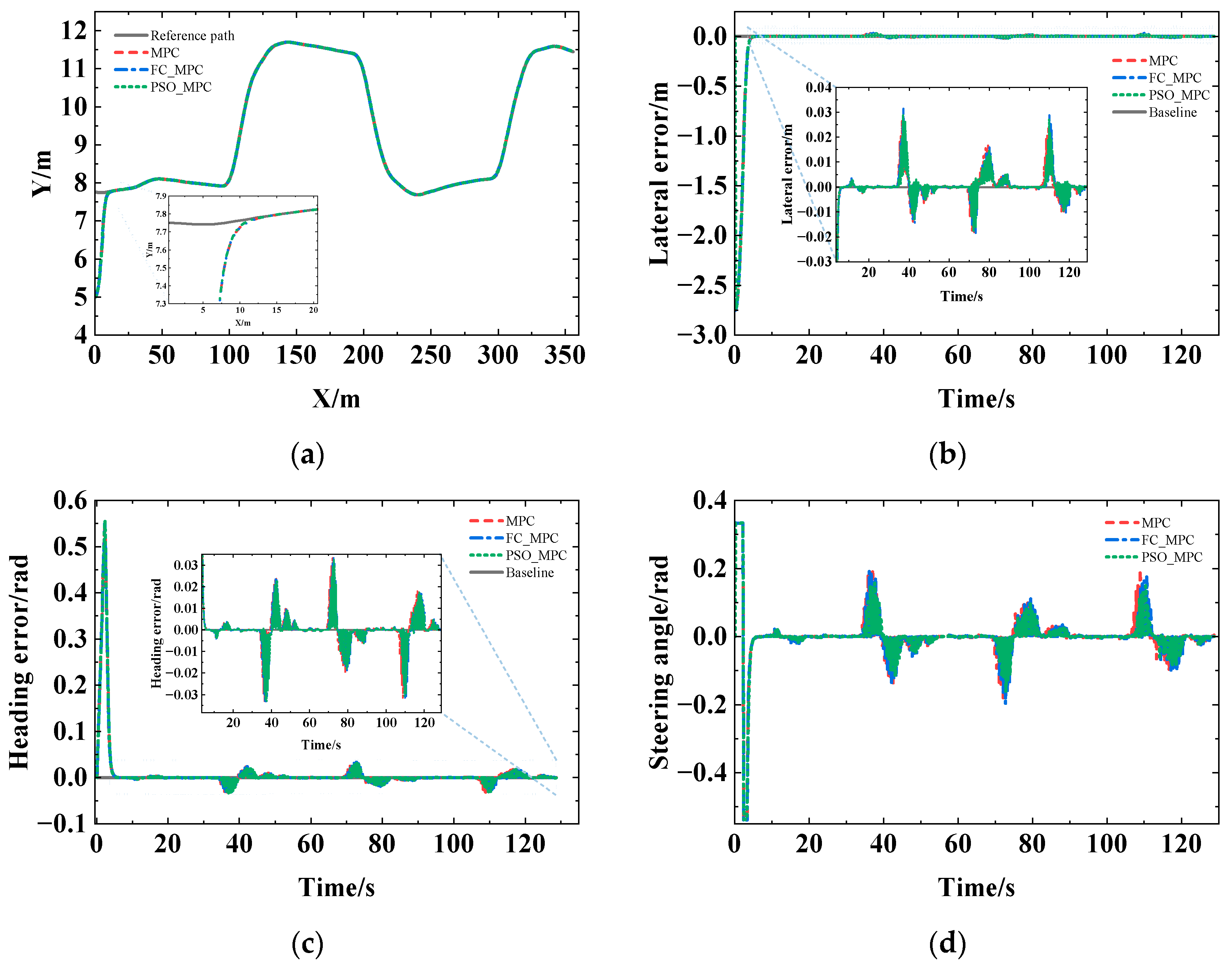
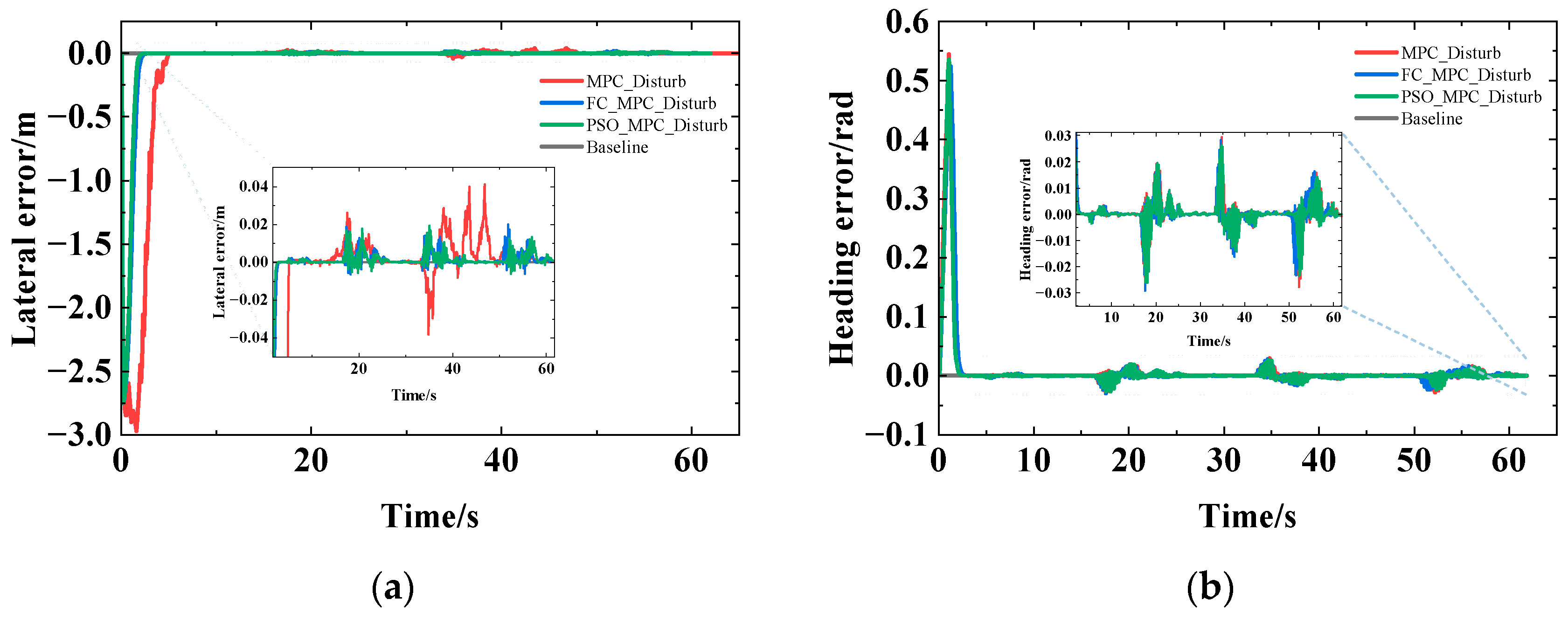
• Fuzzy control and the PSO algorithm were used to establish the adaptive MPC parameters (N_p, N_c, and N_pre) under different curvatures and velocities, and then the simulation platform was built based on MATLAB for simulation and analysis under U-shaped and complex curve paths. The results indicated that the differences among the manual tuning MPC, the FC_MPC, and the PSO_MPC were small under no disturbance, and the tracking effects were all better. The mean absolute value of lateral error was ≤0.0018 m, with the maximum error <0.0315 m, while the mean absolute value of heading error was ≤0.0096 rad, with the maximum error <0.0325 rad. Laterally, this implies that manual tuning can obtain an optimal parameters combination, but with high uncertainty and low efficiency. The tracking effect of FC_MPC and PSO_MPC was significantly better than that of the manual tuning MPC under random velocity disturbance, and the difference between FC_MPC and PSO_MPC was not significant. As a result, FC_MPC and PSO_MPC are more anti-interference compared to the manual tuning MPC with fixed horizon, and more adaptable to complex field scenarios.

References

1. Luo, X.; Liao, J.; Hu, L.; Zhou, Z.; Zhang, Z.; Zang, Y.; Wang, P.; He, J. Research progress of intelligent agricultural machinery and practice of unmanned farm in China. J. South China Agric. Univ. 2021, 42, 8–17+5. [Google Scholar]
2. Meng, Z.; Wang, H.; Fu, W.; Liu, M.; Yin, Y.; Zhao, C. Research Status and Prospects of Agricultural Machinery Autonomous Driving. Trans. Chin. Soc. Agric. Mach. 2023, 54, 1–24. [Google Scholar]
3. Macenski, S.; Singh, S.; Martín, F.; Ginés, J. Regulated Pure Pursuit for Robot Path Tracking. Auton. Robot. 2023, 47, 685–694. [Google Scholar] [CrossRef]
4. Wang, L.; Zhai, Z.; Zhu, Z.; Mao, E. Path Tracking Control of an Autonomous Tractor Using Improved Stanley Controller Optimized with Multiple-Population Genetic Algorithm. Actuators 2022, 11, 22. [Google Scholar] [CrossRef]
5. Han, G.; Fu, W.; Wang, W.; Wu, Z. The Lateral Tracking Control for the Intelligent Vehicle Based on Adaptive PID Neural Network. Sensors 2017, 17, 1244. [Google Scholar] [CrossRef] [PubMed]
6. Lee, K.; Jeon, S.; Kim, H.; Kum, D. Optimal Path Tracking Control of Autonomous Vehicle: Adaptive Full-State Linear Quadratic Gaussian (LQG) Control. IEEE Access 2019, 7, 109120–109133. [Google Scholar] [CrossRef]
7. Li, J.; Shang, Z.; Li, R.; Cui, B. Adaptive Sliding Mode Path Tracking Control of Unmanned Rice Transplanter. Agriculture 2022, 12, 1225. [Google Scholar] [CrossRef]
8. Wang, M.; Chen, J.; Yang, H.; Wu, X.; Ye, L. Path Tracking Method Based on Model Predictive Control and Genetic Algorithm for Autonomous Vehicle. Math. Probl. Eng. 2022, 2022, e4661401. [Google Scholar] [CrossRef]
9. Arifin, B.; Suprapto, B.Y.; Prasetyowati, S.A.D.; Nawawi, Z. Steering Control in Electric Power Steering Autonomous Vehicle Using Type-2 Fuzzy Logic Control and PI Control. World Electr. Veh. J. 2022, 13, 53. [Google Scholar] [CrossRef]
10. Li, H.; Gao, F.; Zuo, G. Research on the Agricultural Machinery Path Tracking Method Based on Deep Reinforcement Learning. Sci. Program. 2022, 2022, e6385972. [Google Scholar] [CrossRef]
11. Zhang, S.; Wang, H.; Chen, P.; Zhang, X.; Li, Q. Overview of the application of neural networks in the motion control of unmanned vehicles. Chin. J. Eng. 2022, 44, 235–243. [Google Scholar]
12. A Survey on Industry Impact and Challenges Thereof [Technical Activities]. IEEE Control Syst. 2017, 37, 17–18. [CrossRef]
13. Liu, J.; Yang, Z.; Huang, Z.; Li, W.; Dang, S.; Li, H. Simulation Performance Evaluation of Pure Pursuit, Stanley, LQR, MPC Controller for Autonomous Vehicles. In Proceedings of the 2021 IEEE International Conference on Real-time Computing and Robotics (RCAR), Xining, China, 15–19 July 2021; pp. 1444–1449. [Google Scholar]
14. Diaz-del-Rio, F.; Sanchez-Cuevas, P.; Iñigo-Blasco, P.; Sevillano-Ramos, J.L. Improving Tracking of Trajectories through Tracking Rate Regulation: Application to UAVs. Sensors 2022, 22, 9795. [Google Scholar] [CrossRef]
15. Xue, P.; Wu, Y.; Yin, G.; Liu, S.; Shi, Y. Path Tracking of Orchard Tractor Based on Linear Time-Varying Model Predictive Control. In Proceedings of the 2019 Chinese Control And Decision Conference (CCDC), Nanchang, China, 3–5 June 2019; pp. 5489–5494. [Google Scholar]
16. He, J.; Hu, L.; Wang, P.; Liu, Y.; Man, Z.; Tu, T.; Yang, L.; Li, Y.; Yi, Y.; Li, W.; et al. Path Tracking Control Method and Performance Test Based on Agricultural Machinery Pose Correction. Comput. Electron. Agric. 2022, 200, 107185. [Google Scholar] [CrossRef]
17. Zhou, B.; Su, X.; Yu, H.; Guo, W.; Zhang, Q. Research on Path Tracking of Articulated Steering Tractor Based on Modified Model Predictive Control. Agriculture 2023, 13, 871. [Google Scholar] [CrossRef]
18. Wang, H.; Liu, B.; Ping, X.; An, Q. Path Tracking Control for Autonomous Vehicles Based on an Improved MPC. IEEE Access 2019, 7, 161064–161073. [Google Scholar] [CrossRef]
19. Shi, P.; Chang, H.; Wang, C.; Ma, Q.; Zhou, M. Research on Path Tracking Control of Autonomous Vehicles Based on PSO-BP Optimized MPC. Automob. Technol. 2023, 7, 38–46. [Google Scholar]
20. Guan, L.; Liao, P.; Wang, A.; Shi, L.; Zhang, C.; Wu, X. Path tracking control of intelligent vehicles via a speed-adaptive MPC for a curved lane with varying curvature. Proc. Inst. Mech. Eng. Part D J. Automob. Eng. 2024, 238, 802–824. [Google Scholar] [CrossRef]
21. Liang, J.; Zhu, F.; Cai, Y.; Chen, X.; Chen, L. Intelligent Vehicle Path Tracking Control Based on Complex Curvature Variation. Automot. Eng. 2021, 43, 1771–1779. [Google Scholar]
22. Lin, X.; Tang, Y.; Zhou, B. Improved Model Predictive Control Path Tracking Strategy Based on an Online Updating Algorithm With Cosine Similarity and a Horizon Factor. IEEE Trans. Intell. Transp. Syst. 2022, 23, 12429–12438. [Google Scholar] [CrossRef]
23. Dai, C.; Zong, C.; Chen, G. Path Tracking Control Based on Model Predictive Control With Adaptive Preview Characteristics and Speed-Assisted Constraint. IEEE Access 2020, 8, 184697–184709. [Google Scholar] [CrossRef]
24. Choi, Y.; Lee, W.; Yoo, J. A Variable Horizon Model Predictive Control Based on Curvature Properties of Vehicle Driving Path. Trans. KSAE 2021, 29, 1147–1159. [Google Scholar] [CrossRef]
25. Liu, H.; Sun, J.; Cheng, K.W.E. A Two-Layer Model Predictive Path-Tracking Control With Curvature Adaptive Method for High-Speed Autonomous Driving. IEEE Access 2023, 11, 89228–89239. [Google Scholar] [CrossRef]
26. Jing, L.; Zhang, Y.; Shen, Y.; He, S.; Liu, H.; Cui, Y. Adaptive Trajectory Tracking Control of 4WID High Clearance Unmanned Sprayer. Trans. Chin. Soc. Agric. Mach. 2021, 52, 408–416. [Google Scholar]
27. Shen, Y.; Zhang, Y.; Liu, H.; He, S.; Feng, R.; Wan, Y. Research Review of Agricultural Equipment Automatic Control Technology. Trans. Chin. Soc. Agric. Mach. 2023, 54, 1–18. [Google Scholar]
28. Belman-Flores, J.M.; Rodríguez-Valderrama, D.A.; Ledesma, S.; García-Pabón, J.J.; Hernández, D.; Pardo-Cely, D.M. A Review on Applications of Fuzzy Logic Control for Refrigeration Systems. Appl. Sci. 2022, 12, 1302. [Google Scholar] [CrossRef]
29. Gad, A.G. Particle Swarm Optimization Algorithm and Its Applications: A Systematic Review. Arch. Comput. Methods Eng. 2022, 29, 2531–2561. [Google Scholar] [CrossRef]
30. Li, D.; Wang, L.; Guo, W.; Zhang, M.; Hu, B.; Wu, Q. A Particle Swarm Optimizer with Dynamic Balance of Convergence and Diversity for Large-Scale Optimization. Appl. Soft Comput. 2023, 132, 109852. [Google Scholar] [CrossRef]
31. ISO 12188-2:2012(E); Tractors and Machinery for Agriculture and Forestry-Test Procedures for Positioning and Guidance Systems in Agriculture-Part 2: Testing of Satellite-Based Auto-Guidance Systems during Straight and Level Travel. International Organization for Standardization: Geneva, Switzerland, 2012.
32. GB/T 37164-2018; Work Performance Requirements and Evaluation Method of Auto-Guidance Systems for Self-Propelled Agricultural Machinery. State Administration for Market Regulation. China National Standardization Administration: Beijing, China, 2018.
Figure 1. Schematic diagram of the kinematic model for agricultural machinery. Note: φ is the yaw angle; β is the center of mass lateral deviation angle; L is the wheelbase; v is the center of mass velocity; δf and δr are front- and rear-wheel angles, respectively; and R is the instantaneous turning radius.
Agriculture 14 00823 g001
Figure 2. Schematic diagram of 2DoF dynamic model for rear-wheel-steering agricultural machinery. Note: Flf and Flr are the longitudinal forces acting on the front and rear wheels; Fcf and Fcr are the lateral forces acting on the front and rear wheels; Fxf and Fxr are the combined forces acting on the front and rear wheels along the x-axis; Fyf and Fyr are the combined forces acting on the front and rear wheels along the y-axis; vx and vy are the longitudinal and lateral velocities of the vehicle; lf and lr are the distances between the front and rear axles and the center of mass, respectively; θvr is the velocity deviation angle of the rear wheels.
Agriculture 14 00823 g002
Figure 3. Tracking effects with different wheelbases under straight paths. (a) Path tracking; (b) lateral error; (c) heading error; (d) rear-wheel steering angle.
Agriculture 14 00823 g003
Figure 4. Schematic diagram of lateral error calculation.
Agriculture 14 00823 g004
Figure 5. U-shaped path-tracking effect under different values of Npre. (a) Path tracking; (b) lateral error.
Agriculture 14 00823 g005
Figure 6. Effect of double-lane change path tracking at different values of Npre. (a) Path tracking; (b) lateral error.
Agriculture 14 00823 g006
Figure 7. Lateral error under different Npre values at different velocities. (a) Lateral error under different Npre values at v = 1 m/s; (b) lateral error under different Npre values at v = 3 m/s; (c) lateral error under different Npre values at v = 5 m/s; (d) lateral error under different Npre values at v = 10 m/s.
Agriculture 14 00823 g007
Figure 8. Lateral error under different Np and Nc values of straight path tracking. (a) Lateral error I; (b) lateral error II.
Agriculture 14 00823 g008
Figure 9. Circular path-tracking effect under different Np and Nc values. (a) Path tracking; (b) lateral error I; (c) lateral error II.
Agriculture 14 00823 g009
Figure 10. U-shaped path-tracking effect under different Np and Nc values (a) Path tracking; (b) lateral error I; (c) lateral error II.
Agriculture 14 00823 g010
Figure 11. Relationship of input and output variables. (a) Membership function of v; (b) membership function of ρ; (c) membership function of Np; (d) membership function of Nc; (e) membership function of Npre; (f) fuzzy control surface of Np; (g) fuzzy control surface of Nc; (h) fuzzy control surface of Npre.
Agriculture 14 00823 g011
Figure 12. PSO-MPC control flow.
Agriculture 14 00823 g012
Figure 13. Contrast in tracking effects under a U-shaped path without disturbances. (a) Path tracking; (b) lateral error; (c) heading error; (d) rear-wheel steering angle.
Agriculture 14 00823 g013aAgriculture 14 00823 g013b
Figure 14. Comparison of tracking effects under a U-shaped path with disturbances. (a) Lateral error; (b) heading error.
Agriculture 14 00823 g014
Figure 15. Contrast in tracking effects under complex curve path without disturbances. (a) Path tracking; (b) lateral error; (c) heading error; (d) rear-wheel steering angle.
Agriculture 14 00823 g015
Figure 16. Contrast in tracking effects under complex curve path with disturbances. (a) Lateral error; (b) heading error.
Agriculture 14 00823 g016