Article

Advancing Cassava Age Estimation in Precision Agriculture: Strategic Application of the BRAH Algorithm

by
Sornkitja Boonprong
1,*,
Tunlawit Satapanajaru
2 and
Ngamlamai Piolueang
1
1
Faculty of Social Sciences, Kasetsart University, Bangkok 10900, Thailand
2
Faculty of Environment, Kasetsart University, Bangkok 10900, Thailand
*
Author to whom correspondence should be addressed.
Agriculture 2024, 14(7), 1075; https://doi.org/10.3390/agriculture14071075
Submission received: 9 May 2024 / Revised: 30 June 2024 / Accepted: 2 July 2024 / Published: 4 July 2024
(This article belongs to the Special Issue Precision Remote Sensing and Information Detection in Agriculture)

Abstract

:
Cassava crop age estimation is crucial for optimizing irrigation, fertilization, and pest management, which are key components of precision agriculture. Accurate knowledge of crop age allows for effective resource application, minimizing environmental impact and enhancing yield predictions. The Bare Land Referenced Algorithm from Hyper-Temporal Data (BRAH) is used for bare land classification and cassava crop age estimation, but it traditionally requires manual NDVI thresholding, which is challenging with large datasets. To address this limitation, we propose automating the thresholding process using Otsu’s method and enhancing the image contrast with histogram equalization. This study applies these enhancements to the BRAH algorithm for bare land classification and cassava crop age estimation in Ratchaburi, Thailand, utilizing a dataset of 604 Landsat satellite images from 1987 to 2024. Our research demonstrates the accuracy and practicality of the BRAH algorithm, with Otsu’s method providing 94% accuracy in detecting the bare land validation locations with an average deviation of 8.78 days between the acquisition date and the validated date. This approach facilitates precise agricultural planning and management, promoting sustainable farming practices and supporting several Sustainable Development Goals (SDGs).

1. Introduction

1.1. Crop Age Estimation in Precision Agriculture

According to the International Society of Precision Agriculture (ISPA), precision agriculture is defined as “a management strategy that gathers, processes, and analyzes temporal, spatial, and individual plant and animal data and combines it with other information to support management decisions according to estimated variability for improved resource use efficiency, productivity, quality, profitability, and sustainability of agricultural production” [1]. It crucially incorporates crop age estimation, providing farmers with essential information to optimize irrigation, fertilization, and pest management practices. Accurate knowledge of crop age allows for the effective application of resources, minimizing environmental impact and waste. This precision not only ensures the efficient use of fertilizers and water but also enhances yield predictions, facilitating the harvesting of crops at their economic peak while enabling early detection of diseases and pests. Such meticulous monitoring of crop age significantly contributes to healthier soil management practices and supports agricultural sustainability [2].
Precision agriculture directly contributes to SDG 2 (Zero Hunger) by enhancing productivity and reducing waste through meticulous crop age monitoring, which fine-tunes the use of irrigation, fertilizers, and pesticides. This targeted approach not only minimizes environmental degradation but also fosters sustainable agricultural practices. By adjusting resource application to the specific needs of crops at different growth stages, this method helps prevent soil degradation, reduces chemical runoff, and maintains soil health, enabling the production of more food with fewer resources and aligning with global food security objectives [3]. Furthermore, precision agriculture aids in achieving SDG 13 (Climate Action) by using crop age data to inform reforestation strategies that enhance carbon sequestration [4]. It also supports SDG 15 (Life on Land) through monitoring land cover age to prevent deforestation and manage ecosystems sustainably. Additionally, SDG 12 (Responsible Consumption and Production) is realized through the optimized application of resources, curtailing unnecessary chemical usage, and advancing sustainable practices. Advanced data analytics are now indispensable in agriculture, offering predictive insights that allow farmers to adjust their planting schedules and resource allocations based on forecasted weather, thus maximizing yields and minimizing losses. This data-driven approach not only refines the application of water, fertilizers, and pesticides but also aligns production with market demands, enhancing profitability and supply chain efficiency. Early detection of pests and diseases through data analytics facilitates rapid interventions, averting extensive damage and securing harvests, thus proving essential for navigating modern agricultural challenges and reinforcing global food security.
Recent advancements in agricultural monitoring and age estimation techniques have leveraged various machine learning and remote sensing approaches to improve accuracy and efficiency. Chumkesornkulkij et al. (2013) utilized an extended Kalman filter (EKF) on MODIS NDVI time-series data to estimate rice cultivation dates, achieving high accuracy for both rain-fed and irrigated areas. This method demonstrated the potential of using temporal data for precise crop monitoring, although it was limited by the moderate spatial resolution of MODIS data [5]. Chen et al. (2018) introduced an integrated pixel- and object-based tree growth model using annual Landsat time-series data to estimate the age of rubber plantations. This approach effectively reduced spectral noise and demonstrated robustness against data uncertainties, achieving high identification accuracy and a low average error in age estimation. The study underscored the value of combining pixel-based and object-based analyses for fine-scale age estimation in plantation monitoring [6]. Moreover, Baker (2003) compared the crown class model and the periodic annual increment (PAI) model for estimating the age of tropical trees. The crown class model, which stratifies growth rates by crown class, was found to be more accurate for shade-intolerant species, while the PAI model was better suited for shade-tolerant species. This research highlighted the importance of species-specific models and independent validation for accurate age estimation [7]. Furthermore, Agustin et al. (2020) employed convolutional neural networks (CNN) to classify the ages of oil palm plantations using Ikonos Panchromatic imagery. The study achieved high classification accuracy, particularly with the VGG19 pre-trained network, demonstrating the efficacy of deep learning in handling large-scale images with complex backgrounds. However, the high computational requirements and the need for high-resolution imagery were notable constraints [8]. Recently, Madugundu et al. (2024) utilized the random forest (RF) algorithm on Sentinel-2 imagery to determine the optimal timing for carrot crop monitoring and yield assessment. By integrating various vegetation indices and chlorophyll content, the study identified the best monitoring window for yield prediction between 60 and 75 days after planting (DAP), demonstrating high accuracy. This method provided a practical approach for sustainable carrot production, albeit requiring frequent and high-resolution imagery [9].

1.2. Global Importance of Cassava

Cassava stands as a fundamental global crop, sustaining the livelihoods of millions of smallholder farmers and serving as a primary carbohydrate source for over 800 million people across Africa, Asia, and Latin America [10]. Its resilience in poor soils and under drought conditions renders it indispensable in challenging climates. The high starch content of cassava permits its use in diverse industrial applications, including textiles, adhesives, biodegradable plastics, and biofuels, with Thailand noted as a leading exporter of tapioca starch, emphasizing cassava’s vital role in its agricultural economy [3].
However, cassava faces significant challenges, such as cassava mosaic disease (CMD), cassava brown streak disease (CBSD), fluctuating market demands, and soil degradation, all of which threaten its sustainability and productivity. To combat these issues, certain strategies, like breeding disease-resistant varieties, have been employed effectively against CMD and CBSD. Leveraging precision agriculture with remote sensing and IoT devices offers real-time insights into crop health, enabling timely interventions. Diversifying cassava products and adopting sustainable agronomic practices are crucial for maintaining soil health and enhancing the crop’s resilience. Additionally, improving market access, ensuring pricing transparency, and providing financial support are essential in empowering farmers to stabilize their incomes and increase resilience against external shocks. These comprehensive measures are critical for securing the future of cassava cultivation and ensuring it continues to make significant contributions to food security and economic stability [3,11].

1.3. Role of Cassava in Thailand

In Ratchaburi, a province in western Thailand with favorable climate and soil conditions, cassava farming significantly supports the livelihoods of smallholder farmers, ensuring a steady income through both domestic consumption and export markets. The resilience of cassava to climatic changes not only secures food security in the region but also underscores its role in bolstering agricultural sustainability by adapting to variable environmental conditions. The local processing industries in these regions transform raw cassava into a variety of value-added products, such as tapioca starch and animal feed, generating employment and stimulating the local economy by catering to both domestic and international markets. This economic activity enhances regional economic stability and contributes to the national GDP. Complementing these efforts, ongoing research and development initiatives led by institutions, like the Thai Tapioca Development Institute and the National Economic and Social Development Council, focus on developing disease-resistant cassava varieties, improving crop yields, and exploring innovative cassava-based products.

1.4. Recent Advances in Precision Agriculture for Cassava Cultivation

Recent research emphasizes the critical role of innovative agricultural practices and technologies in enhancing sustainability and resilience against environmental challenges, particularly in cassava cultivation. Manganyi et al. (2023) discuss the importance of sustainable practices, such as crop diversification and organic fertilization in cassava farming, which are crucial for maintaining soil health and biodiversity. They further emphasize the benefits of precision agriculture technologies in optimizing resource use and reducing waste in cassava cultivation. The authors argue that significant policy changes, enhanced educational opportunities for farmers, and substantial technological investments are necessary to achieve long-term food security and protect ecosystems [12]. Addressing broader agricultural challenges, Madugundu et al. (2024) propose a machine learning-based model for predictive maintenance in crop production, utilizing ensemble methods to optimize carrot crop monitoring and yield assessment with Sentinel-2 satellite data. This method significantly reduces operational costs and minimizes losses due to equipment failures [9]. Similarly, Han et al. (2023) developed a convolutional neural network (CNN) that efficiently detects mechanical faults in greenhouse farming machinery, enhancing fault detection speed and accuracy while reducing maintenance costs [13]. The vulnerabilities of rain-fed agriculture to climate change, as explored by Onyeneke et al. (2023), necessitate the adoption of climate-smart farming practices, such as improved irrigation systems and drought-resistant crops, which are also pertinent to cassava farming. These practices enhance resilience and are supported by comprehensive policy frameworks that promote farmer education and regional cooperation [14]. Olarinde et al. (2020) further investigate the socioeconomic impacts of climate change on cassava farmers, recommending the adoption of climate-resilient crop varieties, better irrigation techniques, and proactive adaptation strategies to mitigate adverse effects [15].

1.5. The Current Study

The BRAH (Bare Land Referenced Algorithm from Hyper-Temporal Data) algorithm [2] utilizes hyper-temporal satellite imagery to monitor bare land states and track subsequent vegetation growth, particularly enhancing land cover change detection. By harnessing high-resolution temporal data, it identifies subtle vegetation changes, which is crucial for providing accurate crop age estimates. This method can be especially effective in classifying the age of cassava plantations due to its ability to capture distinctive multi-temporal growth patterns. Moreover, the BRAH algorithm leverages this detailed satellite data to offer insights into the progression of crop growth stages. Its capability to detect day or month changes in vegetation allows for precise age classification, making it highly suitable for cassava age estimation. This leads to improved accuracy in age determination, directly translating into enhanced crop management and optimized resource allocation.
In this article, we present significant enhancements to the original BRAH algorithm by integrating Otsu’s algorithm, tailored to efficiently handle large satellite datasets comprising 604 images spanning from 1987 to 2024. This refined approach introduces an effective workflow designed to accurately determine crop age. By utilizing advanced data science tools and image processing techniques within this framework, we aim to produce results that can significantly enhance the sustainability and future-readiness of agricultural practices. This advanced methodology not only streamlines the processing of extensive temporal datasets but also provides precise crop age estimates, which can be subsequently used to implement precision agriculture techniques. These techniques facilitate more informed, sustainable management decisions, ultimately driving forward the precision agriculture agenda.

2. Materials and Methods
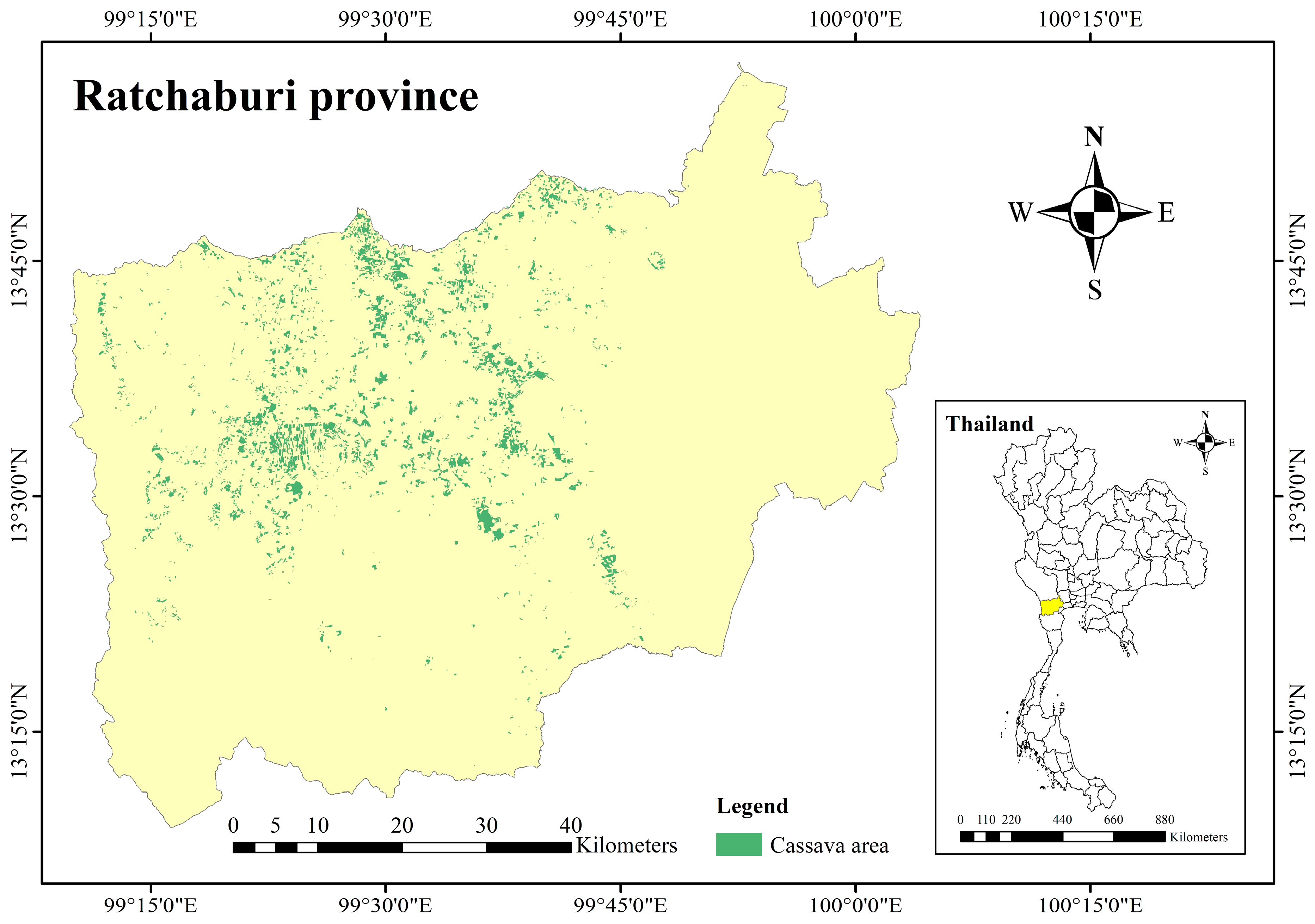
2.1. Study Sites

Ratchaburi Province (Figure 1), situated in western Thailand and covering an area of approximately 5196 square kilometers, is located at approximately 13.5264° N latitude and 99.8135° E longitude. This province presents a diverse landscape marked by rugged mountains in the west and expansive river plains traversed by the Mae Klong River. Within this region, a variety of ecosystems thrive, including dense forests and fertile wetlands, supporting a rich array of flora and fauna. Its subtropical climate brings distinct seasonal variations, with warm and humid summers contrasting with cooler winters. Ratchaburi plays a significant role in Thailand’s agricultural sector, particularly in cassava cultivation, benefiting from its favorable climate and fertile soils.

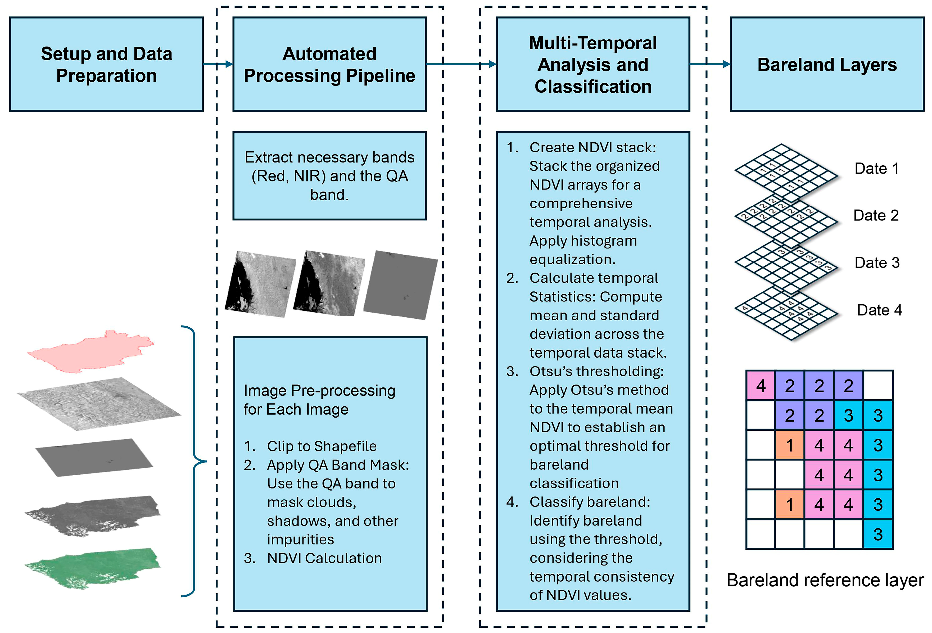
2.2. Data and Proprocessing

For this research, a comprehensive dataset of Landsat imagery spanning from 1987 to 2024 was utilized. The dataset comprises 604 Level-2 Collection 2 Tier 1 images from Landsat 4, 5, 7, 8, and 9, covering Ratchaburi Province as described in Table 1, Thailand. Notably, only Landsat 7 images prior to the 2003 sensor malfunction were incorporated to ensure uniform data quality. All images were downloaded from the EarthExplorer portal of the USGS.
To provide a comprehensive understanding of the temporal distribution of our satellite images, we have visualized the acquisition dates. The distribution of these dates is crucial for understanding the temporal resolution and frequency of the data used in our analysis. Figure 2 displays the number of images acquired each year throughout the study period, providing insights into the availability and consistency of the data over time.
To enhance the classification accuracy of bare land in the satellite imagery, land use and land cover (LULC) data provided by the Land Development Department of Thailand were used, covering the period from 2001 to 2024. These LULC data, alongside human interpretation and ground truth data, played a role in optimizing the Otsu’s threshold for bare land classification. The method should achieve satisfactory accuracy, exceeding 75% in the years with available ground data.
The dataset, provided at Level-2, had already undergone rigorous preprocessing by the data provider [16]. This included geometric correction, radiometric calibration, and atmospheric correction, performed to mitigate sensor discrepancies and atmospheric distortions. Such preprocessing ensures that the satellite imagery is primed for accurate and reliable time-series analysis. Furthermore, a quality assurance (QA) band was utilized for each image to filter out pixels affected by clouds or shadows, thereby enhancing the quality of the data used in subsequent analyses. This selective quality control is critical for maintaining the integrity of the time-series observations used in this research.
In addition to the preprocessing steps mentioned above, we implemented a rigorous data selection and filtering process using EarthExplorer. Each image was carefully reviewed to ensure minimal cloud cover. Images with more than 20% cloud cover were excluded from the dataset to maintain high data quality. For consistency checks, we utilized the QA band data provided with each image to identify and mask pixels affected by clouds, shadows, and other atmospheric distortions. The specific QA band values used to select high-quality pixels were as follows:
  • Landsat 4, 5, and 7: QA band value = 5440;
  • Landsat 8 and 9: QA band value = 21,824.
This process involved the following steps:
  • We retrieved Level-2 images with the least cloud cover based on the Ratchaburi province area from EarthExplorer.
  • We applied the QA band to each image to automatically filter out pixels flagged for clouds, shadows, and other atmospheric interferences.
  • We conducted a manual review of the filtered images to ensure that the automatic QA filtering was effective and that no significant areas of interest were obscured by clouds or shadows. We ensured all images aligned correctly and that there were no temporal gaps or anomalies due to data quality issues.
These detailed quality control measures ensured that our dataset was of the highest possible quality, enhancing the reliability and accuracy of our time-series analysis.
In addition, the final preprocessing step was calculating the normalized difference vegetation index (NDVI) for each image, using the following equation:
NDVI = (NIR − Red)/(NIR + Red)
where NIR represents the near-infrared band and Red represents the visible red band. This index is essential for the classification of the bare land stage in the study.

2.3. Bare Land Classification Using Otsu’s Algorithm

The simplicity and effectiveness of Otsu’s method [17] in handling large datasets without the need for manual threshold setting made it ideal for this research, given the extensive time span and dataset size. The automated nature of Otsu’s algorithm helped standardize the classification process across all images, ensuring consistency in the classification of bare land over the study period. This consistency was essential for analyzing temporal changes and patterns in land use and land cover effectively.
To enhance the contrast of the NDVI input images, histogram equalization was implemented [18]. In the context of applying the Otsu method to NDVI images, histogram equalization redistributes the pixel intensity values more uniformly across the image. This uniform distribution improves the clarity and separability in the histogram of pixel values, allowing the Otsu method, which determines the optimal threshold for segmentation based on these values, to perform more effectively. Consequently, more accurate and defined segmentation results are achieved.
In this study, each NDVI image that had undergone histogram equalization was processed through a series of systematic steps to optimize the Otsu threshold for bare land classification:
  • The histogram of pixel intensities for each image was calculated to map the frequency of each intensity level.
  • The histogram was then normalized, converting the raw counts into probabilities for each intensity level.
  • The cumulative sums and means of these probabilities were computed for each potential threshold, providing a running total and average up to that point, respectively.
  • A global mean intensity for each image was also computed to serve as a baseline for evaluating the effectiveness of potential thresholds.
  • The between-class variance for each threshold was calculated to measure the degree of separation between the potential foreground (bare land) and background (vegetated areas).
  • The optimal threshold was identified as the value that maximized this variance, ensuring effective separation of foreground and background.
By integrating these steps, the Otsu method’s thresholding was optimized for each NDVI image, facilitating a robust classification of bare land areas across the study period. Additionally, for all the tasks incorporated, the “threshold_otsu” function from the “skimage.filters” module served as a convenient and powerful tool. This function, part of the “scikit-image” library, is widely used within the scientific and research community for various image processing tasks, facilitating the application of Otsu’s thresholding method in Python.

2.4. Bare Land Referenced Layer Creation Using BRAH Algorithm (for Large Dataset)

After each image underwent the bare land classification process using the Otsu workflow described in Section 2.3, non-bare land pixels were assigned a value of 0, and bare land pixels were tagged with their respective acquisition dates. These modified images were then used as the input for the subsequent BRAH algorithm. To initiate this process, a base raster was initialized to encompass the extents of all images processed.
The BRAH algorithm was modified to deal with the large data in this study as in the following steps. The graphical illustration of the whole process was shown in Figure 3.
  • Base raster transforming
The base raster was opened, its data were converted into a sparse matrix format, and metadata were extracted for later use.
2.
Bare land files reading and sorting
All relevant bare land raster files within a specified directory were listed and sorted based on a date identified within the file names, which facilitated chronological ordering.
3.
Bare land layer processing
Each bare land layer was processed as follows. (1) The layer was opened, and its data were read into another sparse matrix. (2) Non-zero entries (indicating bare land areas) were identified and compared with the corresponding locations in the base raster. Finally, (3) the base raster was updated at those locations with the bare land value if the value from the bare land layer was higher or if the base raster’s value at that location was zero (indicating no previous data).
4.
Conversion of the updated base raster
After all, bare land layers had been processed. The sparse matrix was converted back into a dense array. We called this output the “Bareland referenced layer”.

2.5. Usage of Bare Land Referenced Layer in Cassava Age Estination

This estimation is achieved by comparing the acquisition dates of bare land pixels in the BRAH layer with the dates on the cassava land cover map. If a cassava map’s date predates the corresponding date in the BRAH layer, the result is a negative value, suggesting no historical bare land evidence for that location in the database. Such negative values are excluded from further analysis. Conversely, positive values indicate the elapsed time since the last observed bare land state at a specific location, effectively measuring the age of the cassava cover relative to the data in the BRAH layer. These positive values are recorded and used to estimate the age of the cassava land cover.

3. Results

3.1. Bare Land Classification Results from the Otsu’s Method

Figure 4 presents examples of an NDVI layer alongside the resulting bare land layer produced by Otsu’s algorithm. Areas with low NDVI values were accurately classified. Significantly, the Otsu threshold for each image was uniquely determined based on the image’s statistical data.
Moreover, we have conducted an in-house validation of the bare land layers using Google Earth Pro version 7.3.6.9796 historical satellite data and Google Street View, ensuring that the validation points correspond to the nearest acquisition dates to minimize bias. This validation method provides a clear visualization of the Otsu algorithm’s effectiveness. Here are the steps we followed:
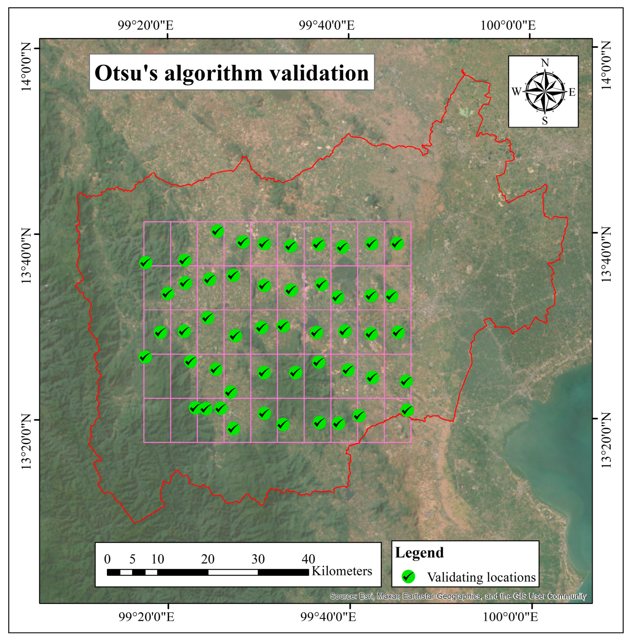
  • We created 50 grids with a point feature at the center of each grid using the Grid Index Features function in ArcGIS 10.8.1 software.
  • We overlaid the grids and points onto Google Earth.
  • We zoomed in on each point, opened the historical satellite data feature, moved the validating point to the nearest large bare land area identifiable through human interpretation, adjusted the image date if necessary, recorded the satellite data acquisition date, and saved the point location.
  • We repeated the process for all 50 points. Figure 5 illustrates the validation locations used for verifying the accuracy of the Otsu algorithm.
  • We exported the points’ locations back to the ArcGIS 10.8.1 software.
  • WE compared each bare land location with the bare land layers at the corresponding or nearest date. We calculated the average deviation in days to quantify the accuracy.
  • We reported the error metrics, including precision, recall, and the average deviation in days.
The confusion matrix (Figure 6) illustrates the performance of the Otsu algorithm in classifying bare land validation points. Out of 50 points, 47 were correctly classified as bare land, yielding an accuracy of 94%. The matrix shows no false negatives, meaning all actual bare land points were identified, resulting in a recall of 100%. Precision, or the accuracy of positive predictions, was also 94%, indicating that most points classified as bare land were indeed bare land. The F1 score, the harmonic mean of precision and recall, further confirms this with a value of approximately 0.969. This supports the robustness and reliability of the algorithm for cassava age estimation, making it a valuable tool for precision agriculture. Table 2 compares the acquisition dates of high-resolution images from Google Earth, used to verify bare land states, with the dates of the bare land layer results from Otsu’s algorithm. The average difference between the dates, which indicates the precision of the validation, is 8.78 days. This level of precision is acceptable because a week causes less significant spectral differences in cassava growth.

3.2. Bare Land Referenced Layer of the Study Area

Based on the methodologies detailed previously, the results of this study have facilitated the creation of a database capable of determining land cover age, not only for cassava but also for various agricultural contexts that require precise age estimation. As demonstrated in Figure 7, this database enhances land management practices by enabling accurate age estimation across different agricultural areas. It should be noted that the pixels classified in the bare land stage might also include built-up areas, water bodies, and low-vegetation areas. Nevertheless, this broad classification does not impact the accuracy of the age layer. To ensure the specificity of the cassava age determination, a highly accurate cassava map provided by the government was utilized to isolate cassava areas for precise age calculations. This selective approach ensures that age estimations are based on the most reliable data available.

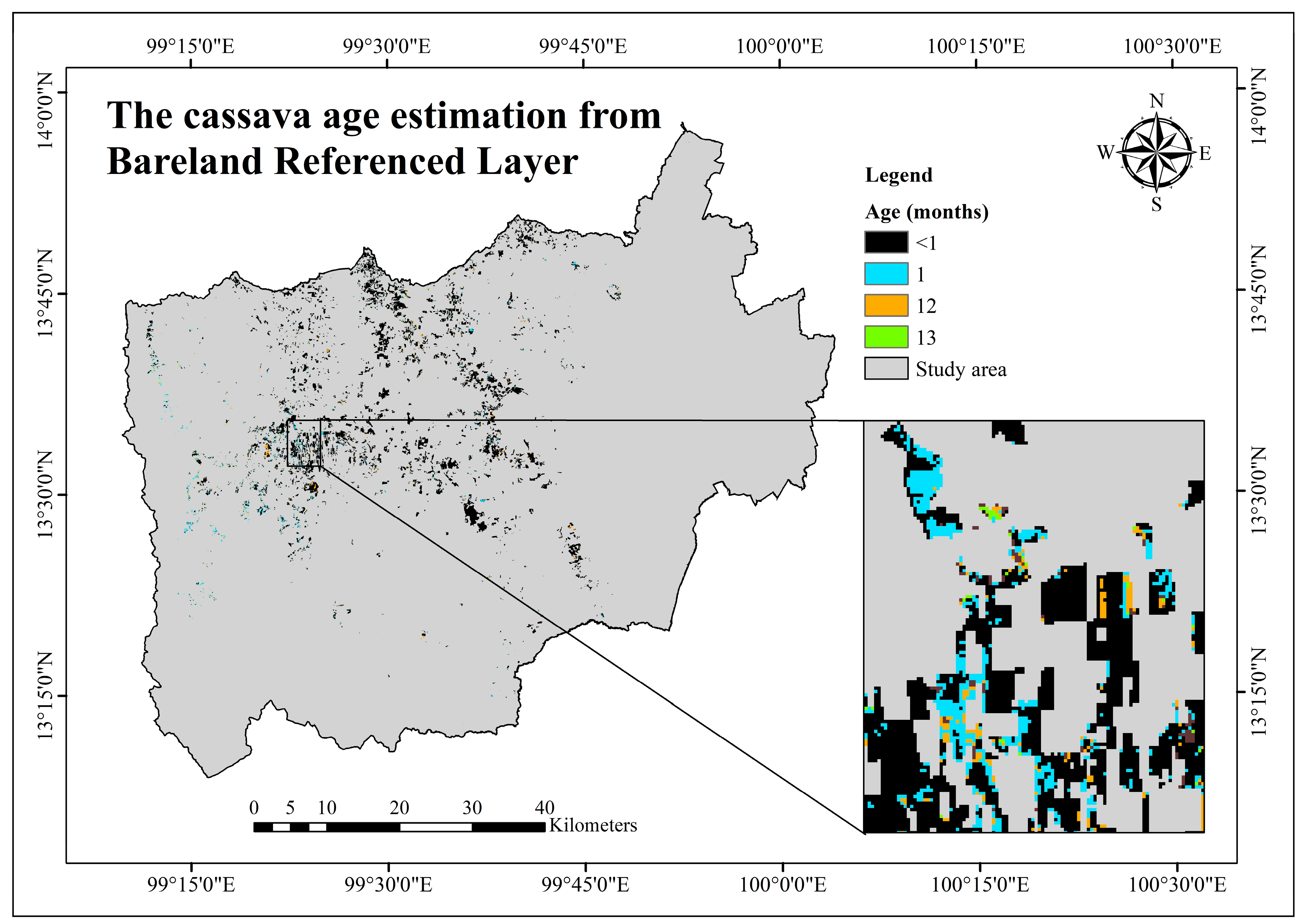
3.3. Cassava Age Estimation Based on the Bare Land Referenced Layers in Ratchaburi, Thailand

The cassava age estimation based on the bare land referenced layers was shown in Figure 8. The age map showcases areas with varying ages of cassava crops, highlighting the crop’s lifecycle stages in alignment with typical agricultural practices in Thailand. Notably, the map identifies fields with lower ages, from 1 month downwards, indicating areas with recently planted or young cassava fields. These correspond well with the typical planting season in Thailand, which begins around April to June, leveraging the rainy season for optimal crop growth. Conversely, the age map also marks fields with higher ages, specifically 12 and 13 months, suggesting these fields have not yet been harvested. This observation is particularly relevant as it reflects fields that may be approaching or exceeding the typical harvest time of 9 to 12 months post-planting, which generally concludes by February. The presence of cassava fields older than 12 months could indicate delays in harvesting due to various factors, such as extended growth periods, weather conditions, or variations in local farming practices.
To further validate the accuracy of the BRAH algorithm’s cassava age estimation, a comprehensive accuracy assessment was conducted using statistical measures and visual inspection.

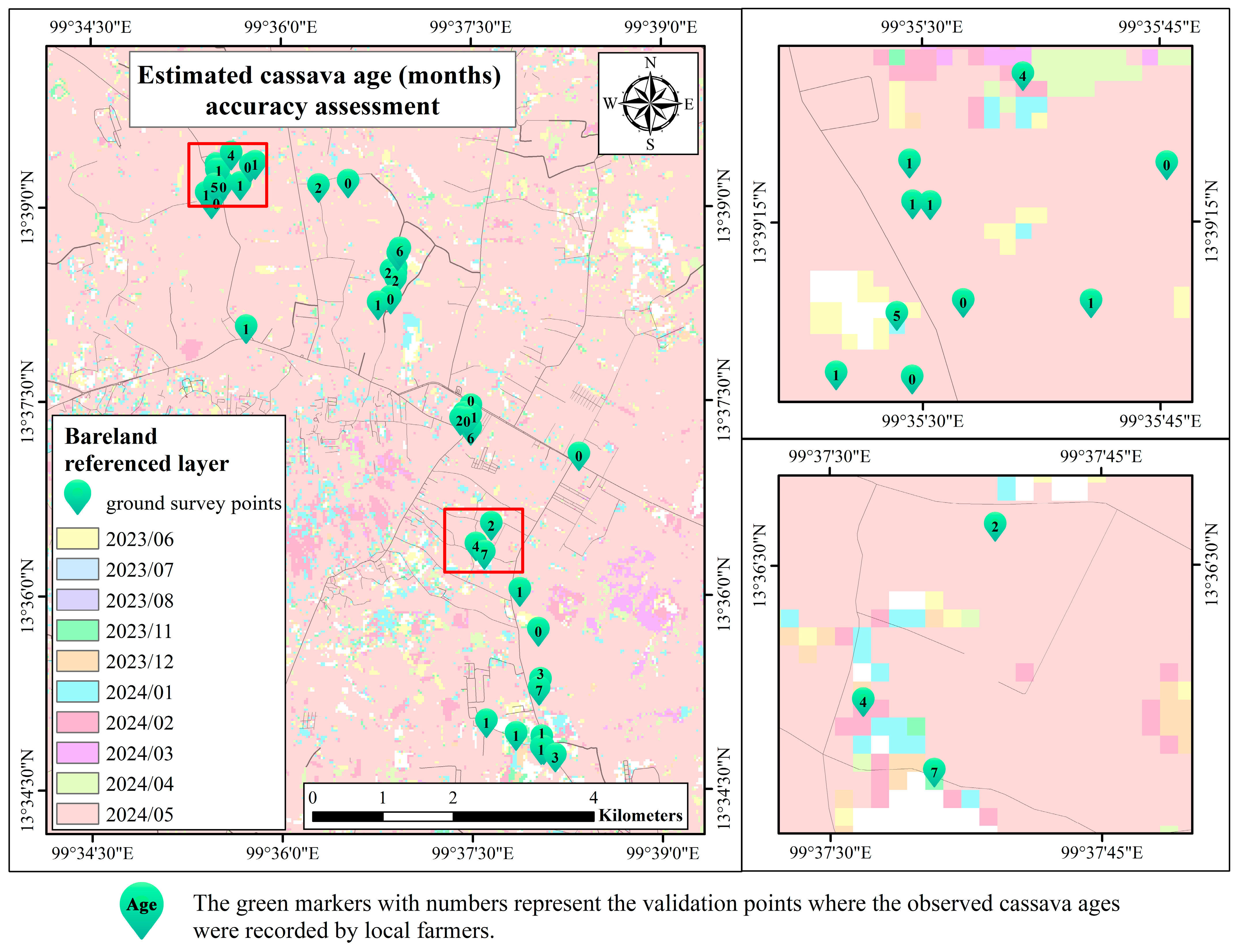
3.3.1. Quantitative Accuracy Assessment

The accuracy of the BRAH algorithm in estimating cassava age was assessed using several statistical measures, comparing predicted cassava ages against observed data from 43 ground survey points recorded by local farmers (data acquisition date: 18 June 2024). The results of this assessment are illustrated in Figure 9.
The mean absolute error (MAE) was found to be 0.349 months, approximately 1.5 weeks. This indicates that, on average, the algorithm’s predictions deviate from the observed ages by a small margin, demonstrating a high level of accuracy. The root mean squared error (RMSE) was calculated to be 0.591 months, or roughly 2.6 weeks, reflecting the typical magnitude of prediction errors and underscoring the algorithm’s precision. The mean bias error (MBE) was determined to be 0.070 months, or approximately 0.3 weeks, indicating a slight overestimation tendency. Additionally, the Pearson correlation coefficient, a measure of the linear relationship between observed and predicted ages, was 0.954, signifying a very strong positive correlation and demonstrating the algorithm’s effectiveness.

3.3.2. Visual Comparison

A visual representation of the validation process is provided in Figure 10 and Table 3, illustrating the spatial distribution of validation points and estimated cassava ages across the study area. Green markers denote the locations of the ground survey points, with the numbers inside these markers indicating the observed cassava ages in months. The background colors represent the estimated cassava ages produced by the BRAH algorithm, with a color legend delineating specific months from June 2023 to April 2024. Land use areas inside the regions should show zero months for specific times.
It is noteworthy that there might be multiple images for each month, providing additional data points and enhancing the robustness of the estimates. Conversely, some months are absent due to the exclusion of images with high cloud contamination, ensuring the integrity of the results by utilizing only high-quality data. Three detailed sections offer zoomed-in views of areas with multiple validation points, allowing for precise examination of the concordance between observed and estimated ages.
The quantitative metrics and visual representation collectively affirm the reliability of the BRAH algorithm in estimating cassava age. The alignment between observed ages (green markers) and estimated ages (background colors) is particularly evident in the zoomed-in sections, validating the algorithm’s predictive accuracy.
The Landsat data, with its 16-day revisiting period, are instrumental in achieving these results. This temporal resolution, approximately every two weeks, ensures frequent capture of crop growth changes, which is crucial for reliable age estimation. The RMSE value of 0.590 months (approximately 2.6 weeks) aligns well with this revisiting period, emphasizing the significance of consistent data acquisition. The presence of multiple images per month strengthens the estimates by averaging out anomalies, while the exclusion of cloud-contaminated months ensures the use of high-quality data. These practices collectively contribute to the robustness and accuracy of the BRAH algorithm’s predictions.
This detailed age mapping provides valuable insights into the temporal dynamics of cassava cultivation across different regions, offering a practical tool for agricultural management and planning. It enables farmers and agricultural advisors to identify and address fields that are due for harvesting, potentially optimizing yield and timing for market sales. Furthermore, these maps can inform broader agricultural strategies by coordinating planting and harvesting schedules across multiple farms, reducing market glut, and stabilizing prices. The insights gained can guide resource allocation, ensuring effective use of irrigation and fertilization at the most beneficial times for crop development.
Moreover, precise age mapping facilitates early intervention for pest and disease management by identifying exact growth stages of cassava fields. This enables timely pest control measures and disease management practices, minimizing crop losses and enhancing overall productivity.

4. Discussion

4.1. Otsu’s Algorithm for Automatic Bare Land Classification of Massive Satellite Data

The enhanced BRAH algorithm, which integrates the BRAH algorithm with the Otsu method, offers a significant advancement in land cover and age estimation by combining temporal data analysis with precise segmentation. Compared to the methods discussed, the enhanced BRAH algorithm stands out for its versatility and high accuracy across different land cover types. Unlike [5,9], which focus on specific crops using moderate-resolution imagery, the Enhanced BRAH algorithm can be applied to various crops and land covers with high-resolution input data, enhancing its applicability in diverse agricultural and ecological contexts.
However, similar to the approach by [8], the enhanced BRAH algorithm requires substantial computational resources and high-quality input data, presenting a potential barrier to widespread implementation. In contrast, the methods by [6,7] utilize more traditional modeling techniques that are less computationally intensive and can be implemented with lower-resolution data. Despite these challenges, the enhanced BRAH algorithm’s ability to deliver precise segmentation and accurate age estimation makes it a powerful tool for remote sensing applications, particularly when computational resources and high-quality data are available.
The application of Otsu’s algorithm for automatic bare land classification marks a significant advancement in handling large satellite image datasets. This study utilized the algorithm across 604 satellite images, highlighting the extensive scope and complexity of the data. Traditional bare land classification methods often depend on manually set NDVI thresholds or require extensive training data for accurate definition, making them time-consuming and impractical for large datasets. Otsu’s algorithm provides a robust alternative by automating the thresholding process. It calculates the optimal threshold that minimizes the intra-class variance between black and white pixels, effectively distinguishing between bare land and vegetated areas. This automation is particularly beneficial for extensive datasets, as it negates the need for manual threshold adjustments or extensive training sets, which are both resource-intensive and slow.
To improve Otsu’s algorithm’s effectiveness in differentiating between bare land and vegetation, histogram equalization was integrated into the preprocessing steps. This technique enhances image contrast, sharpening the distinction between bare land and vegetation. By adjusting the image contrast, histogram equalization reduces the spectral value differences between bare land and vegetation, aiding Otsu’s algorithm in more accurately and effectively classifying the images. The combination of Otsu’s algorithm and histogram equalization has proven to be an effective tool for processing and analyzing satellite imagery. Our combined approach not only accelerates the classification process but also boosts the accuracy and reliability of the results. By automating segmentation and enhancing contrast, this method addresses significant challenges associated with conventional NDVI-based classification techniques, offering a scalable and adaptable solution for various geographic and environmental settings.
Alternatively, advanced machine learning algorithms, like random forest (RF), can also be effectively used for bare land classification. The transferable random forest model is particularly interesting as it can be trained once and applied across the entire dataset. However, preparing the training data for RF is a challenging task and requires extensive ground truth data, which can be resource-intensive. While RF provides a sustainable approach for future applications, our current choice of Otsu’s method is due to its lack of requirement for training data. This feature makes our BRAH algorithm fully automatic and fast to process, which is advantageous for handling large datasets without the need for extensive ground truth data.

4.2. Limitations and Suggestions

4.2.1. Data Quality

The classification of bare land within the dataset is significantly influenced by floating matter, such as haze, which alters the reflectivity seen in satellite imagery, thereby affecting accuracy. This was particularly noted during the analysis phases where the reflectivity characteristics varied, impacting the classification results. To address this issue, the quality assurance (QA) band was utilized to filter out affected pixels, enhancing the reliability of the classification outcomes. This strategic use of the QA band helps in identifying and excluding pixels impacted by atmospheric conditions, like haze, ensuring that only data with high confidence in their reflectivity characteristics are used for analysis. However, it is important to exercise caution when using the quality assurance (QA) band, particularly because the interpretation of QA flags requires careful consideration. For instance, while the QA band can effectively filter out pixels affected by clouds, haze, or shadows, it may also inadvertently exclude some viable data if the thresholds are not set or interpreted correctly. This could lead to a reduction in the usable data, potentially affecting the classification outcomes or the representativeness of the analysis. Additionally, the QA bands contain a range of information, from basic cloud cover to more complex attributes, like aerosol levels or land/water distinctions, which can complicate data processing. Misinterpretation of these bands can lead to errors in masking or classifying data, particularly in diverse ecological or meteorological conditions.

4.2.2. NDVI Thresholding

While the original study set NDVI thresholds between 0 and 0.2 based on limited ground data [2], in this article, the Otsu method was employed due to several critical factors. Firstly, manual verification of NDVI thresholds for each image is impractical given the extensive number of images and the absence of comprehensive ground truth data for certain periods. Secondly, manually setting thresholds is a time-consuming task that can introduce subjectivity and inconsistency, especially when dealing with large datasets spanning diverse environmental conditions. The Otsu method offers a systematic, automated approach that efficiently determines optimal thresholds, enhancing the scalability and reliability of bare land classification across the dataset.
However, it is important to note that the NDVI values used in this study were processed using histogram equalization to enhance contrast. This processing step alters the original NDVI values, and the thresholds determined by the Otsu method are specific to these adjusted values. As such, we did not extract and record the specific NDVI thresholds during the algorithm’s execution, as they are unique to each image and not directly comparable across the dataset. Therefore, plotting a chart with image dates and NDVI thresholds would not provide meaningful or comparable information.

4.2.3. Temporal Resolution of the Dataset

The temporal resolution of the satellite data used in the original study was noted as a limitation, particularly in rapidly changing landscapes, such as agricultural fields with short growing cycles. The low temporal resolution of the satellite data may lead to missing crucial stages, like the bare land phase, which is essential for accurate land cover analysis. This can result in inaccuracies within the bare land referenced layer, potentially affecting the overall reliability of the study outcomes.
Although the monthly resolution of the satellite data was deemed sufficient for tracking the growth stages of cassava, which typically has a harvest cycle of about 9 to 12 months, there is room for improvement. To enhance the accuracy of age determination for cassava, it is recommended to utilize satellite data with a much higher revisiting frequency. Satellite systems with a higher temporal resolution can provide more frequent observations, thereby capturing rapid changes in land cover more effectively and reducing the risk of missing critical transitions.
To address these challenges, future research should focus on employing satellite data with higher temporal resolutions and extending the dataset to include older imagery. This approach would provide a more comprehensive understanding of land cover dynamics and improve the accuracy of age estimations for cassava and other similarly short-cycle crops.

5. Conclusions

The application of the BRAH algorithm, refined with Otsu’s automated thresholding, represents a significant advancement in precision agriculture, particularly in the context of large-scale satellite data analysis. This study demonstrated the algorithm’s ability to accurately classify bare land and estimate crop age, with a specific focus on cassava cultivation in Thailand. The integration of histogram equalization improved the distinction between bare land and vegetated areas, enhancing the overall effectiveness of the age estimation process. The results confirmed the method’s alignment with actual agricultural timelines, supporting its potential for broader application in agricultural management. Despite challenges, such as data availability and the need for higher temporal resolution in satellite imagery, this approach marks a substantial improvement over traditional methods, offering a scalable and reliable solution for future agricultural planning and sustainability efforts.
Future research should aim to incorporate satellite data with higher revisiting frequencies, such as data from the Sentinel-2 mission, which provides a five-day revisit time, to capture rapid changes in crop conditions. Additionally, the use of unmanned aerial vehicles (UAVs) equipped with multispectral and hyperspectral sensors can provide high-resolution, real-time data for more precise monitoring and analysis. Emphasizing unsupervised methods, such as clustering techniques (e.g., k-means, DBSCAN) and anomaly detection algorithms, will help in reducing human intervention and automating the process further. Extending the dataset to include older historical aerial imagery, combined with advanced image processing techniques, like deep learning-based super-resolution, can facilitate long-term land cover analysis. Incorporating these technologies will further refine the algorithm and broaden its applicability in various agricultural contexts.
While other algorithms can be explored for the bare land classification task, the BRAH algorithm provides a robust workflow that can integrate with these advancements to achieve more accurate and reliable age estimation in a fully automated manner.

Author Contributions

Conceptualization, S.B.; methodology, S.B.; software, S.B.; validation, S.B.; formal analysis, S.B. and T.S.; investigation, N.P.; resources, N.P.; data curation, S.B.; writing—original draft preparation, S.B., T.S. and N.P.; writing—review and editing, S.B.; visualization, S.B.; supervision, S.B. and T.S.; funding acquisition, T.S. and N.P. All authors have read and agreed to the published version of the manuscript.

Funding

This research was funded by the Faculty of Social Sciences, Kasetsart University, grant year 2024, and the Faculty of Environment, Kasetsart University, grant year 2024.

Data Availability Statement

The primary raw data used in this study are accessible on EarthExplorer, available at https://earthexplorer.usgs.gov/ (accessed on 26 April 2024). Secondary data are not available for distribution. However, data derived from this study that support the findings are available upon request from the corresponding author.

Acknowledgments

The authors would like to thank the anonymous reviewers for their constructive and valuable suggestions on the earlier drafts of this manuscript.

Conflicts of Interest

The authors declare no conflicts of interest.

References

  1. International Society of Precision Agriculture (ISPA). Definition of Precision Agriculture. Available online: https://www.ispag.org/about/definition (accessed on 23 June 2024).
  2. Boonprong, S.; Khantachawana, A. Bare Land Referenced Algorithm from Hyper-Temporal Data (BRAH) for Land Use and Land Cover Age Estimation. Land 2023, 12, 1387. [Google Scholar] [CrossRef]
  3. Ghannam, N. Precision Farming Enables Climate-Smart Agribusiness. EMCompass 2021, 46, 121268. Available online: http://documents.worldbank.org/curated/en/387381510726761684/Precision-farming-enables-climate-smart-agribusiness (accessed on 6 May 2024).
  4. Fang, S.; Xuerong, S.; Mengyu, L.; GiHoon, H. Enhanced Ocean Carbon Sinks Triggered by Climate Change Seen from the Space. 2022. Available online: https://unfccc.int/sites/default/files/resource/IMBeR%20OCPC%20Poster%20for%20FE%40COP%2027.pdf (accessed on 6 April 2024).
  5. Chumkesornkulkij, K.; Kasetkasem, T.; Rakwatin, P.; Eiumnoh, A.; Kumazawa, I.; Buddhaboon, C. Estimated rice cultivation date using an extended Kalman filter on MODIS NDVI time-series data. In Proceedings of the 2013 10th International Conference on Electrical Engineering/Electronics, Computer, Telecommunications and Information Technology (ECTI-CON), Krabi, Thailand, 15–17 May 2013; IEEE: New York, NY, USA, 2013; pp. 1–6. [Google Scholar] [CrossRef]
  6. Chen, G.; Thill, J.-C.; Anantsuksomsri, S.; Tontisirin, N.; Tao, R. Stand age estimation of rubber (Hevea brasiliensis) plantations using an integrated pixel- and object-based tree growth model and annual Landsat time series. ISPRS J. Photogramm. Remote Sens. 2018, 144, 94–104. [Google Scholar] [CrossRef]
  7. Baker, P.J. Tree age estimation for the tropics: A test from the Southern Appalachians. Ecol. Appl. 2003, 13, 1718–1732. [Google Scholar] [CrossRef]
  8. Agustin, S.; Tjandrasa, H.; Ginardi, R.V.H. Deep Learning-based Method for Multi-Class Classification of Oil Palm Planted Area on Plant Ages Using Ikonos Panchromatic Imagery. Int. J. Adv. Sci. Eng. Inf. Technol. 2020, 10, 2200. [Google Scholar] [CrossRef]
  9. Madugundu, R.; Al-Gaadi, K.A.; Tola, E.; Edrris, M.K.; Edrees, H.F.; Alameen, A.A. Optimal Timing of Carrot Crop Monitoring and Yield Assessment Using Sentinel-2 Images: A Machine-Learning Approach. Appl. Sci. 2024, 14, 3636. [Google Scholar] [CrossRef]
  10. Tom, A.; Orawan, S.; Yelto, Z. Cassava Production and Processing in Thailand. 2018. Available online: http://www.agribenchmark.org/fileadmin/Dateiablage/B-Cash-Crop/Reports/CassavaReportFinal-181030.pdf (accessed on 6 April 2024).
  11. Food and Agriculture Organization of the United Nations. Save and Grow: Cassava—A Guide to Sustainable Production Intensification. 2013. Available online: https://openknowledge.fao.org/items/0d0333b5-c005-46a5-8594-bdd5caa3856d (accessed on 6 April 2024).
  12. Manganyi, B.; Lubinga, M.H.; Zondo, B.; Tempia, N. Factors Influencing Cassava Sales and Income Generation among Cassava Producers in South Africa. Sustainability 2023, 15, 14366. [Google Scholar] [CrossRef]
  13. Han, S.-H.; Mutahira, H.; Jang, H.-S. Prediction of Sensor Data in a Greenhouse for Cultivation of Paprika Plants Using a Stacking Ensemble for Smart Farms. Appl. Sci. 2023, 13, 10464. [Google Scholar] [CrossRef]
  14. Onyeneke, C.J.; Umeh, G.N.; Onyeneke, R.U. Impact of Climate Information Services on Crop Yield in Ebonyi State Nigeria. Climate 2023, 11, 7. [Google Scholar] [CrossRef]
  15. Olarinde, L.O.; Abass, A.B.; Abdoulaye, T.; Adepoju, A.A.; Fanifosi, E.G.; Adio, M.O.; Adeniyi, O.A.; Wasiu, A. Estimating Multidimensional Poverty among Cassava Producers in Nigeria: Patterns and Socioeconomic Determinants. Sustainability 2020, 12, 5366. [Google Scholar] [CrossRef]
  16. US Geological Survey. Landsat Collection 2 Level 2 Science Products. Available online: https://www.usgs.gov/landsat-missions/landsat-collection-2-level-2-science-products (accessed on 28 January 2024).
  17. Guo, Y.; Wang, Y.; Meng, K.; Zhu, Z. Otsu Multi-Threshold Image Segmentation Based on Adaptive Double-Mutation Differential Evolution. Biomimetics 2023, 8, 418. [Google Scholar] [CrossRef] [PubMed]
  18. Liu, Y.; Gu, G.; Chen, Q. Optimized Contrast Enhancement for Infrared Images Based on Global and Local Histogram Specification. Remote Sens. 2019, 11, 849. [Google Scholar] [CrossRef]
Figure 1. The area of cassava cultivation in Ratchaburi Province, Thailand. The map shows the distribution of cassava fields within the province, highlighting the concentration of cultivation areas. An inset map of Thailand indicates the location of Ratchaburi Province within the country.
Agriculture 14 01075 g001
Figure 2. Distribution of acquisition dates of satellite images.
Agriculture 14 01075 g002
Figure 3. The enhanced BRAH algorithm used in this study.
Agriculture 14 01075 g003
Figure 4. (A) The example of NDVI layer and (B) the example bare land layer from Otsu’s algorithm.
Agriculture 14 01075 g004
Figure 5. Validation of Otsu’s algorithm in Ratchaburi Province.
Agriculture 14 01075 g005
Figure 6. Confusion matrix for the validation of Otsu’s algorithm.
Agriculture 14 01075 g006
Figure 7. Bare land referenced layer derived from 604 satellite images (last data update: 1 April 2024). The legends on the map display dates only from the years 2023 and 2024. It is important to note that the resolution of the bare land referenced layer, which spans from 1987 to 2024, is consistent with the resolution indicated by the map legends.
Agriculture 14 01075 g007
Figure 8. The cassava age estimation map. Please note that this map was created with the assumption that the input cassava area map was generated on 1 May 2024. However, the actual date of the official cassava area map typically corresponds to the end of the year, as it is provided annually. This assumption is considered not critically significant, as the cassava area is unlikely to undergo substantial changes within such a short interval.
Agriculture 14 01075 g008
Figure 9. Quantitative accuracy assessment of cassava age estimation using the BRAH algorithm. The assessment is based on 43 ground survey samples. The results revealed a mean absolute error (MAE) of 0.349, a root mean squared error (RMSE) of 0.591, a mean bias error (MBE) of 0.0698, and a Pearson correlation coefficient of 0.9536.
Agriculture 14 01075 g009
Figure 10. Visual accuracy assessment of cassava age estimation, showing observed ages at validation points. Land use areas inside the regions should show zero months for the specific times (last data update: 20 May 2024).
Agriculture 14 01075 g010
Table 1. Overview of satellite data utilized in this study.
SensorsPath/RowQuantities
Landsat 4 Thematic Mapper (TM)129/0512
Landsat 5 Thematic Mapper (TM)130/051127
129/051122
Landsat 7 Enhanced Thematic Mapper (ETM+)129/05115
130/05022
130/05117
Landsat 8 Operational Land Imager (OLI)129/05174
130/05081
130/05184
Landsat 9 Operational Land Imager (OLI)129/05120
130/05024
130/05116
Total604
Table 2. Comparison of the acquisition dates of high-resolution images from Google Earth, used to verify bare land states, with the dates of the bare land layer results from Otsu’s algorithm. IDs indicate the validating locations in Figure 5, arranged from left to right and top to bottom. The misclassification locations were highlighted in bold letters.
IDsBR Layer
Output Date
Validated *
Bare Land Stage Date
TradeoffIDsBR Layer
Output Date
Validated *
Bare Land Stage Date
Tradeoff
111-May-20213-May-202182617-Jan-202111-Jan-20216
219-Apr-202315-Apr-202342717-Jan-202111-Jan-20216
38-Feb-20197-Feb-20191285-Feb-202112-Feb-20217
48-Feb-20197-Feb-20191295-Feb-202112-Feb-20217
517-Jan-202111-Jan-20216305-Feb-202112-Feb-20217
617-Jan-202111-Jan-20216316-Sep-202225-Jul-202243
717-Jan-202111-Jan-202163212-May-20213-May-20219
85-Feb-202112-Feb-202173312-May-20213-May-20219
95-Feb-202112-Feb-202173412-May-20213-May-20219
105-Feb-202112-Feb-202173517-Jan-202111-Jan-20216
1119-Apr-202315-Apr-202343617-Jan-202111-Jan-20216
122-Mar-201911-Mar-201993717-Jan-202111-Jan-20216
131-Jan-20197-Feb-2019373824-Feb-202128-Feb-20214
141-Jan-20197-Feb-2019373924-Feb-202128-Feb-20214
1517-Jan-202111-Jan-202164023-Jan-202111-Jan-202112
1617-Jan-202111-Jan-20216415-Nov-20183-Nov-20182
1717-Jan-202111-Jan-20216425-Nov-20183-Nov-20182
1817-Jan-202111-Jan-202164312-May-20213-May-20219
1916-Jan-202214-Jan-202224412-May-20213-May-20219
205-Feb-20215-Feb-202104527-Jun-202225-Jul-202228
2119-Apr-202315-Apr-202344627-Jun-202225-Jul-202228
2219-Apr-202315-Apr-202344724-Feb-202128-Feb-20214
2312-May-20213-May-202194824-Feb-202128-Feb-20214
2412-May-20213-May-20219495-Feb-202112-Feb-20217
2517-Jan-202111-Jan-20216505-Feb-202112-Feb-20217
Average7.92 Average9.64
Grand average8.78
* The validated bare land stage dates are based on the availability of high-resolution image provided from Google Earth.
Table 3. Comparison of observed and predicted cassava ages (in months) using the BRAH algorithm. The table shows the observed and predicted ages for 43 ground survey samples. Most errors occurred at the ages of 0 and 1 months because the algorithm tends to overestimate or underestimate very young cassava plants, likely due to their minimal distinguishable features in satellite imagery.
No.Observed Age
(Month)
Predicted Age
(Month)
No.Observed Age
(Month)
Predicted Age
(Month)
No.Observed Age
(Month)
Predicted Age
(Month)
11115212911
21116013021
31117013111
40118663233
50119213311
61120113411
71121213555
81122213601
90123443711
100124773844
115525113911
121126014022
132127334166
141128774211
4301
Disclaimer/Publisher’s Note: The statements, opinions and data contained in all publications are solely those of the individual author(s) and contributor(s) and not of MDPI and/or the editor(s). MDPI and/or the editor(s) disclaim responsibility for any injury to people or property resulting from any ideas, methods, instructions or products referred to in the content.

