Abstract
The solar greenhouse is a significant agricultural facility in China. It enables the cultivation of crops during periods that do not coincide with the natural growing season, thus alleviating the pressure on the supply of fruits and vegetables during the winter months. The primary rationale behind the necessity of greenhouse cultivation lies in the fact that the temperature conditions conducive to optimal crop growth can be precisely replicated within this controlled environment. However, it is important to acknowledge that a distinct low-temperature area persists under the film during the overwintering period, with the precise delineation of its boundaries and distribution patterns remaining uncertain. In order to investigate the characteristics of the temperature distribution within the marginal region under the solar greenhouse film, experimental studies, CFD simulations, and LSTM prediction models were employed. The results of these studies indicate that, during the overwintering period, a low-temperature region was observed with approximately equal temperatures near the film membrane. The maximum horizontal distance from the south-side bottom corner was 6130 mm, while the minimum height from the ground was 600 mm. The lowest temperature in the low-temperature region was 4 °C, and the maximum observed temperature difference within the same period in different months was 1 °C. Additionally, a region of elevated temperatures was observed under the film. The lowest temperature in this region was 36.7 °C, and the highest temperature point was within the optimal range for crop growth. The CFD numerical simulation results were consistent with the actual observations, and the LSTM prediction model demonstrated high reliability. The findings of this study offer a theoretical foundation for the distribution of high and low temperatures in solar greenhouses. Furthermore, the developed prediction model provides the necessary buffer time for control, thus enhancing the efficiency of greenhouse cultivation.
1. Introduction
In 2020, a global population of 264 million individuals faced the challenge of food scarcity [1]. This challenge is projected to worsen in the coming decades due to the onset of global conflicts, climatic extremes, rapid population growth, and the gradual depletion of energy resources [2]. As a modern agricultural production method [3], the use of unique facility structures combined with various technical means can extend the growing season or provide suitable environmental conditions for plant growth [4], improving the quality of agricultural production and increasing income. As the mainstay of facility-based agriculture in China [5], the solar greenhouse can create a suitable microclimate for plants and reduce the carbon dioxide emissions [6]. With an area of 1/3 of the total area of vegetable facilities [7], the solar greenhouse can help to alleviate the mismatch between the supply and demand of agricultural products in the off-season [8] and help to achieve the goal of China’s “dual-carbon” strategy [9]. However, modern solar greenhouse production still faces the challenge of a mismatch between environmental regulation and crop demand [10]. This mismatch between the supply and demand environmental conditions leads to crop yield reduction or death.
The main reason for this problem is that the plant yield is affected by the microclimate of the greenhouse, which includes indoor light [11], temperature and humidity [12], and CO2 concentration [13]. The greenhouse microclimate directly affects the plant metabolic activity, which in turn affects the crop yield [14]. The effects of temperature and humidity on plant growth are particularly pronounced [15]. Controlling the temperature and humidity throughout the greenhouse within the correct range is essential to ensure uniform plant growth [16].
The winter night-time indoor air temperature is an important indicator of the greenhouse insulation performance because changes in the indoor air temperature have a similar trend to changes in the interior surface temperature of a wall, the indoor ground temperature, and the plant body temperature [17]. More importantly, the temperature can alter the enzyme activity, which in turn affects the photosynthetic rate, growth, quality, and morphology of plants [18]. The marginal effects of the temperature environment of solar greenhouses are quite clear, and the marginal zone temperature environments of solar greenhouses are discussed in the literature by many researchers [19]. In the solar greenhouse, there is a marginal film effect in the film area, which is the coldest area in the solar greenhouse at night in winter, and the range of this area is large [20]. However, there are fewer studies on the marginal film effect area in the solar greenhouse [21]. The term “film marginal effect” is used to describe the area inside the solar greenhouse that is closer to the film and experiences equal temperatures.
To investigate the mechanism of greenhouse air temperature change, many scientists have used mathematical models, experimental studies, CFD 19.0 software, and neural network models. Esmaeli et al. [22] developed a greenhouse thermal model by analyzing and calculating the energy balance process of indoor air. Lei et al. [15] developed a one-dimensional transient temperature prediction model for the Chinese Assembled Solar Greenhouse (CASG) based on the energy balance principle. Shamim et al. [23] proposed a model on the sensitivity of heat consumption in solar greenhouses, and the results showed that the main parameters of the air thermal conductivity model affected the model output, and the thermal properties of the cover, insulation, and greenhouse perimeter had greater sensitivity to greenhouse heat loss. Mechanistic models have the advantage of strong interpretability and good extrapolation. However, the problems of difficult access to their parameters and the high degree of variation in the boundary conditions lead to difficulties in applying them for long-term accurate prediction [24].
The existence of an inverse temperature phenomenon was observed in greenhouses of different heights, where the temperature tended to increase and then decrease [25]. In addition, a study on the temperature and humidity of the crop film area in a solar greenhouse showed that there were significant differences in the temperature and humidity under different light conditions [26]. The existing studies [17,27] indicate spatiotemporal variations in the internal temperature of the solar greenhouse. However, regardless of the weather conditions, indoor air temperatures change more drastically along vertical and horizontal directions, while the rate of change along the greenhouse length is more moderate [28].
Many scholars [29,30] have used CFD to study the changes in the thermal environment inside solar greenhouses under different working conditions. Due to the complex structure of a solar greenhouse, the film temperature in particular was affected by various factors such as crop growth, external light, wall heat storage, and cover materials. These factors caused the spatial distribution of the film temperature to become nonlinear and variable, making accurate simulation using CFD methods relatively difficult [31]. Predicting the solar greenhouse temperatures not only provided a basis for the greenhouse environmental management decisions to reduce crop risks but also served as basic research for feedback climate control strategies. Recently, deep learning methods have become a hot topic of research because of their strong nonlinear approximation and deep feature extraction capabilities, which provided good theoretical support for multidimensional time series data [32]. Tana et al. [26] studied the temperature and humidity test data at different locations within a crop’s film, training and optimizing Elman neural networks with test data. Dong et al. [33] used the SOGREEN model to validate the measurement data from Canadian solar greenhouses. The model can predict the environmental parameters of solar greenhouses with reasonable accuracy, but the model needed to be further improved to minimize the prediction error, especially for the north wall. Gong Jianlin et al. [34] analyzed the relationship between outdoor meteorological data and indoor temperature changes and developed an indoor temperature prediction model based on covariance theory to predict the average temperature inside the solar greenhouse. The prediction accuracy was high and significantly better than that of the commonly used traditional linear regression model. Mahmood et al. [35] proposed a greenhouse temperature control method based on a data-driven model using artificial neural networks for the dynamic prediction of indoor temperature; Jung et al. [36] applied three deep learning-based neural network models to predict the changes in the humidity and thermal environment in a greenhouse; Moon et al. [37] used a two-dimensional convolutional neural network to establish the relationship between the indoor microclimate and radiation to estimate the greenhouse temperature environment; Hu Jin et al. [25] proposed a solar greenhouse temperature prediction model based on 1 DCNN-GRU. One or both methods alone were used in the above studies to accurately and efficiently predict the greenhouse growth. However, they were not able to accurately predict the government regulation of crop growth because they ignored crop transpiration and photosynthesis.
In summary, many scholars have studied the internal temperatures of solar greenhouses, but the internal low-temperature region under the solar greenhouse film was still unclear at night, and this part of the region was the lowest-temperature region of the solar greenhouse, which is extremely important for the heat conservation of solar greenhouses. This region of the greenhouse exhibited the lowest temperature, which was of paramount importance for the insulation of the greenhouse. In comparison to the other areas of the greenhouse, the temperature of the region with the smallest difference between the outdoor temperature and the temperature within the greenhouse, thereby reducing the heat loss, indirectly protects the greenhouse from the high temperature of the region of heat loss. Therefore, this paper investigated the marginal effect under the solar greenhouse film by an experimental study, the Python-based learning model, and CFD numerical simulations. This study analyzed the factors influencing the marginal effect of air temperature in solar greenhouses, defined solar greenhouses to determine the marginal effect area under the screen, and provided theoretical and data support for greenhouse cultivation and the greenhouse heating area.
In recent years, solar greenhouses have been widely adopted in agricultural production worldwide due to their energy efficiency and ability to extend growing seasons. However, one of the major challenges faced by solar greenhouse operations is the uneven temperature distribution within the structure, which can significantly impact the crop yield and quality. Among the various regions within a greenhouse, the cryogenic region, which exhibits the lowest temperatures, is critically important for the overall insulation performance. This study is concerned with the understanding and optimization of the temperature distribution in the cryogenic region of solar greenhouses. By conducting comprehensive temperature analyses and comparing different greenhouse areas, the aim is to identify the key factors contributing to heat loss and to propose effective insulation strategies. The primary contribution of this research lies in its detailed investigation of the cryogenic region’s thermal characteristics and its practical recommendations for improving greenhouse insulation. The findings of this study provide valuable insights that can inform the design and operation of more efficient solar greenhouses, thereby enhancing agricultural productivity and sustainability. This work not only fills a gap in the current literature but also offers a foundation for future studies aiming to optimize greenhouse environments under varying climatic conditions.
2. Materials and Methods
2.1. Experimental Greenhouse
The solar greenhouse has the capacity to sustain a comfortable internal temperature at night during the winter months and to absorb heat from the surrounding environment during the day, by stowing away and subsequently unstowing the quilts. The solar greenhouse may be controlled with respect to ventilation and heat dissipation by adjustment of the upper and lower air outlets throughout the year.
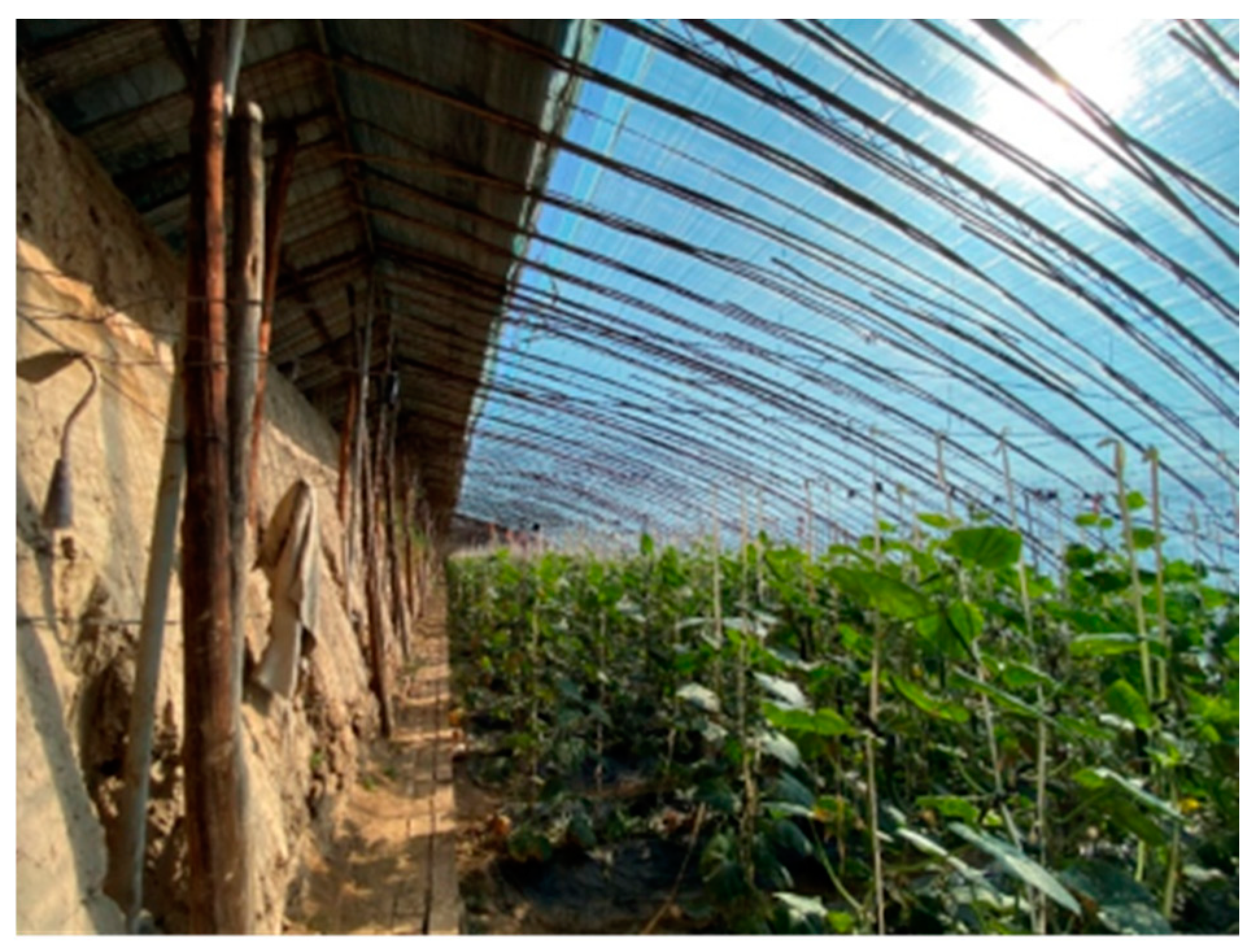
The experimental greenhouse (Figure 1) is a passive solar greenhouse, whereby the medium acts as a storage unit for solar energy, subsequently releasing this stored energy to the interior of the greenhouse. The experimental greenhouse is situated in Taigu, Shanxi, China. The greenhouse, oriented north to south, is 75 m long and has a span of 10 m, with a ridge height of 4.3 m. The east and west walls are 3 m long and the north wall is an Aboriginal wall that is 8 m wide at the base and 2 m wide at the top. The main skeleton is composed of 28 elliptical steel tubes with a skeletal spacing of 2.8 m, and the top of the north wall is constructed using about 2 m-long wooden sticks affixed to the skeleton, covered with a polythene (PO) film. The structural dimension section of the selected greenhouse is depicted in Figure 2.

Figure 1.
Test greenhouse.
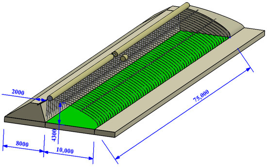
Figure 2.
Structural dimensions section.
The experimental greenhouse was planted with cucumbers, which were cultivated under raised beds and drip irrigation. The walkway width on the north side was 67 cm, and the crop rows were spaced approximately 45 cm apart, with 10 cm spacing between the crops. The nearest distance between the inner crop and the southern architrave was 600 mm.
2.2. Testing Methods and Materials
2.2.1. Test Materials
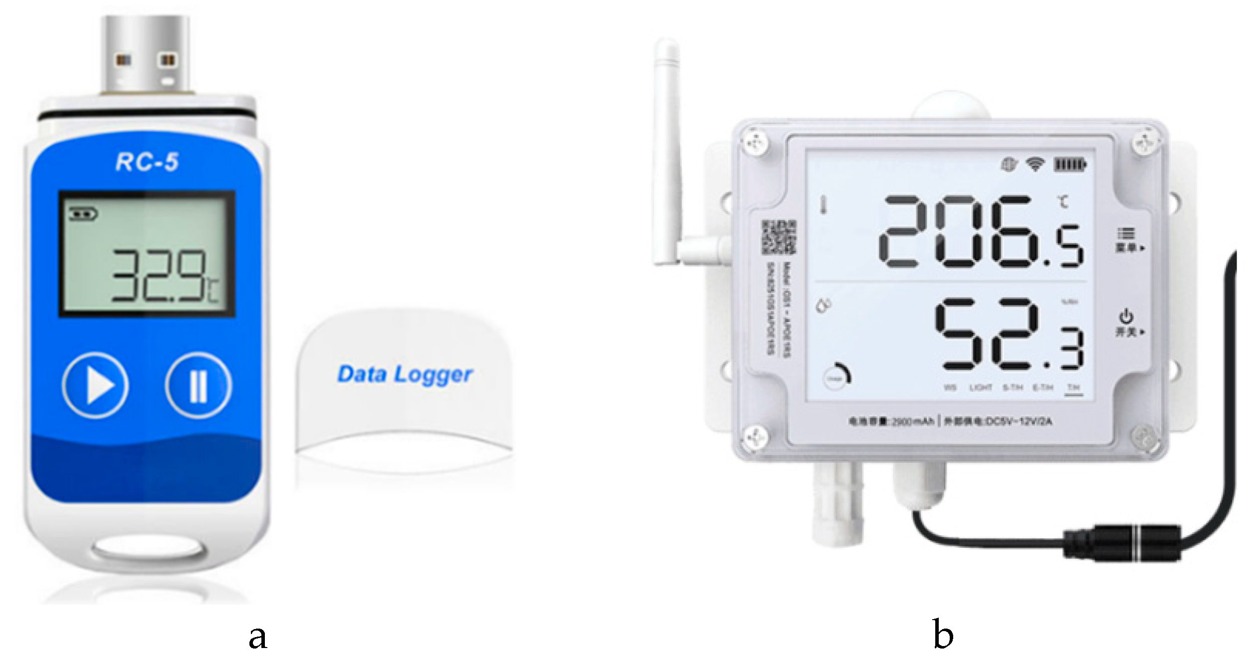
The temperature of indoor and outdoor air was monitored using the RC-5 U-disk temperature recorder, as illustrated in Figure 3a. This device incorporates a built-in NTC thermistor, manufactured by Jingchuang Electric Co in Jiangsu, China. The device’s dimensions were 80 mm long, 33 mm wide, and 14 mm high. It was equipped with a built-in wide-temperature lithium battery, which enabled continuous operation for approximately three months. The temperature measurement range of the equipment was −30 °C~ +70 °C, in the temperature measurement range of −20 °C~ +40 °C, and the measurement accuracy was ±0.5 °C; the rest was ±1 °C. The recording interval should be set to 6 min. This enabled the storage of 32,000 sets of data, which was the maximum capacity of the storage unit in question.

Figure 3.
Testingequipment.
Indoor light and carbon dioxide measurements were conducted using GS1 industrial-grade loggers, as depicted in Figure 3b. The device was designed to be fully enclosed and waterproof, dustproof, pressure-resistant, and capable of operating at high temperatures, equipped with a 2900 mAh lithium battery, and a power-saving mode. The device is equipped with integrated temperature, humidity, and light sensors, in addition to an external CO2 sensor. The temperature range was −20 to 60 °C with an accuracy of ±2 °C; the humidity range was 10 to 90% with an accuracy of ±2 %RH. The light range was 0.01 to 157,000 Lux with an accuracy of ±10%. The internal memory chip was capable of caching 300,000 data points. CO2 measurement range was 0 to 40,000 ppm.
2.2.2. Test Method
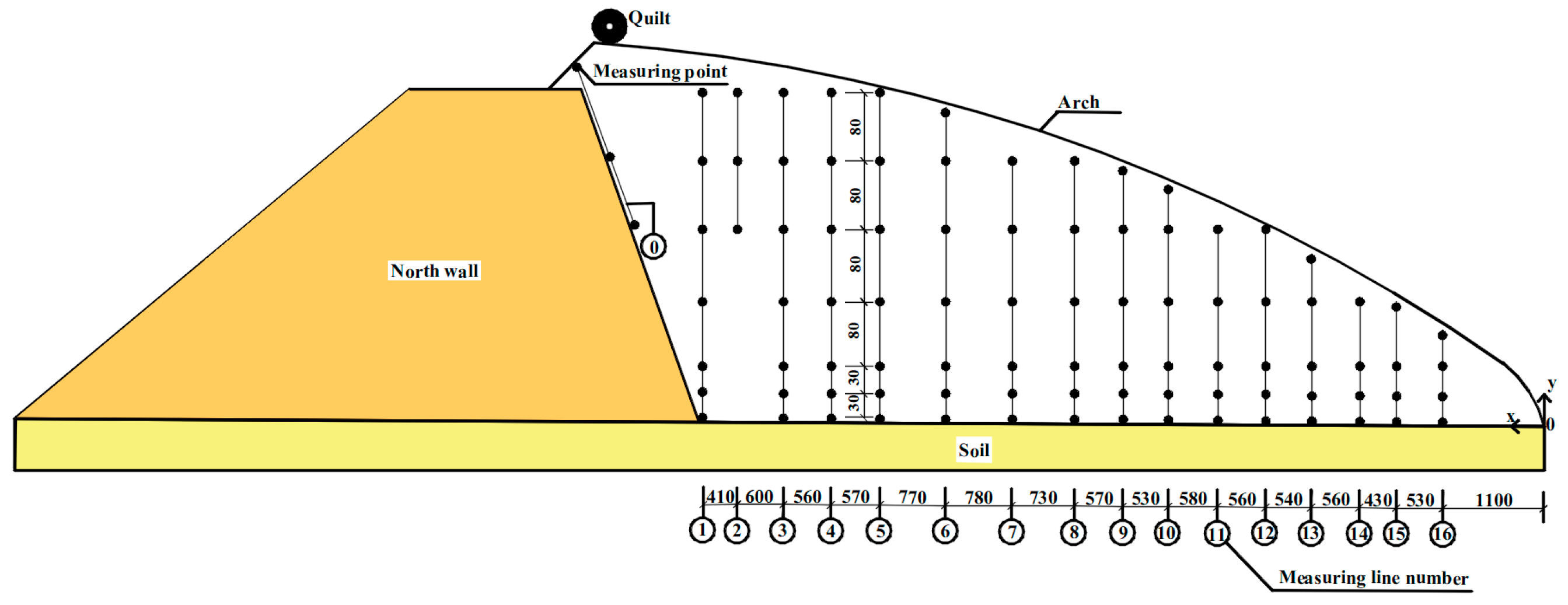
A cross-section was selected for the purpose of arranging the sensors at the midpoint in the east–west direction. The test period commenced on 24 September 2023 and concluded on 7April 2024. In order to ascertain the optimal configuration of pulleys for hanging temperature sensors, a series of 16 positions were selected in the middle cross-section of the greenhouse along a north–south direction. These positions were used to install pulleys at different heights, resulting in a total of 16 lines and 94 temperature sensors (RC-5). The greenhouse internal layout of each line is illustrated in Figure 4.
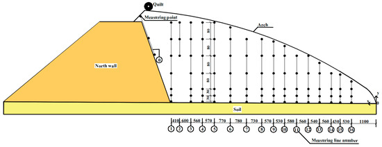
Figure 4.
Layout of measurement lines.
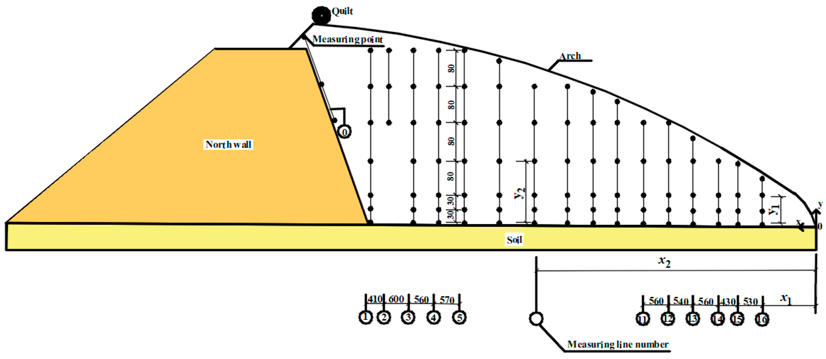
The location of the temperature measurement points was as follows: the south foot of the cross-section in the span was taken as the coordinate origin. The value upward was taken as the y-axis and northward as the x-axis, and a coordinate system was established.
The route from north to south, as delineated by line 1 to 16, constituted the primary axis of the journey. Line 1 was situated in close proximity to the north wall. Line 2 was located in the central area of the north aisle. Line 3 was positioned at the entrance to the north side of the cucumber-planting area. Line 7 was positioned in the middle of the north–south axis. Line 16 was situated at the southern extremity of the cucumber-planting area, with a horizontal distance of 1100 mm from the southern footing, which was the location of pipes and aisles. This area was characterized by low temperatures during the overwintering period and is therefore unsuitable for the planting of crops. Finally, the measuring points of line 0 were positioned in close proximity to the measuring surface on the north wall. The vertical height values of the measuring points on each line are presented in Table 1.

Table 1.
Measuring line position and measuring point height values (mm).
The location of the light measurement points was as follows: the light sensors were situated on measurement line 7, at the following points: 7-1, 7-3, 7-4, 7-5, and 7-6. The exterior of the greenhouse comprised one light sensor positioned at a height of 1.5 m from the ground. Each measurement line was numbered from the bottom to the top in accordance with the specifications set forth in Table 2.
Table 2.
Initial boundary temperature values.
2.3. CFD Numerical Modelling
The CFD method is frequently employed to model the temperature field in solar greenhouses. This paper utilized experimental data as a boundary condition to conduct a CFD simulation study, with the objective of elucidating the partition stratification phenomenon and the marginal effect phenomenon of soil thermal environments in solar greenhouses.
A simulation was conducted from 1 January 2024 at 16:00 to 2 January 2024 at 08:00. It simulated the state of the entire cover quilt. The computer system was a 64-bit system with Windows 10, Intel (R)® Core (TM)TM i7-8550U CPU @ 1.80 GHz, and 16 G of RAM. The actual computational time required for this simulation was approximately 18 h and 20 min.
2.3.1. Meshing
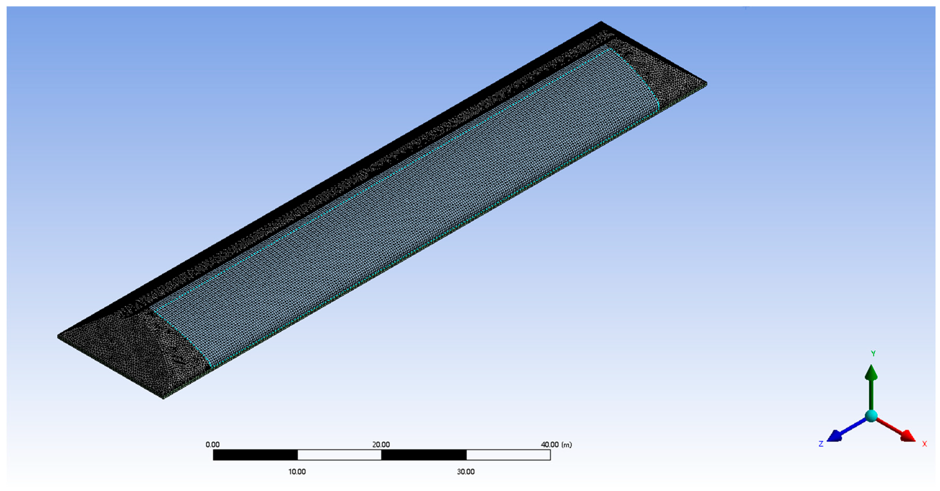
A three-dimensional model of the solar greenhouse was established using SOLIDWORKS 2016, with Fluent 19.0 employed to conduct numerical calculations. The grid size of the three-dimensional model was set to 0.3 m, with the maximum internal size set to 0.3 m. Following the division of the grid, the three-dimensional model is presented in Figure 5.
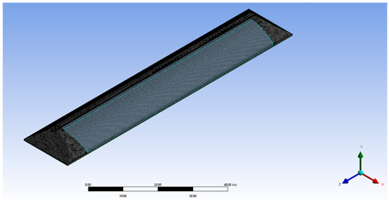

Figure 5.
Grid results and quality.
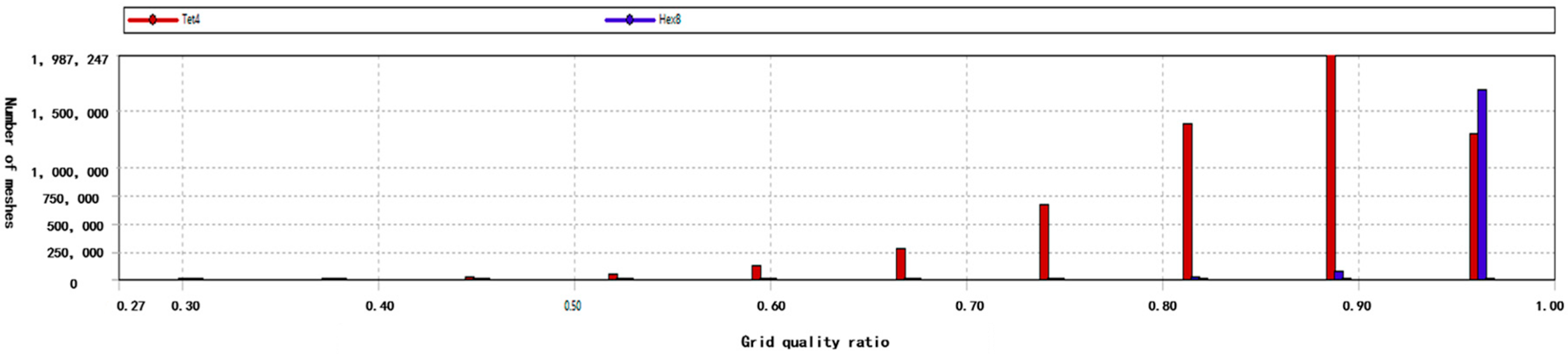
The quality of the gridding was evaluated based on the cell mass, with the majority of grids exhibiting a cell mass of 0.84 or above, and over 90% of the grids having a cell mass of less than 0.3 m. The model was constructed entirely of 717,866 grid cells, with no instances of negative grid errors, and it met the specifications of the FLUENT simulation tests.
2.3.2. Boundary Condition
This study analyzed the state of the indoor air temperature field in stratified partitions, set up as a transient model considering the energy equation and a DO solar radiation model. The temperature values of each boundary, such as backslope, floor, and fluid domains, are defined separately with the experimental data; the initial temperature values of each air boundary are shown in Table 3.
Table 3.
Thermophysical properties of materials.
For the other boundary walls, the initialized temperature value was 21.6 °C, and the temperature was initialized locally for the regions that need to be solved accurately in order to maximize the fit to the actual conditions of the initial temperature change. Appropriate material parameters were selected and the thermophysical properties of each material were listed in Table 4. According to the thermophysical properties of the materials and the boundary conditions, numerical calculations were performed from 16:00 on 1 January 2024 to 9:00 on 2 January 2024 for the entire computational domain to obtain the temperature changes in each region for 17 h.
Table 4.
Marginal areas of low temperature under the film on the lowest-temperature days in different months.
2.4. Python-Based Classification and Prediction Model for Measuring Points
2.4.1. K-Means Classification
K-means clustering is a typical algorithm in unsupervised learning that is used to divide data points into a pre-specified number of clusters [38]. Points within each cluster are relatively more similar to each other than points in other clusters. The algorithm initiates the process by randomly selecting K points as initial centers of mass. Subsequently, the data points are classified into the nearest clusters according to their Euclidean distance to these centers. Subsequently, the algorithm recalculates the center of mass of each cluster and reclassifies the data points based on the new center of mass. This process is repeated iteratively until the magnitude of the change in the center of mass is reduced to below a predetermined threshold, or until a preset number of iterations has been reached, ensuring that the Intra-cluster homogeneity is maximized.
The elbow method, which determines the optimal number of clusters by monitoring the rate of reduction in differences within the clusters, is employed in order to ascertain the number of classifications that was most appropriate for k-means clustering. The total sum of squared errors (SSE) was calculated for different numbers of clusters, with the aim of identifying an ‘elbow point’. This is defined as the point where the decrease in SSE becomes significantly smaller when the number of clusters increases.
The k-means method was utilized to analyze the clustering of temperatures at distinct measurement points within the shed film as well as at varying heights along a single measurement line. This analysis aimed to identify the smallest measurement line that is comparable to the 16th line, which represented the maximum spatial range of the region exhibiting the lowest temperatures. On the basis of these findings, all the points at this span and at line 16 were classified, and the lowest point height, y1, was identified to be of a similar category to that of the point at the shed film at line 16. The same methodology determines that the lowest measuring point height (y2) of the same category is the measuring point at the shed film of the measuring line at the above span. The low-temperature zone comprised the following elements: the arch frame line; the measurement point y1 at height No. 16, which was comparable to the temperature of the measurement point at the trellis film; the span of the measurement point No. 16, which was analogous to the aforementioned temperature; and the point y2 at height No. x2, which was analogous to the aforementioned temperature. As shown in Figure 6.

Figure 6.
Schematic representation of greenhouse high- and low-temperature thresholds in cluster analysis.
2.4.2. LSTM Prediction Model
A Long Short-Term Memory (LSTM) neural network is a special type of recurrent neural network that has a greater advantage in dealing with events with very long delays and prediction intervals, enabling multivariate time series prediction and providing technical support for precise temperature regulation and early warning in solar greenhouse [39].
The current study employed an LSTM model to predict and analyze temperatures at specific measurement points within the low-temperature region beneath a solar greenhouse film. The model employed a two-variable approach, incorporating the internal temperature of the greenhouse and time, to forecast future internal temperatures. This was achieved by utilizing historical temperature data from inside the greenhouse, thereby providing an early warning for temperature anomalies within the solar greenhouse.
The principal hyperparameters of the LSTM model included the model structure, optimizer parameters, and the number of training rounds. The model structure comprised two LSTM layers, each containing 50 units. The optimizer used was Adam with a learning rate of 0.001. The number of training rounds (epochs) was set to 20, with a batch size of 32. The dataset was divided into three distinct sets: training, test, and validation. The ratio of the training set to the test set was 8:1, and the ratio of the test set to the validation set was 1:1.
To control newly added cell states, LSTM uses three control switches: input gate, output gate, and forget gate. The input gate is used to control the input of information, the output gate is used to control the output of information, and the forgetting gate determines the retention of cell state history information.
Assuming that the model input is (x1, x2, …, xt) and the hidden layer output is (h1, h2, …, ht), there are three inputs to the LSTM at time t: the current network input xt, the hidden layer cell output ht-1 from the previous time, and the cell state ct-1 from the previous time. The expression of this equation is shown in (1):
where f denotes the forgetting gate; i denotes the input gate; c denotes the current cell state; o denotes the output gate; ht denotes the output of the LSTM cell at time t; W is the matrix of weight coefficients; b is the bias term; t denotes the time series; is the sigmoid activation function; tanh is the hyperbolic tangent activation function.
Prior to analysis, the experimental data underwent pre-processing, which involved the identification and removal of outliers and the standardization of temperature data at the measurement points. In the event of missing values or outliers, the average of the two preceding and subsequent values was employed as a replacement for the value in question. The formula that is used to normalize the data was shown in (2):
where Xpar represents the data after normalization; X represents the original data; Xmax is the maximum value in the original dataset; Xmin is the minimum value in the original dataset.
Mean absolute error (MAE), mean square error (MSE), and coefficient of determination (R2) were used as indicators for model evaluation. The expression of this equation is shown in (3):
where yi represents the experimental data, is the predicted value, and is the mean value.
3. Results
The dataset for analysis was selected from the period between 2 January 2024 at 09:00 and 18:00. This period coincided with the opening of the quilt and the exposure of the greenhouse to sunlight, although the top and bottom vents were not opened.
3.1. Indoor and Outdoor Light Temperature and Gas Change Rule
3.1.1. Indoor Light Temperature Change Rule
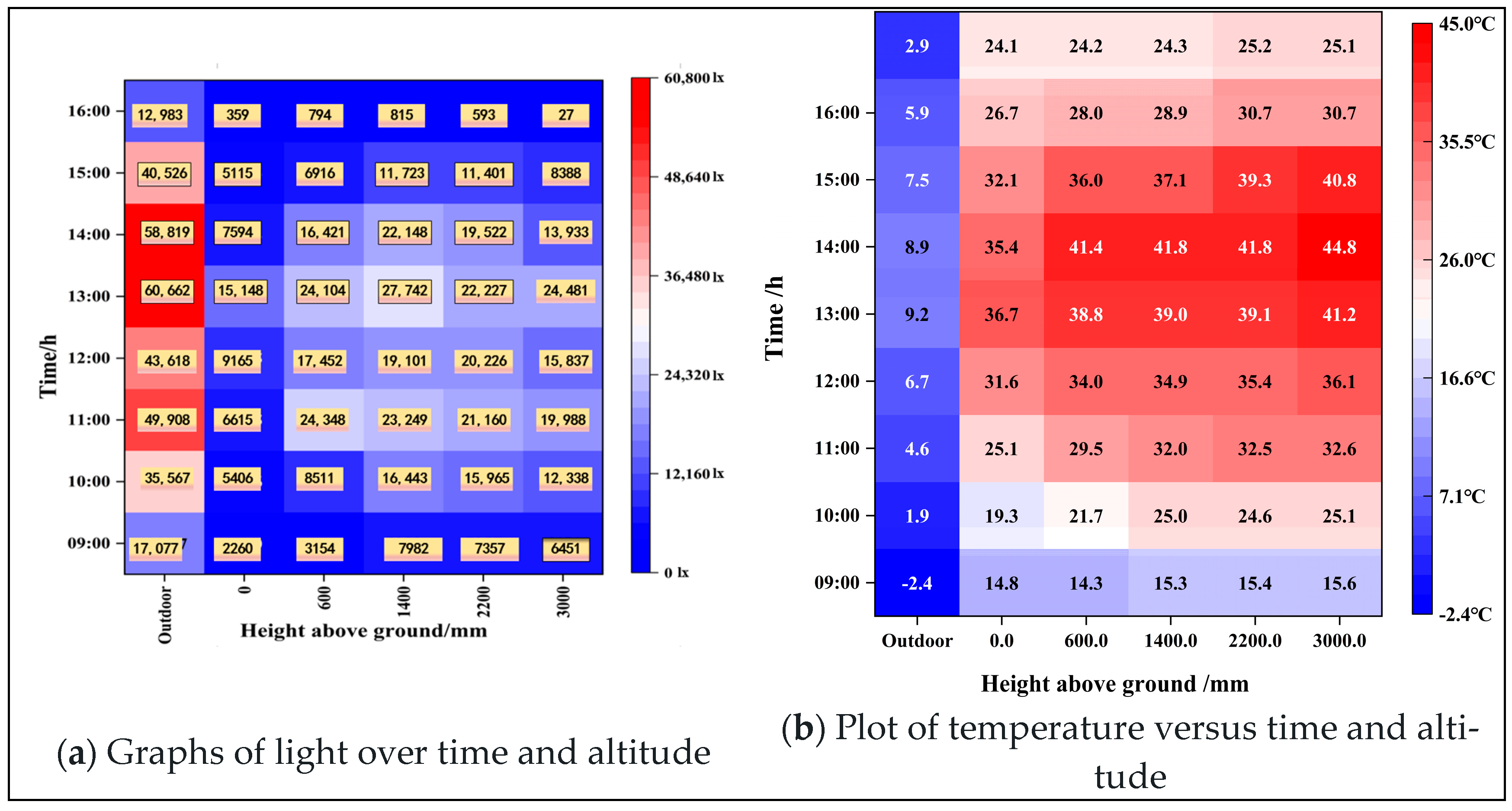
The data from the five measuring points that received light for the period under the condition after opening the shed film were analyzed, and, from Figure 7, it can be seen that, at the same time, as the height of the measurement point from the ground increased, the light first increased and then decreased due to the fact that the light at the measurement point at y = 3000 was affected by the fact that it is located at the lower end of the arch, and the arch shades the light more. At 12:00, the light intensity at y = 2200 was higher than at lower points in the same time period, while at other times it was lower than at lower points in the same time period. The analysis of the data for other months based on this phenomenon shows consistent results due to the fact that the arch blocks direct sunlight from this location most of the time and receives direct sunlight at 12:00 noon.
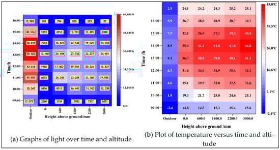
Figure 7.
Illumination temperature varying with time and altitude.
Over the same period of time, the temperature gradually increased as the measuring point rose due to the fact that the higher measuring points received more solar radiation and the lower measuring points were more shaded by vegetation. The temperature increased and then decreased with time at the same height point, which also indicated that the height point receives more solar radiation. Temperature change was due to the measurement point to receive solar radiation and external heat transfer of the two interacting structures; the solar radiation first increased and then decreased and the external heat transfer is in the increasing weight, so the temperature first increased and then decreased, the closer to the film the faster the temperature drop.
The data were analyzed by dividing the 9:00–16:00 time period into three segments based on the sunlight intensity and temperature variations. During the 9:00–13:00 period, the cumulative increase in outdoor light was 206,831 lx, with a corresponding increase in sunlight intensity at y-values of 0 mm, 600 mm, 1400 mm, and 2200 mm. The sunlight intensity at a y-value of 3300 mm increased by 38593 lx, 7569 lx, 94517 lx, 86935 lx, and 76096 lx, respectively. As the y-value increased, the sunlight intensity exhibited a biphasic response, initially increasing and subsequently decreasing. From 9:00 to 13:00, the outdoor temperature increased by 11.6 °C, and the temperature increased by 21.9 °C, 24.5 °C, 23.8 °C, 23.7 °C, and 25 °C. The temperature reached 69 °C at x = 6130 mm, y-value 0 mm, 600 mm, 1400 mm, 2200 mm, and 3300 mm, respectively. With the increase in the y-value, the temperature gradually increased. The highest temperature at 3300 mm was 41.24 °C. The data indicate that the highest point receives the greatest sunlight intensity, while the lower levels of light at y = 200 mm and y = 3000 mm are likely due to the shading from the arch. In addition, the heat in a greenhouse is distributed in space. Hotter air is less dense than colder air and tends to move to higher levels closer to the ceiling, while colder air remains at lower levels of the volume within the greenhouse.
During the period between 13:00 and 14:00, the cumulative increase in the outdoor sunlight intensity was 119,480 lx, while the indoor sunlight intensity was approximately 22,000 lx. The x-value was 6130 mm, while the y-values were 22,742 lx, 50,524 lx, 49,889 lx, 41,748 lx, and 35,414 lx. During the period between 13:00 and 14:00, the outdoor temperature increased by 1.3 °C, and the temperature increased by 1.3 °C, 2.6 °C, 2.8 °C, 2.7 °C, and 3.6 °C at x = 6130 mm and y-values of 0 mm, 600 mm, 1400 mm, 2200 mm, and 3300 mm, respectively. Furthermore, the temperature at the point in question was measured at several other locations. These included an outdoor temperature of 9 °C at a distance of 6130 mm from the surface in a horizontal plane, at a height of 0 mm, and a temperature of 36.7 °C. The point of measurement was subjected to an absorption of sunlight intensity of 22,742 lx, which was indicative of the downward trend in temperature.
The cumulative increase in the outdoor sunlight intensity during the 14:00–16:00 time period was 11,2327 lx. The x-values were 6130 mm, 13067 lx, 24,130 lx, 34,685 lx, and 31,516 lx at 0 mm, 600 mm, 1400 mm, 2200 mm, and 3300 mm, respectively. During the period from 14:00 to 16:00, the outdoor temperature decreased by 3.1 °C. The temperatures at x = 6130 mm, y-values of 0 mm, 600 mm, 1400 mm, 2200 mm, and 3300 mm decreased by 8.6 °C, 13.3 °C, 12.9 °C, 11.1 °C, and 14.1 °C, respectively. This indicates that sunlight intensity below 10,000 lx in the greenhouse during this period was insufficient to increase the indoor temperature. Therefore, supplemental light was required to reduce the temperature loss and increase the efficiency of photosynthesis.
3.1.2. The Pattern of Change in the Concentration of Carbon Dioxide (CO2) Indoor
The process of photosynthesis is one of energy conversion, with the total reaction of photosynthesis being heat absorption. Furthermore, the photosynthetic activity of crops affects the temperature distribution within a greenhouse. CO2 is a reactant in photosynthesis and its concentration affects the rate of photosynthesis in plants. Consequently, the concentration of CO2 affects the extent of the daytime high-temperature zone in solar greenhouses.
During the night, plants engage in respiration, resulting in the production of a considerable quantity of CO2 in the solar greenhouse, which has a higher molecular mass than the average molecular mass of air. The higher temperatures that occur near the surface of the solar greenhouse at night, coupled with the upward flow of hot air, which is impeded by CO2 due to its higher molecular mass, serve to exacerbate the low-temperature area that is under the solar greenhouse canopy at night.
On 1 January 2024, the greenhouses were covered with quilts between the hours of 17:00 and 09:00. As illustrated in Figure 8, during this period, indoor crop respiration was observed, with the outdoor CO2 levels recorded at approximately 450 ppm, a reduction of 28 ppm. The CO2 content increased by 277 ppm, 300 ppm, 319 ppm, 358 ppm, and 295 ppm at x = 6130 mm, y-values of 0 mm, 600 mm, 1400 mm, 2200 mm, and 3300 mm, respectively. The maximum value of 654 ppm was observed near the surface.
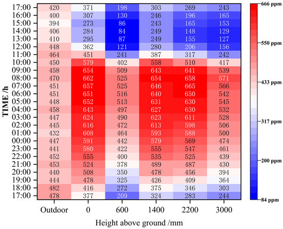
Figure 8.
Illustrates the CO2 levels over the course of 1 January 2024 from 17:00 to 4 January 2024 at 17:00.
The concentration of carbon dioxide in the atmosphere outdoors was approximately 420 parts per million (ppm) between 9:00 and 13:00, a reduction of 48 ppm. Inside the greenhouse, the CO2 levels increased by 359 ppm, 422 ppm, 394 ppm, 486 ppm, and 412 ppm at x = 6130 mm and y values of 0 mm, 600 mm, 1400 mm, 2200 mm, and 3300 mm. The lowest value of 87 ppm CO2 was recorded at a height of 600 mm above the ground surface, within the optimal growing range of the crop. It was recommended that CO2 be supplemented initially during this phase, with the temperature reaching up to 40 °C in the later crop growth range. This occurred when the crop was dormant due to the elevated temperatures.
A series of measurements were conducted between 13:00 and 14:00. The CO2 content at each measurement point was recorded as 284 ppm, 84 ppm, 249 ppm, 148 ppm, and 129 ppm at x = 6130 mm, and y-values of 0 mm, 600 mm, 1400 mm, 2200 mm, and 3300 mm, respectively. The lowest carbon dioxide point was 84 ppm at y = 600 mm within the crop height range. The location in question is situated within the optimal height range for crop growth, which enables the plants to absorb more CO2 through photosynthesis. Concomitantly, the hot air tends to ascend, and the upward movement of the air carries away a portion of the CO2 content, thereby reducing its concentration. The highest value was 284 ppm at y = 0 mm, which was above the threshold for the crop to remain dormant during this period. According to relevant studies [40], the appropriate concentration of carbon dioxide for cucumber photosynthesis is 1200–2000 ppm.
The CO2 level was recorded at 14:00–16:00, with an outdoor CO2 level of approximately 390 ppm, a decrease of 6 ppm. The concentration of CO2 increased by 23 ppm, 46 ppm, 3 ppm, 48 ppm, and 36 ppm at a distance of 6130 mm and a height of 0 mm, 600 mm, 1400 mm, 2200 mm, and 3300 mm, respectively. The lowest value was 130 ppm at y = 600 mm, which is within the optimal range for the crop’s growth. The highest value was 307 ppm at y = 0 mm. The CO2 content of the crop from respiration and the CO2 content from photosynthesis were approximately equal during this phase. At this stage, supplemental light can be applied in order to enhance the photosynthetic efficiency of the crop.
3.2. Law of Change of Indoor and Outdoor Temperature
According to Cheng [41] et al., the indoor temperature exhibited the greatest rate of change in the vertical direction, followed by the horizontal direction. However, the rate of change in the vertical direction can be considered negligible. A total of 93 measurement points within the indoor transverse interface across the center were analyzed in order to ascertain the temperature change patterns.
3.2.1. Overall Rate of Change of Indoor Temperature
Figure 9 illustrates the temperature fluctuations from 15:42 on 1 January 2024 to 16:00 on 2 January 2024 across a series of altitude measurement points within the greenhouse over the aforementioned period. As illustrated in Figure 9, the temperature exhibited a sharp decline following the placement of the quilts at 15:42, followed by a more gradual decline. This was attributed to the fact that the quilts impeded solar radiation, resulting in a general decrease in the temperatures within the greenhouse. The highest initial temperature at all the measurement points during the specified time period was 27.1 °C, while the lowest temperature was 19.3 °C. The maximum temperature difference between the measurement points was 7.8 °C. In the period under consideration, the lowest temperature recorded at the majority of the measurement points was at 6:48 on January 2, 2024, when the maximum temperature was 15 °C, the minimum temperature was 10.9 °C, and the maximum temperature difference between the measurement points was 4.1 °C. During this segment of the event, the maximum temperature drop at the measurement point was recorded at 13.2 °C, with the minimum drop being 6.9 °C. In this period, the temperatures recorded at the measurement points were averaged, resulting in a mean value of (14.33, 18.49) °C. This average was found to be approximately equal to the mean value of the other measurement points.

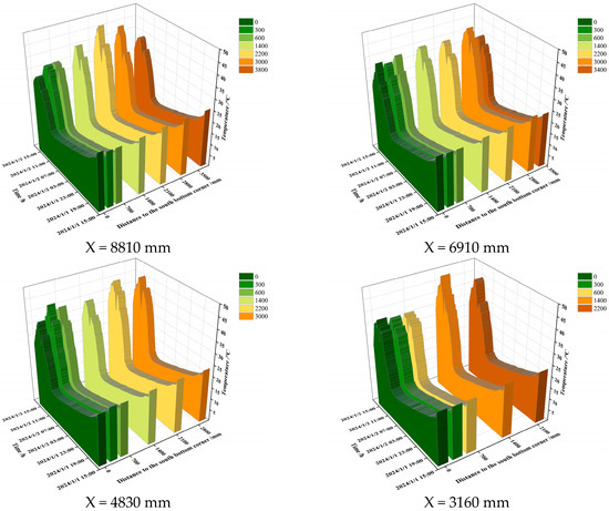
Figure 9.
Temperature change curves of indoor measuring points.
During the period between 07:00 and 12:00, there was a noticeable increase in light outside the building at approximately 07:00. However, the interior of the building remained unheated, with the quilts still rolled up, until the indoor temperature began to rise gradually, with a maximum temperature difference of 1.1 °C. At 09:00, the quilts were rolled up, resulting in a sharp increase in the indoor air temperature and the cessation of air vent operation. The maximum temperature of 43.3 °C was recorded at 11:54 at coordinates x = 2060 and y = 1400. The highest temperature recorded at the majority of the measuring points during the specified time period was observed at 11:54 on 2 January 2024, with a maximum temperature of 43.3 °C and a minimum temperature of 26.5 °C. The greatest temperature differential between the measuring points was 16.8 °C, which represents a considerable discrepancy in temperature. The temperature of the measurement points exhibited the greatest variation in the specified time period, with a maximum increase of 29.9 °C and a minimum decrease of 12.9 °C. The mean temperature of the measurement points was determined to be (17.16, 28.70) °C, with several points exhibiting nearly identical mean values.
The air temperature displayed a second increase between the hours of 12:00 and 14:30, reaching its highest value for the duration of the measurement period, with a peak temperature of 50.4 °C and a minimum of 26.4 °C. The temperature difference between the measurement points reached 24 °C, with the highest temperature recorded at 14:30. The maximum increase in temperature at the measurement point during the specified time period was 29.9 °C, while the minimum decrease was 12.9 °C. The temperature of the measurement points in this time period was averaged and the mean value was located at (29.85, 43.22) °C. There are measurement points with approximately equal mean values. The mean temperature of the measurement points over the specified time period was calculated by averaging the values. The resulting mean was found to be (29.85, 43.22) °C. There was a notable homogeneity in the mean values recorded across the measurement points.
The temperature curve exhibited a decline between 14:00 and 16:00, reaching a minimum at 16:00, with a maximum of 37.9 °C, a minimum of 22 °C, and a maximum temperature difference of 15.9 °C between the measurement points. The maximum temperature drop at the measurement point during the specified time period was 12.1 °C, while the minimum temperature drop was 4.4 °C. The temperature of the measurement points in this period was averaged, and the resulting mean value was located at (23.99, 43.70) °C. The mean values of the measurement points are approximately equal.
The preceding analysis revealed that the lowest temperature occurred at approximately 6:54 a.m., while the highest temperature was observed at 2:30 p.m. These times correspond to the periods of greatest light intensity within the greenhouse. In the event that the maximum temperature within the greenhouse exceeds 40 °C, it was advisable to ventilate the greenhouse. At different points in time, there were comparable temperature points. These were located at the lowest temperature at the membrane when the quilt was covered and at the highest temperature near the membrane when the quilt was rolled up and exposed to sunlight.
3.2.2. Temperature Change under the Film at Different Moments
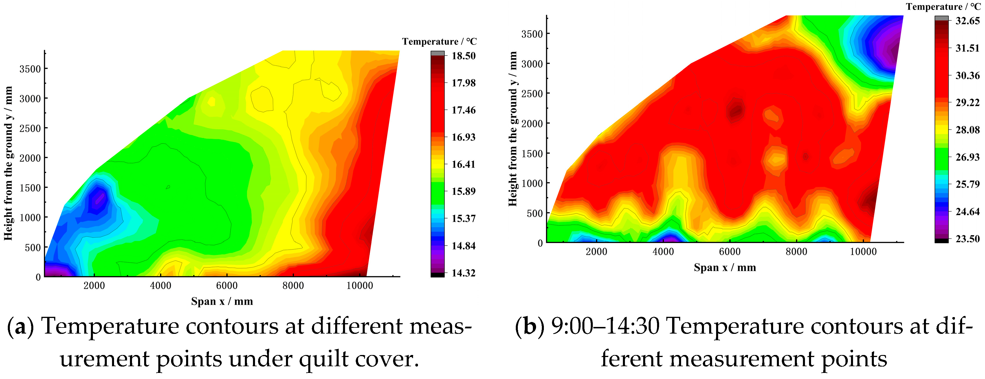
The mean temperature at each measurement point over the period from 16:00 on 1 January 2024 to 7:00 on 2 January 2024 (during which time the measurement point was covered with quilts, reaching a minimum temperature) and from 7:00 to 14:30 on 2 January 2024 (during which time the measurement point received solar radiation, reaching a maximum temperature) should be plotted on temperature contour graphs.
As can be seen in Figure 10, the area under the film exhibited a relatively uniform temperature distribution when the quilt was in the state of being covered. This area can be divided into four regions based on their thermal profiles: the southernmost region exhibited relatively low temperatures, while the northernmost region exhibited relatively high temperatures. In the state of receiving solar radiation, there were equal temperature measurement points in a certain area under the film. These measurement points can be divided into three parts, with the closer points to the film exhibiting the highest temperatures. During the solar radiation state, areas of lower temperature were observed on the northern wall due to the shielding effect of the quilts. This area was not directly exposed to solar radiation.
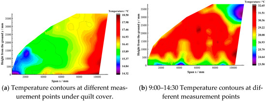
Figure 10.
Contour plots of the mean temperature at different time measurement points.
It was observed that, in the state of covering the quilt and receiving sunlight, there were low-temperature and high-temperature regions within the designated area under the film. The delineation of low-temperature and high-temperature areas under the two states can provide data support for the environmental regulation of solar greenhouses. Furthermore, the identification of low-temperature zones in solar greenhouses enables the provision of heating through a combination of blowers and ducting in climates with extreme temperatures, thereby ensuring the maintenance of suitable temperatures in areas dedicated to crop growth. Similarly, the identification of high-temperature zones in solar greenhouses permits the reduction in temperatures through the adjustment of the inlet wind speed, shading size, and air opening width, which results in the creation of an optimal temperature environment conducive to crop growth.
3.3. Marginal Effects under the Film
The results of previous research [38] indicated the presence of a region of low temperature beneath the solar greenhouse membrane. This region was centered on the span position at night and was situated at a distance of 2.7 m from ground level, at a height equivalent to the center of the membrane.
The measurement point situated at the same span of the film (the top) received a greater quantity of solar radiation and exchanged heat with the outdoor temperature more frequently. From Figure 11, it can be seen that the temperatures at the measurement points at the membrane were approximately equal. Consequently, the temperatures at the measurement points at different spans of the membrane were analyzed, and the locations of the low- and high-temperature spans at the membrane were defined. A comparative analysis of the temperatures at different heights of measurement points at the corresponding span positions on this basis was required in order to determine the heights of low and high temperatures at the corresponding spans. The highest-temperature region in a solar greenhouse is the high-temperature boundary region under the day film, and the lowest-temperature region in a solar greenhouse is the low-temperature boundary region under the night film. These boundary regions are composed of horizontal and vertical boundary points in the greenhouse.
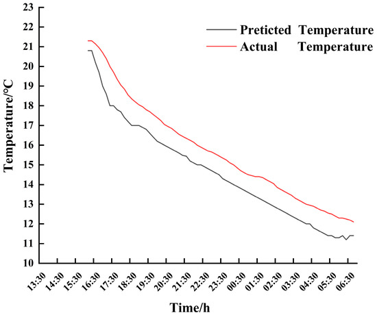
Figure 11.
Diagram of CFD temperature data and actual temperature data.
3.3.1. Marginal Effect Boundary Points under the Film
The temperature of the air within an indoor area was found to be influenced by the temperature of the outdoor air. The coordinates of the point at the highest point of the film in the line of measurement (17 lines) are as follows: () (: the number of the point at the top of the line of measurement). As the value of i decreases gradually, the values of approach the ridge height of the greenhouse. Measurement point 16–1 represented the lowest recorded night-time temperature in the entire dataset. To ascertain the equivalence of the temperatures recorded at the remaining measurement points, these values were compared to the temperature at point 16–1. This analysis led to the conclusion that the temperatures at these other measurement points were approximately equivalent to point 16–1. Consequently, the coordinates of the line with a temperature matching that recorded at point 16–1 were defined as the boundary of the low-temperature region in question. This will enable the position of the span of the low-temperature region under the film for x to be determined. On the basis of this analysis, the temperatures of the different measurement points at this span position and at the southernmost line were defined. These measurements were used to determine the height of the measurement points that corresponded to the temperature at the shed film. This information was used to define the height of the low-temperature measurement point at the southernmost 16 lines, y1, and to define the height of the low-temperature region at span x, y2. The boundary points and arches described previously were connected to form the low-temperature zone of the greenhouse, which was then covered with quilts.
3.3.2. Marginal Regions of Low Temperature under the Shed Film for Temperature Minima in Different Months
The data on the temperature minimums during the overwintering period, December 2023–March 2024, were analyzed to determine the optimal number of clusters at varying distances based on the elbow method in the k-means model. The three clusters were identified as being located close to the trellis (area of the lowest temperatures), close to the north wall (where the temperatures were the highest throughout the cross-section), and in the middle of the cross-section (area of the higher temperatures). The optimal number of clusters at the height distance was determined to be two classes.
According to the above study, during the overwintering period at night, with the same height near the north wall, the temperature was higher than that of the same span near the shed film at the point of measurement. Conversely, the temperature of the shed film at the lowest point was lower. This rule of change was applied to determine the low-temperature cut-off span of the cross-section in question. This was achieved by measuring the temperatures at different points along the film x2. The low-temperature boundary height, y2, at the x2 span was determined by comparing the temperatures at different heights of the x2 gauge line with the temperatures at the gauge points at the trellis membrane.
In accordance with the methodology for defining the lowest-temperature zones inside the greenhouse, the low-temperature zones for a period of 24 h beginning at midnight on the following day with the lowest average temperature value were established. The lowest-temperature zones were defined in the table below.
As can be seen from Table 5, the indoor low-temperature zone boundary was different in the case of the minimum temperature in different months during the overwintering period, with the minimum boundary distance from the south side foot level being 4830 mm and the longest boundary distance from the south side foot level being 6130 mm. The boundaries of the mesothermal region exhibited considerable variability. The minimum boundary was 6130 mm, the maximum boundary was 9820 mm, and the maximum boundary was situated in close proximity to the surface of the north wall. The minimum temperature recorded at the trellis film at the boundary of the low-temperature region was 4.2 °C, while the maximum temperature was 12 °C. The minimum temperature of the shed film at the boundary of the low-temperature region was 4.2 °C, with a maximum temperature of 12 °C. The lowest value was 7.6 °C and the highest was 12.1 °C at the trellis in the medium-temperature region.
Table 5.
Marginal areas of high temperature under the film on the hottest-temperature days in different months.
Once the boundary conditions of the cryogenic region have been established, the height at the cut-off position of the cryogenic region can be determined. As can be seen from Table 5, the maximum height at the low-temperature cut-off span for different months was 900 mm and the minimum was 600 mm. The maximum temperature at the cut-off span and cut-off height of the low-temperature region in different months was 12.1 °C, while the minimum temperature was 4.3 °C.
In conclusion, during the overwintering period, for instance, in March, the X-value of the low-temperature region was observed at (0, 6130) mm and the height was recorded within the range of (900, 3000) mm. In comparison with the other months, the temperatures in this region were consistently below 12.1 °C, and the ranges of high- and low-temperature values were relatively similar. Consequently, low indoor temperatures during cold days have a detrimental effect on crop growth. It is therefore important to consider the implementation of heating measures.
3.3.3. Marginal Areas of High Temperatures under the Trellis Film for Temperature Maxima in Different Months
Measuring lines 0, 1, 2, 3, and 4 were located in the lower part of the upwind opening of the greenhouse; the upper measuring points of these lines were affected by the upwind opening and the temperatures were higher than 30 °C during this period, so the upper measuring points of these lines were treated as high-temperature areas. The high-temperature region was defined by selecting 10:00–14:30 on the days with high mean temperature values, and the high-temperature boundary region under the shed film with the highest temperature value in different months was defined by using the k-means method of spanning the region with height according to the method of determining the low-temperature region.
As can be seen from Table 5, the high-temperature range indoors was different during the overwintering period in the case of the highest temperature in different months, with the minimum cut-off horizontal distance of the high-temperature range being 6130 mm and the maximum cut-off horizontal distance being 8810 mm. The minimum horizontal distance for high-temperature areas was 1630 mm, and the maximum horizontal distance was 3720 mm. The minimum value of the temperature at the shed film in the high-temperature region was 37.6 °C, and the maximum temperature was 49.3 °C.
The heights at the start and cut-off positions of the high-temperature region can then be determined provided that the location of the high-temperature region line is determined. The height range for the high-temperature start position was (300, 1400) mm, and the height range for the low-temperature cut-off position was identical. As illustrated in Table 5, the mean temperature at the (x1, y1) measurement point ranged from 49 °C at the highest to 36.7 °C at the lowest, while the mean temperature at the (x2, y2) measurement point spanned from 51 °C at the highest to 40.3 °C at the lowest. In conclusion, during the period of high temperatures that occurred during the overwintering period, the temperature reached a maximum of 30 °C or above. Consequently, in order to optimize the solar radiation absorption within the greenhouse environment and to facilitate heat storage at night, it is essential to implement effective ventilation and cooling measures at around 10 a.m. This may involve enlarging the ventilation openings in response to high-temperature conditions.
In order to provide early warning of high and low temperatures, it was necessary to set up measuring points at x = 6130 mm and y = 1400 mm. This should be conducted in accordance with the boundary conditions of the high- and low-temperature zones, as well as the altitude.
3.4. CFD Numerical Simulation
3.4.1. Verification of Model Accuracy
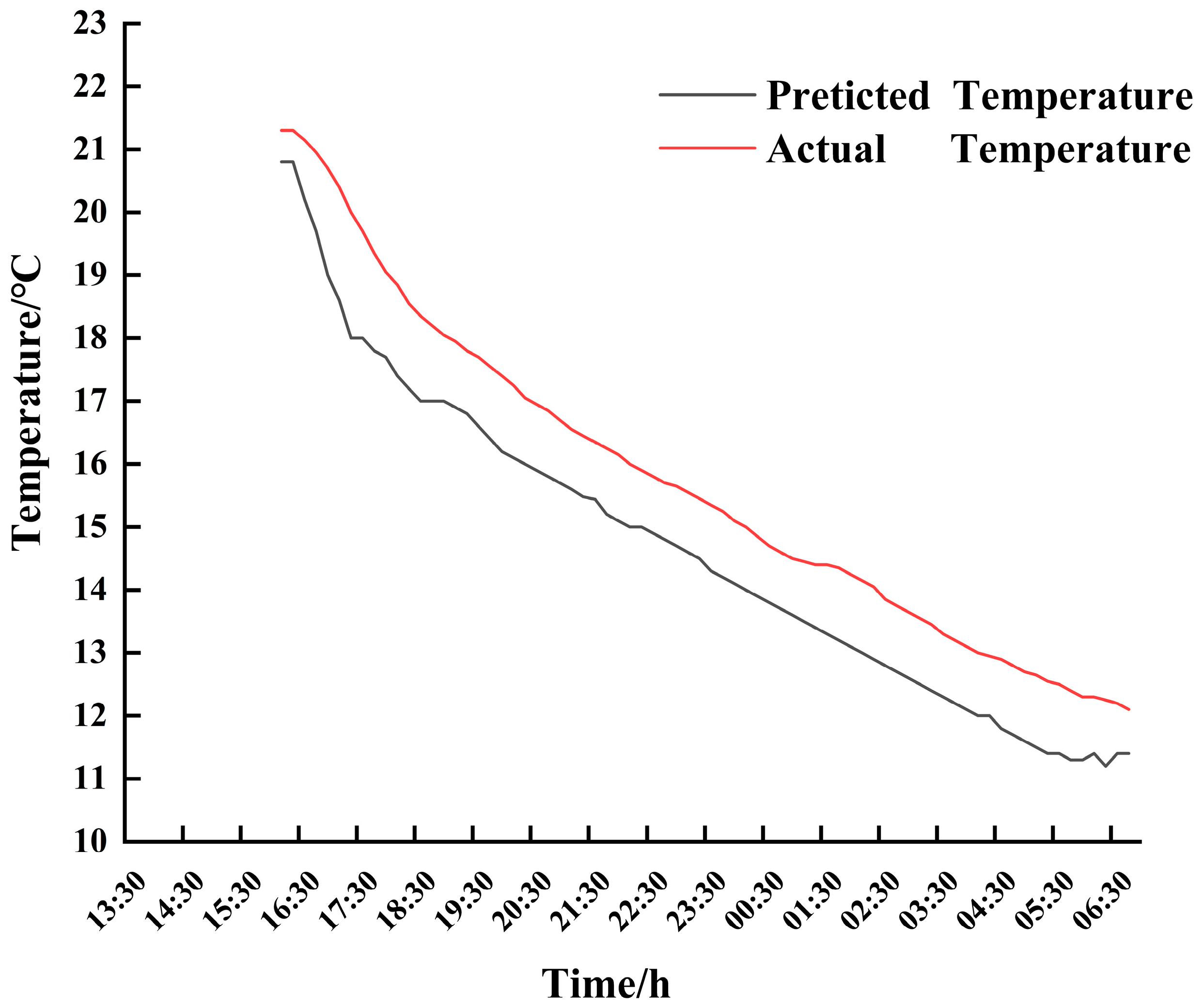
In order to verify the accuracy of the model, I selected the simulation data at the indoor measurement point (6130, 1400) in CFD 19.0-Post software to compare with the measured data at the same location. The time period is from 16:00 1 January 2024 to 7:00 2 January 2024.
The maximum discrepancy between the actual and predicted temperatures was 1.3°C, while the minimum discrepancy was 0.8 °C. The maximum absolute error was 8 percent, while the minimum absolute error was 6 percent. The model error range was within the controllable range, which indicated that the numerical simulation results were informative to a certain extent, and the distribution of the marginal area under the solar greenhouse film could be analyzed according to the numerical simulation calculation results.
3.4.2. Cloud View of Spatial Temperature Distribution at Different Moments across the Mid-Section
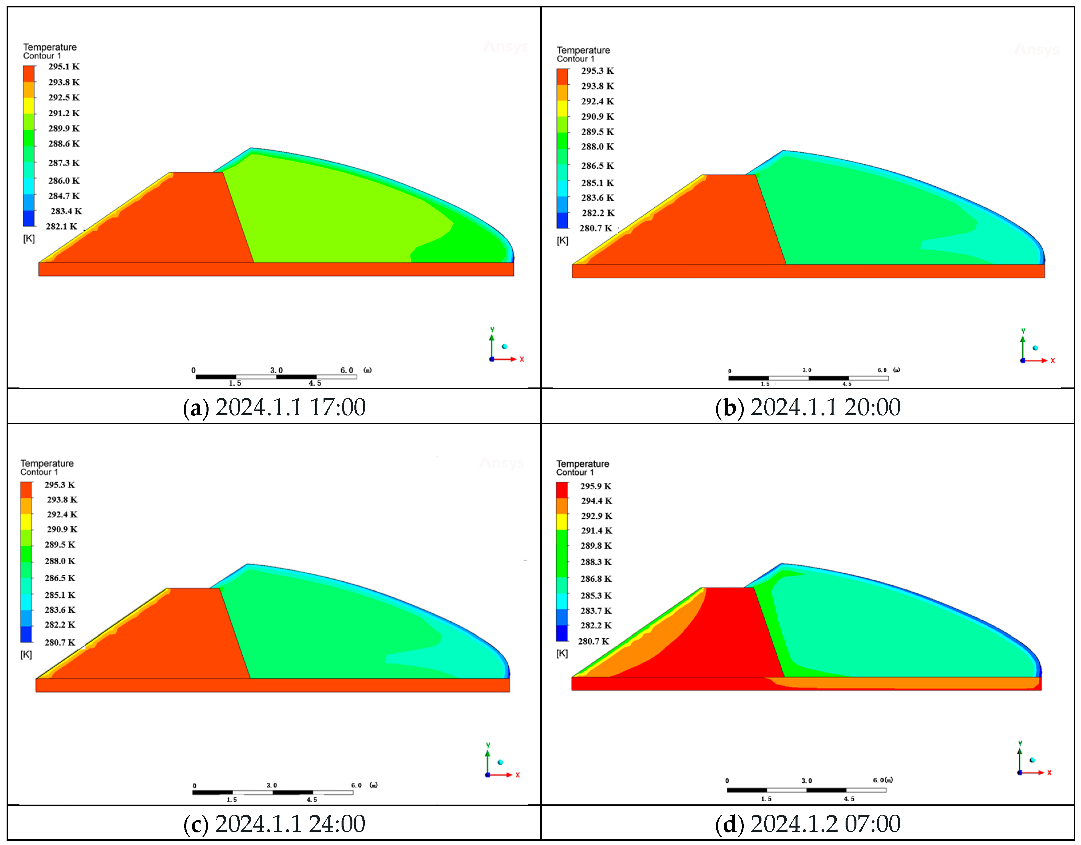
It can be seen from Figure 12 that the wall and soil temperatures were consistently higher than the air temperature throughout the duration of the numerical simulation. Furthermore, in a solar greenhouse, the greater the soil depth, the higher the soil temperature. A previous study [42] demonstrated that the soil temperature propagation distance exhibited a pronounced effect within a radius of 15 cm, with the temperature gradient gradually dissipating beyond a distance of 1 m. Consequently, this effect could be considered negligible in the latter region. From 16:00 on 1 January 2024, following the placement of the quilt, the area of the relatively low-temperature zone exhibited a gradual increase in extent over time. By 7:00 pm, the temperature within the entire greenhouse had reached a relatively low level. From a certain height above the shed membrane and from the south side of the bottom corner of a certain horizontal distance, the temperature was approximately equal to the region. This part of the region constitutes the shed membrane under the low-temperature marginal effect of the region, in accordance with the change rule of the experimental data.
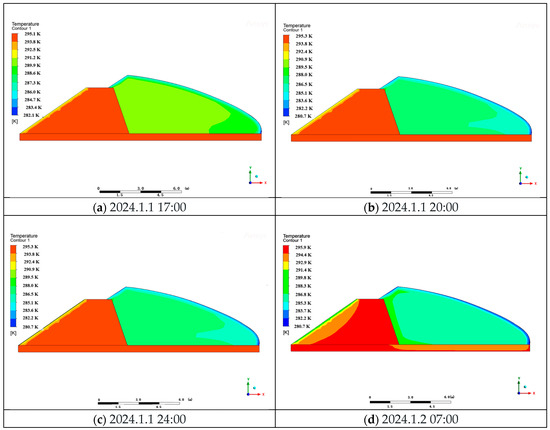
Figure 12.
Spatial distribution of temperature at different moments across the mid-section.
The air temperature in the lower areas under the film was lower than in other areas due to the lower thermal insulation performance of this area compared to other areas. The rate of thermal conductivity between the air at the membrane and the outdoor air also depended on the temperature difference between the indoor and outdoor conditions. This resulted in significant heat loss in this area. The air at the shed film absorbed the heat from the nearby higher-temperature air, and the rate of heat transfer from air to air depends on the magnitude of the temperature difference. As the height of the measurement point from the ground increased and the distance from the north wall was closer, it was evident that the rate of heat absorption at the measurement point had increased and that the rate of heat dissipation had decreased. It was also apparent that a portion of the air exhibited a greater rate of heat dissipation than heat absorption, which resulted in a portion of the cold area under the shedding membrane.
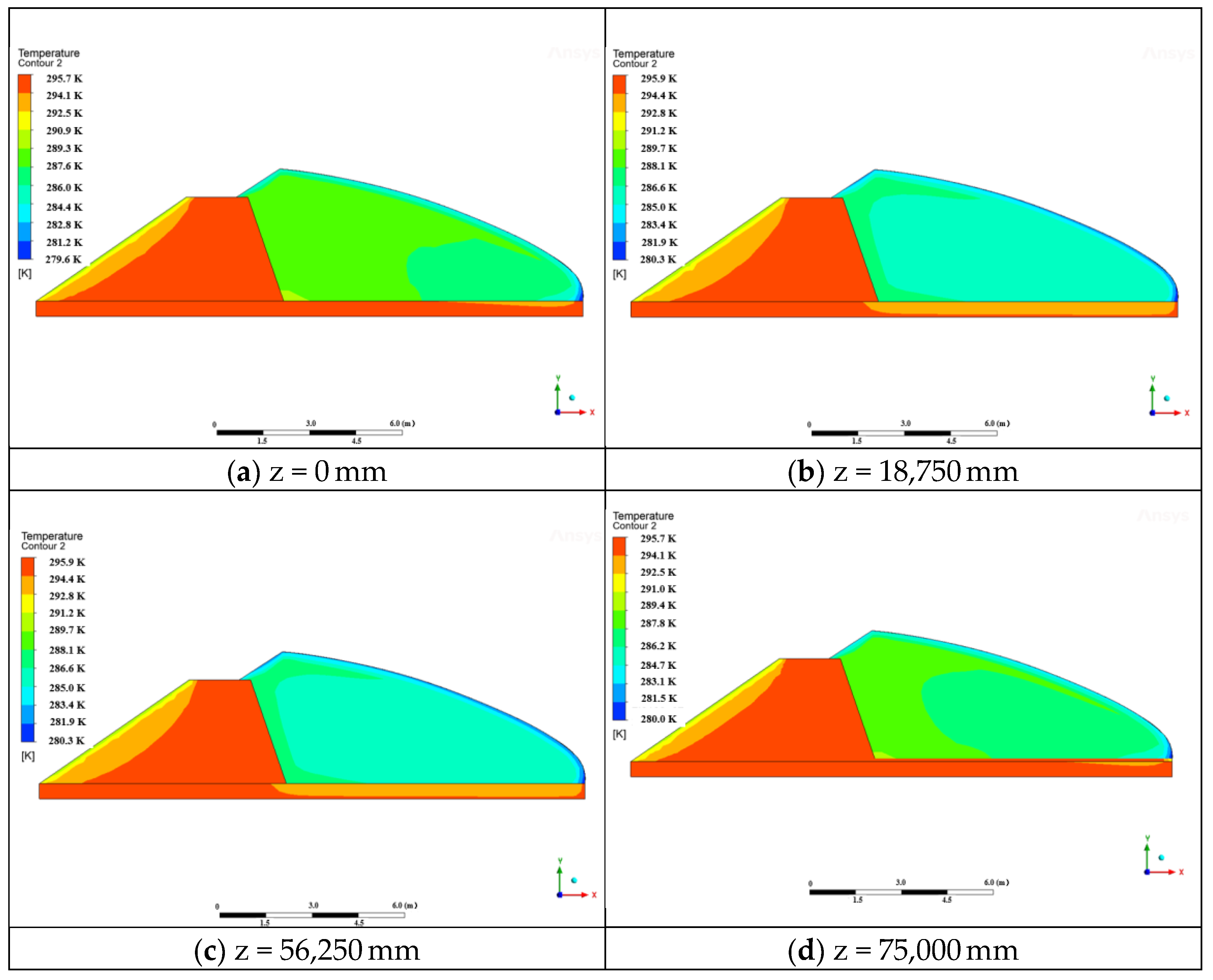
3.4.3. Distribution of Temperature across Different Spans at 07:00 am
As can be seen from Figure 13, at 7:00 a.m. on 2 January, the quilt was in the state of covering the sheath. The temperature of the low-temperature region under the sheath near the east and west walls was higher than that of the low-temperature region under the sheath in the middle cross-section. The closer the same span was to the middle section location, the greater the extent of the low-temperature region. Conversely, higher temperatures were observed near the north wall and near the soil.

Figure 13.
Distribution of temperatures in different spans at 07:00 a.m.
This was a consequence of the east and west walls functioning as exothermic bodies and the air temperature being higher in the vicinity of these walls. As the exothermic effect of the east and west walls diminished when the middle region was reached, it was important to pay particular attention to the temperature change in the span-center cross-section at night during the winter months. In light of the fact that an actual entrance was situated in close proximity to either the eastern or western wall, appropriate means of minimizing heat loss were installed in the vicinity of said entrance.
From the above temperature maps at different locations at the same time, and the temperature distribution maps at different times in the center section, it is clear that there was a specific area of low temperature from the bottom corner of the south side to near the north wall, within the area of the shelter foil.
3.5. LSTM Prediction Model
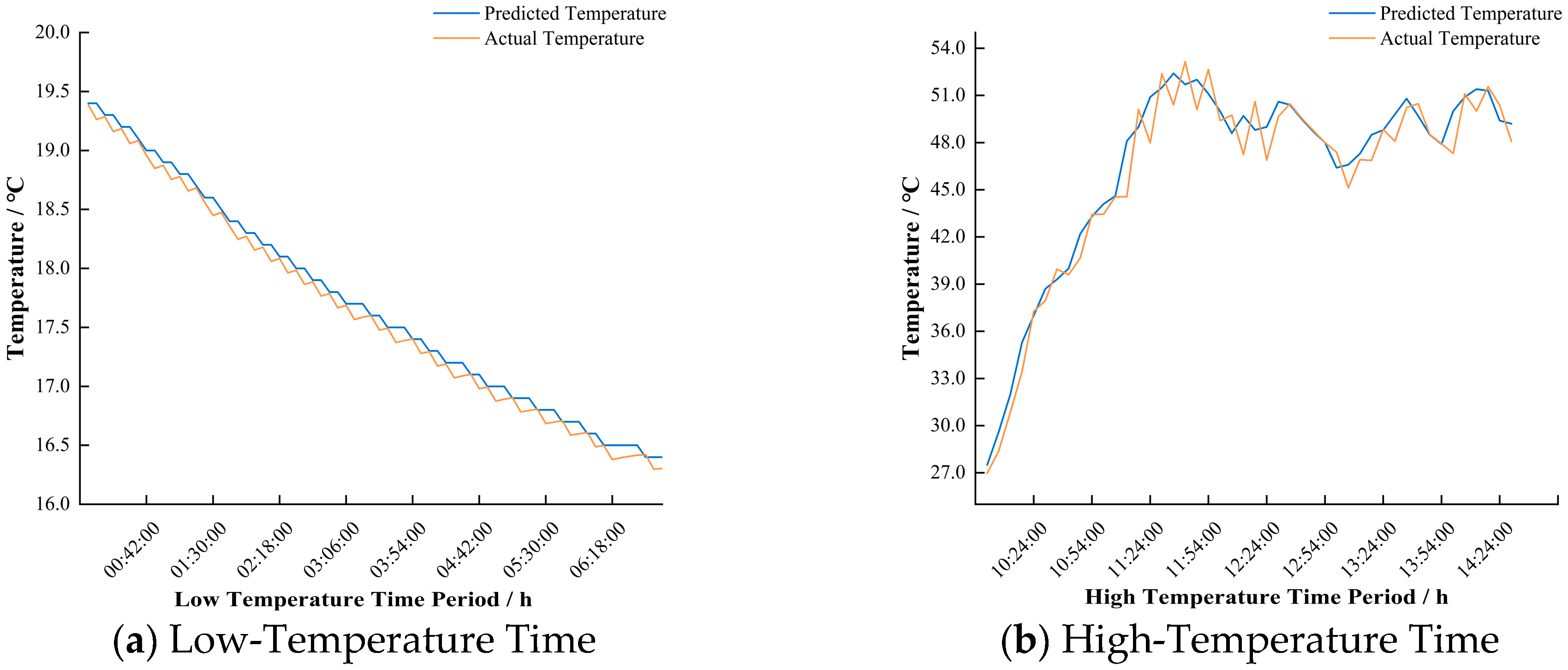
In order to predict the low-temperature and high-temperature zone points in a timely manner so that control measures can be adjusted to provide a suitable environment for crop growth, LSTM modelling of low- and high-temperature points was carried out in this study. For the prediction of the LSTM model, the measurement points of line 7 (span distance 6130 mm) were selected from 31 December 2023 to 28 February 2024. The temperature dataset of the key measurement point (6130, 1400) in the above study was selected for the training set loss, validation set loss, training set evaluation, and validation set evaluation for visualization and analysis, and the results are shown in Figure 14.
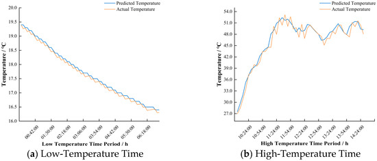
Figure 14.
Comparison of predicted and test temperature results for high- and low-temperature periods.
From the test results and the model prediction results, it can be seen that, in the low-temperature period, the air temperature was in a state of decline, the maximum temperature difference between the test temperature and the predicted temperature was 0.1529 °C, and the minimum error was 0.0221 °C; the model prediction results were better. During the high-temperature period, the air temperature first showed a significant increase and then fluctuated and changed after reaching the peak; the maximum temperature difference between the test temperature and the predicted temperature was 3.54 °C, the minimum temperature difference was 0 °C, and the difference between the test temperature and the predicted temperature was also relatively small.
In conclusion, the prediction results were more satisfactory in both the low- and high-temperature sections, so the LSTM model can be used to provide early warning for both low- and high-temperature control. By predicting the value and time of low and high temperatures in advance, the basis for precise greenhouse regulation is provided, thereby ensuring that the greenhouse provides a better growing environment for crops.
4. Conclusions
In this paper, the marginal effect under the solar greenhouse film has been studied and predicted, and its main results are as follows:
- (1)
- The maximum horizontal point of the cut-off position of the low-temperature region of the marginal effect under the wintering shed film was 6130 mm, while the minimum was 4830 mm. In the low-temperature zone of the marginal effect under the film, the maximum height at the cut-off horizontal position was 3000 mm, while the minimum height was 600 mm. The temperature in the low-temperature region under the greenhouse film during the overwintering period exhibited a marginal effect. The highest temperature was 12.1 °C, while the lowest temperature was 4.0 °C. Furthermore, the maximum temperature difference in the low-temperature region was 1 °C in the same time period in different months.
- (2)
- The minimum horizontal distance between the start of the high-temperature area of the marginal effect under the film and the bottom foot of the south side was 1630 mm, while the maximum horizontal distance was 8810 mm. The maximum height at the cut-off of the high-temperature region of the marginal effect under the film was 1400 mm, while the minimum height was 300 mm. The starting maximum height at the starting position of the high-temperature region under the film was 1400 mm, while the minimum height was 300 mm. The maximum temperature recorded during the overwintering season in the high-temperature region of the marginal effect under the film was 51 °C, with the minimum temperature being 36.7 °C. Furthermore, there was a maximum temperature difference of 7 °C between the same time period in different months.
- (3)
- The numerical simulations based on the CFD method yielded accurate results. However, low temperatures were observed in the areas in close proximity to the shed film.
- (4)
- The LSTM prediction model presented in this paper demonstrated a high degree of accuracy in forecasting the temperature within an experimental greenhouse. The model exhibited an average absolute error of 0.2410 °C, an average squared error of 0.2853 °C, and a coefficient of determination (R2) of 0.9869. The proposed prediction model is capable of forecasting the temperature of a solar greenhouse with an identical type of earthen wall in Shanxi, China. Furthermore, it can provide a buffer period for the temperature control of the greenhouse, which is essential for the efficient production of greenhouse crops.
This paper examined the marginal effect of the solar greenhouse membrane, focusing on the area where the marginal effect is formed under the membrane. However, it does not measure and analyze the night-time release of soil, the heat absorption by the wall, or the heat flow in the air. To gain a more comprehensive understanding of the marginal effect of the greenhouse film, future research should consider the arch structure, covering materials, soil heat absorption and release, and wall heat absorption and release. This would enable a more detailed analysis of the formation mechanism of the marginal effect of the greenhouse film as a whole.
Author Contributions
Conceptualization, W.C. and Y.W.; methodology, Y.W.; software, C.W.; validation, Y.W., C.W. and W.C.; formal analysis, Y.W.; investigation, Y.W.; resources, W.C.; data curation, Y.W.; writing—original draft preparation, W.C.; writing—review and editing, Z.L.; visualization, Y.W.; supervision, Z.L.; project administration, W.C.; funding acquisition, W.C. All authors have read and agreed to the published version of the manuscript.
Funding
This research was supported by the Upper-Level Project of the Shanxi Natural Science Foundation of China (No. 202103021223132; No. 202103021224151), the Graduate Scholarship Fund of Shanxi Agricultural University in China (2023BQ06), and the Youth Fund of National Natural Science in China (No. 42207102).
Institutional Review Board Statement
Not applicable.
Data Availability Statement
Data are contained within the article.
Conflicts of Interest
The authors declare no conflicts of interest.
References
- Lal, R. Home gardening and urban agriculture for advancing food and nutritional security in response to the COVID-19 pandemic. Food Secur. 2020, 12, 871–876. [Google Scholar] [CrossRef] [PubMed]
- Domenico, M.; Cristina, B.; Simone, P.; Congedo, P.M. Solar greenhouses: Climates, glass selection, and plant well-being. Sol. Energy 2021, 230, 222–241. [Google Scholar]
- Han, L. Reflections on the construction of facility agricultural engineering and agricultural modernisation. Agric. Technol. Equip. 2021, 10, 113–114. [Google Scholar]
- Dragićević, M.S. Determining the Optimum Orientation of a Greenhouse on the Basis of the Total Solar Radiation Availability. Therm. Sci. 2011, 15, 215–221. [Google Scholar] [CrossRef]
- Deng, L.; Huang, L.; Zhang, Y.; Li, A.; Gao, R.; Zhang, L.; Lei, W. Analytic model for calculation of soil temperature and heat balance of bare soil surface in solar greenhouse. Sol. Energy 2023, 249, 312–326. [Google Scholar] [CrossRef]
- Zhang, Y.; Henke, M.; Li, Y.; Xu, D.; Liu, A.; Liu, X.; Li, T. Towards the maximization of energy performance of an energy-saving Chinese solar greenhouse: A systematic analysis of common greenhouse shapes. Sol. Energy 2022, 236, 320–334. [Google Scholar] [CrossRef]
- Yan, D.; Hu, L.; Zhou, C. Structural performance analysis of elliptical tube single-tube arch daylight greenhouse. J. Agric. Eng. 2022, 38, 217–224. [Google Scholar]
- Lei, W.; Lu, H.; Qi, X.; Tai, C.; Fan, X.; Zhang, L. Field measurement of environmental parameters in solar greenhouses and analysis of the application of passive ventilation. Sol. Energy 2023, 263, 111851. [Google Scholar] [CrossRef]
- Wu, X.; Li, Y.; Jiang, L.; Wang, Y.; Liu, X.; Li, T. A systematic analysis of multiple structural parameters of Chinese solar greenhouse based on the thermal performance. Energy 2023, 273, 127193. [Google Scholar] [CrossRef]
- Zhang, Y.; Xu, L.; Zhu, X.; He, B.; Chen, Y. Thermal environment model construction of Chinese solar greenhouse based on temperature–wave interaction theory. Energy Build. 2023, 279, 112648. [Google Scholar] [CrossRef]
- Tawalbeh, M.; Aljaghoub, H.; Alami, A.H.; Olabi, A.G. Selection criteria of cooling technologies for sustainable greenhouses: A comprehensive review. Therm. Sci. Eng. Prog. 2023, 38, 101666. [Google Scholar] [CrossRef]
- Jiao, W.; Liu, Q.; Gao, L.; Liu, K.; Shi, R.; Ta, N. Computational Fluid Dynamics-Based Simulation of Crop Canopy Temperature and Humidity in Double-Film Solar Greenhouse. J. Sens. 2020, 2020, 8874468. [Google Scholar] [CrossRef]
- Wang, C.; Yang, S.; Chen, Z.; Xie, Z.; Zhang, Z. Effects of increased CO2 application and LED supplemental light interaction on photosynthesis and quality of chilli peppers. Fujian Agric. J. 2022, 37, 67–73. [Google Scholar]
- Singh, M.C.; Singh, K.G.; Singh, J.P. Performance of soilless cucumbers under partially controlled greenhouse environment in relation to deficit fertigation. Indian J. Hortic. 2018, 75, 259. [Google Scholar] [CrossRef]
- Zhao, L.; Lu, L.; Liu, H.; Li, Y.; Sun, Z.; Liu, X.; Li, T. A one-dimensional transient temperature prediction model for Chinese assembled solar greenhouses. Comput. Electron. Agric. 2023, 215, 108450. [Google Scholar] [CrossRef]
- Lee, C.K.; Chung, M.; Shin, K.-Y.; Im, Y.-H.; Yoon, S.-W. A study of the effects of enhanced uniformity control of greenhouse environment variables on crop growth. Energies 2019, 12, 1749. [Google Scholar] [CrossRef]
- Hu, J.; Fan, G.; Gao, Y. Experimental study on the characteristics of air temperature change in daylight greenhouse during overwintering period. J. Taiyuan Univ. Technol. 2014, 45, 6. [Google Scholar]
- Moore, C.E.; MeachamHensold, K.; Lemonnier, P.; Slattery, R.A.; Benjamin, C.; Bernacchi, C.J.; Lawson, T.; Cavanagh, A.P. The effect of increasing temperature on crop photosynthesis: From enzymes to ecosystems. J. Exp. Bot. 2021, 72, 2822–2844. [Google Scholar] [CrossRef] [PubMed]
- Chen, D.-S. Microclimate environment and its regulation in solar greenhouse. China Flower Hortic. 2005, 6, 47–52. [Google Scholar]
- Cheng, W.; Yu, W.; Wang, C.; Tao, W.; Junlin, H.E.; Liu, Z. Study study on the variation of thermal environment and photosynthesis characteristics of strawberry in a solar greenhouse. INMATEH—Agric. Eng. 2023, 70, 211–220. [Google Scholar] [CrossRef]
- Cheng, W.; Wang, C.; Wang, Y.; Cheng, M.; Qiao, P.; Liu, Z. Study of the Thermal Environment and Marginal Effects of a Sunken Solar Greenhouse. Eng. Agrícola Jaboticabal 2024, 44, e20230168. [Google Scholar] [CrossRef]
- Homa, E.; Ramin, R. Optimal design for solar greenhouses based on climate conditions. Renew. Energy 2020, 145, 1255–1265. [Google Scholar]
- Ahamed, M.S.; Guo, H.; Tanino, K. Sensitivity Analysis of CSGHEAT Model for Estimation of Heating Consumption in a Chinese-style Solar Greenhouse. Comput. Electron. Agric. 2018, 154, 99–111. [Google Scholar] [CrossRef]
- Hu, J.; Lei, W.; Lu, Y.; Wei, Z.; Liu, X.; Gao, M. Research on temperature prediction model of solar greenhouse based on 1D CNN-GRU. J. Agric. Mach. 2023, 54, 339–346. [Google Scholar]
- Zhang, C.; Wei, M.; Xu, P. Analysis of inverse temperature phenomenon in solar greenhouse based on soil heat storage. J. Shenyang Agric. Univ. 2019, 50, 114–119. [Google Scholar]
- Liu, Q.; Ta, N.; Jiao, W.; Kang, H.; Zhao, Z. Spatial and temporal distribution and prediction model of canopy temperature and humidity in solar greenhouse crops. North Hortic. 2019, 17, 56–65. [Google Scholar]
- Zhang, J.; Shen, K.; Chen, D.; Zhang, M.; Zhang, H.; Hu, J. Analysis of spatial and temporal variation rules of characteristic temperature of solar greenhouse canopy based on internet of things. J. Agric. Mach. 2021, 52, 335–342. [Google Scholar]
- Cheng, W.; Liu, Z. Study on the change rate of the indoor temperature of a sunken solar greenhouse. INMATEH-Agric. Eng. 2022, 68, 119–126. [Google Scholar] [CrossRef]
- Zhang, G.; Fu, Z.; Yang, M.; Liu, X.; Dong, Y.; Li, X. Nonlinear simulation for coupling modeling of air humidity and vent opening in Chinese solar greenhouse based on CFD. Comput. Electron. Agric. 2019, 162, 337–347. [Google Scholar] [CrossRef]
- Sun, S.; Dong, C.; Lai, Z.; Yang, H. Study on the internal temperature change of solar greenhouse under different ambient temperatures based on CFD. Tianjin Agric. Sci. 2020, 26, 5. [Google Scholar]
- Zhang, X.; Lv, J.; Xie, J.; Yu, J.; Zhang, J.; Tang, C.; Li, J.; He, Z.; Wang, C. Solar Radiation Allocation and Spatial Distribution in Chinese Solar Greenhouses: Model Development and Application. Energies 2020, 13, 1108. [Google Scholar] [CrossRef]
- Liu, Y.; Li, D.; Wan, S.; Wang, F.; Dou, W.; Xu, X.; Li, S.; Ma, R.; Qi, L. A long short-term memory-based model for greenhouse climate prediction. Int. J. Intell. Syst. 2021, 37, 135–151. [Google Scholar] [CrossRef]
- Dong, S.; Ahamed, M.S.; Ma, C.; Guo, H. A time-dependent model for predicting thermal environment of mono-slope solar greenhouses in cold regions. Energies 2021, 14, 5956. [Google Scholar] [CrossRef]
- Gong, J. Construction of Spatial Temperature Distribution Model in Solar Greenhouse. Ph.D. Thesis, Northwest Agriculture and Forestry University, Xianyang, China, 2023. [Google Scholar]
- Mahmood, F.; Govindan, R.; Bermak, A.; Yang, D.; Al-Ansari, T. Data driven robust model predictive control for greenhouse temperature control and energy utilisation assessment. Appl. Energy 2023, 343, 121190. [Google Scholar] [CrossRef]
- Jung, D.H.; Kim, H.S.; Jhin, C.; Kim, H.J.; Park, S.H. Time-serial analysis of deep neural network models for prediction of climatic conditions inside a greenhouse. Comput. Electron. Agric. 2020, 173, 105402. [Google Scholar] [CrossRef]
- Moon, T.; Lee, J.W.; Son, J.E. Accurate Imputation of Greenhouse Environment Data for Data Integrity Utilizing Two-Dimensional Convolutional Neural Networks. Sensors 2021, 21, 2187. [Google Scholar] [CrossRef] [PubMed]
- Laxmikant, D.; Jathar, K.N.; Awasarmol, U.V.; Gurav, R.; Patil, J.D.; Shahapurkar, K.; Soudagar, M.E.M.; Khan, T.M.Y.; Kalam, M.A.; Hnydiuk-Stefan, A.; et al. A comprehensive analysis of the emerging modern trends in research on photovoltaic systems and desalination in the era of artificial intelligence and machine learning. Heliyon 2024, 10, e25407. [Google Scholar]
- Yang, Y.; Gao, P.; Sun, Z.; Wang, H.; Lu, M.; Liu, Y.; Hu, J. Multistep ahead prediction of temperature and humidity in solar greenhouse based on FAM-LSTM model. Comput. Electron. Agric. 2023, 213, 108261. [Google Scholar] [CrossRef]
- Sun, W. Changing law of CO2 concentration and replenishment time of cucumber in sunlight greenhouse in Kazuo County. China Agric. Ext. 2020, 36, 67–68. [Google Scholar]
- Cheng, W.-W. Research on Three-Dimensional Thermal Environment and Marginal Effect of Sunken Solar Greenhouse. Ph.D. Thesis, Shanxi Agricultural University, Taiyuan, China, 2021. [Google Scholar]
- Yu, W.; Liu, W.; Bai, Y.; Ding, X. Simulating thermal environment in a two-span solar greenhouse using CFD. Trans. Chin. Soc. Agric. Eng. (Trans. CSAE) 2023, 39, 215–222. [Google Scholar]


Disclaimer/Publisher’s Note: The statements, opinions and data contained in all publications are solely those of the individual author(s) and contributor(s) and not of MDPI and/or the editor(s). MDPI and/or the editor(s) disclaim responsibility for any injury to people or property resulting from any ideas, methods, instructions or products referred to in the content. |
© 2024 by the authors. Licensee MDPI, Basel, Switzerland. This article is an open access article distributed under the terms and conditions of the Creative Commons Attribution (CC BY) license (https://creativecommons.org/licenses/by/4.0/).