
Early Crop Identification Study Based on Sentinel-1/2 Images with Feature Optimization Strategy


Abstract
1. Introduction
2. Study Area and Datasets
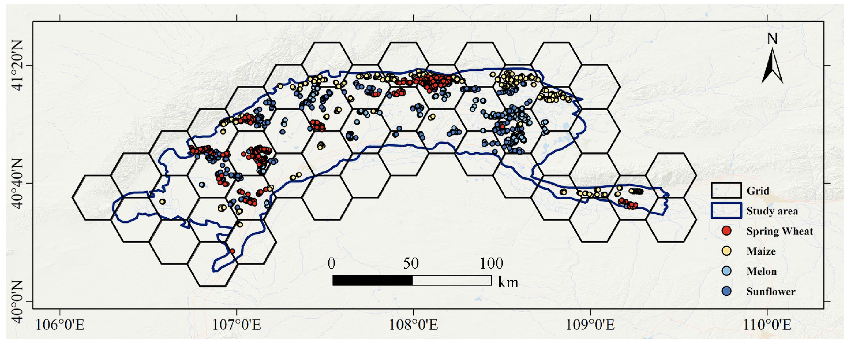
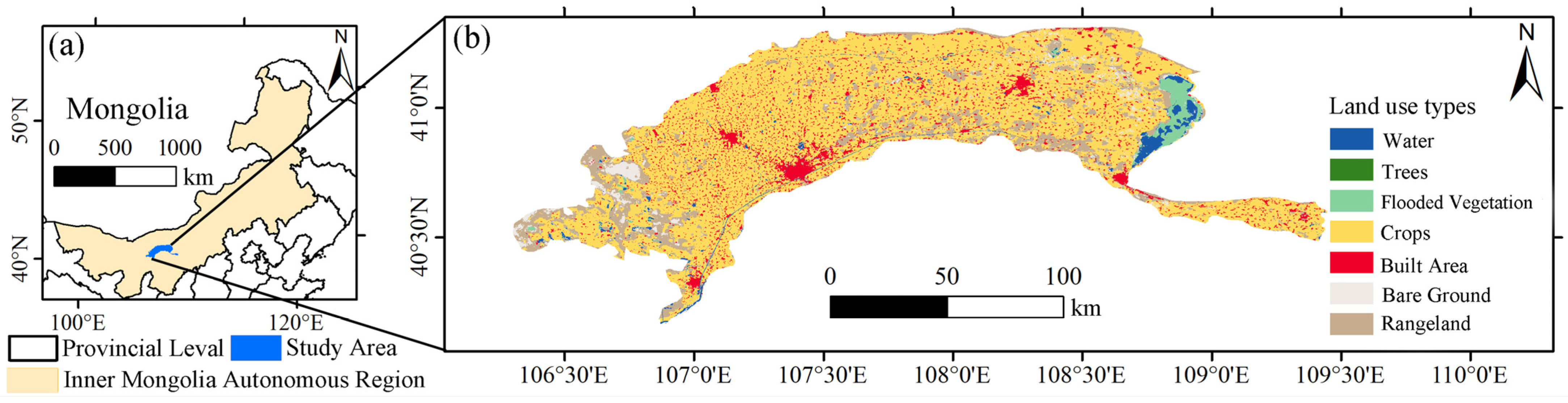
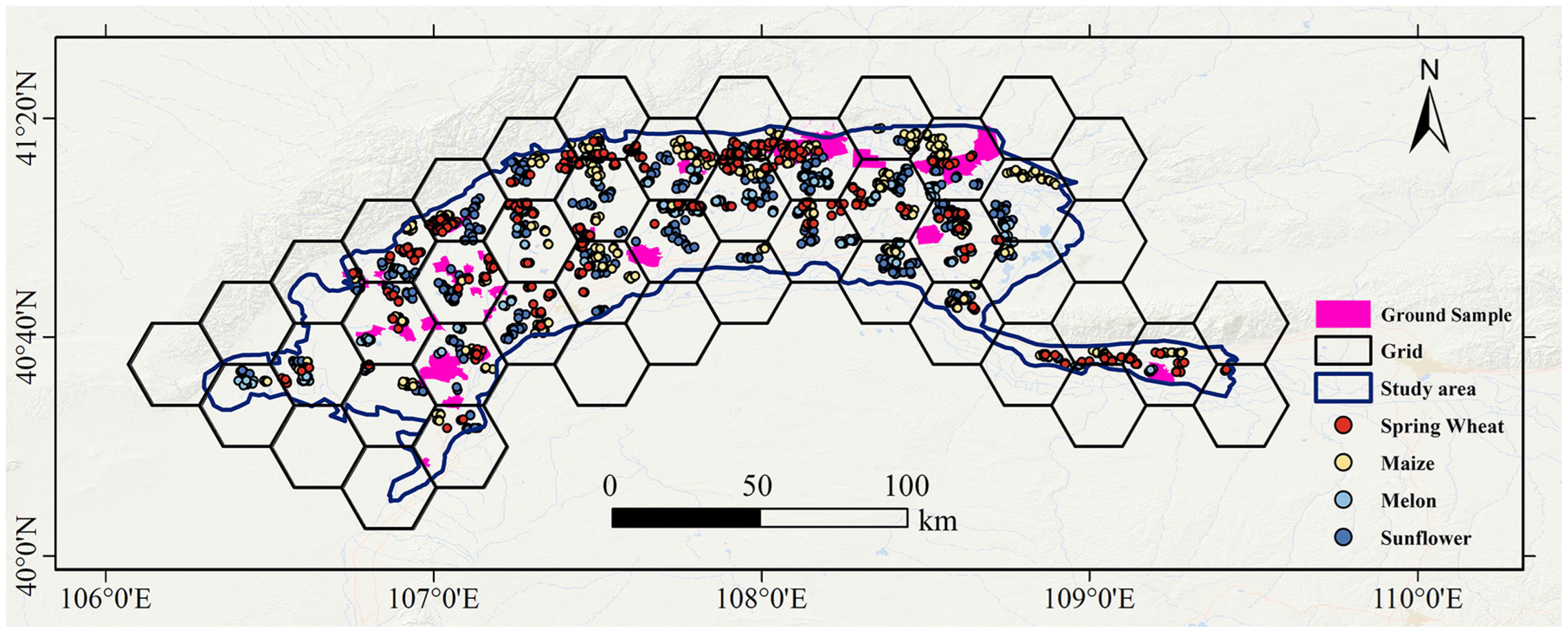
2.1. Study Area
2.2. Datasets
2.2.1. Sentinel-2
2.2.2. Sentinel-1
2.3. Reference Samples
2.4. Land Use and Land Cover Data
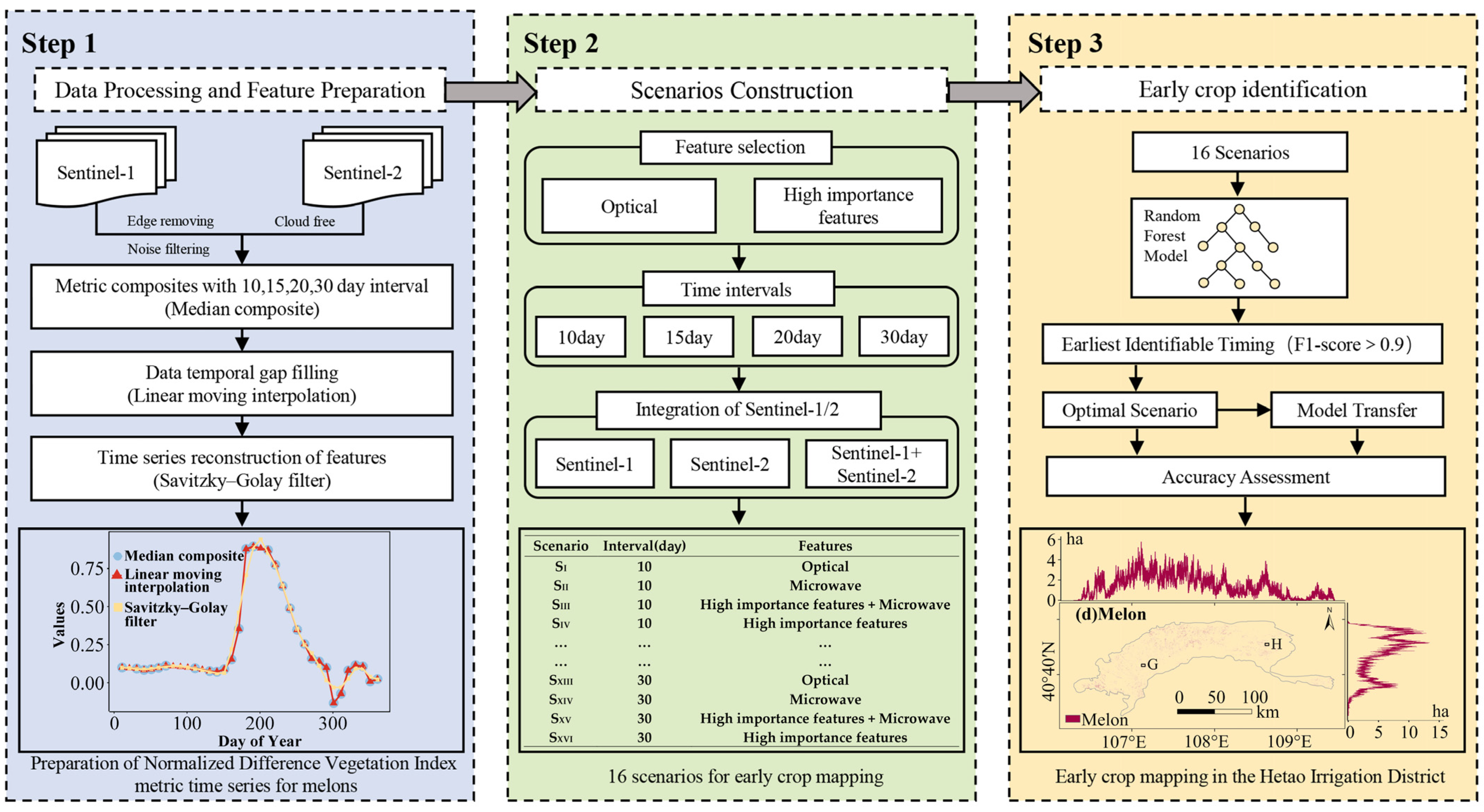
3. Methods
3.1. Data Processing and Feature Preparation
3.1.1. Data Processing
- (1)
- Sentinel-2 data processing
- (i)
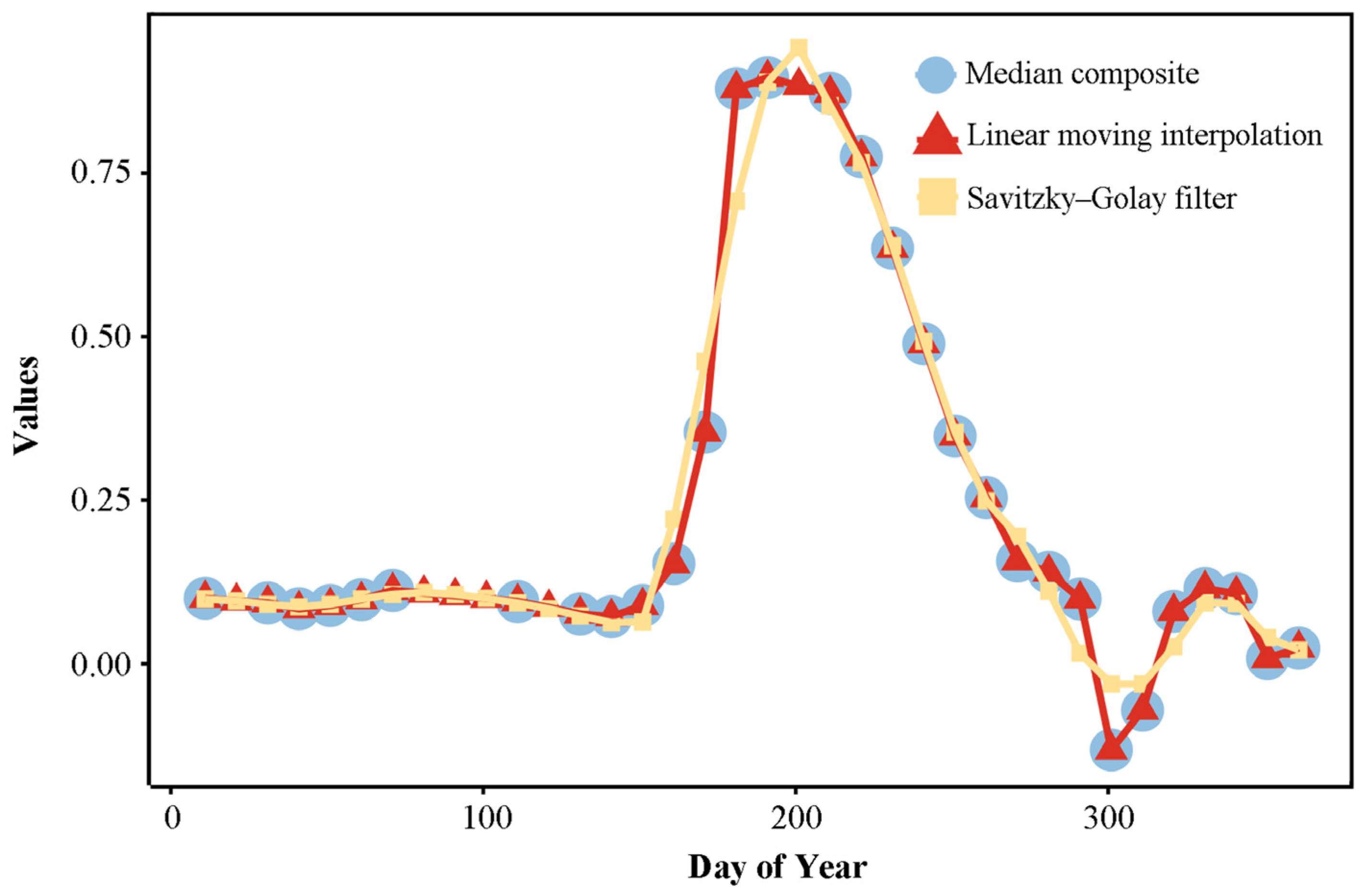
- Median synthesis was used to investigate the effect of different time intervals on early crop identification. In this paper, we synthesize the S2 feature time series with fixed time intervals of 10, 15, 20, and 30 days, covering a range from the DOY of 90 to the DOY of 300. The median synthesis method is easy to apply, and many previous studies have demonstrated its superiority over the mean synthesis method [1,41,44].
- (ii)
- Linear shift interpolation: We fill the gaps in the S2 composite time series by linear shift interpolation, which smoothes the time series of images and fills the gaps by synthetically replacing the target image with the median of three neighboring images [11,41]. This method is particularly suitable for constructing image sequences in near real-time. After analyzing the length of data gaps, we determine that the maximum missing data length is 30 days, so the window size is set to 30, and the specific formula is shown in Equation (1).
- (iii)
- SG filter. To further smooth the noise in the time series, we use an SG filter with polynomial order two and window size 3. These parameters balance the noise sensitivity and smoothing effect when processing time series data.
- (2)
- Sentinel-1 data processing
3.1.2. Feature Preparation
- (1)
- Optical remote sensing features
- (i)
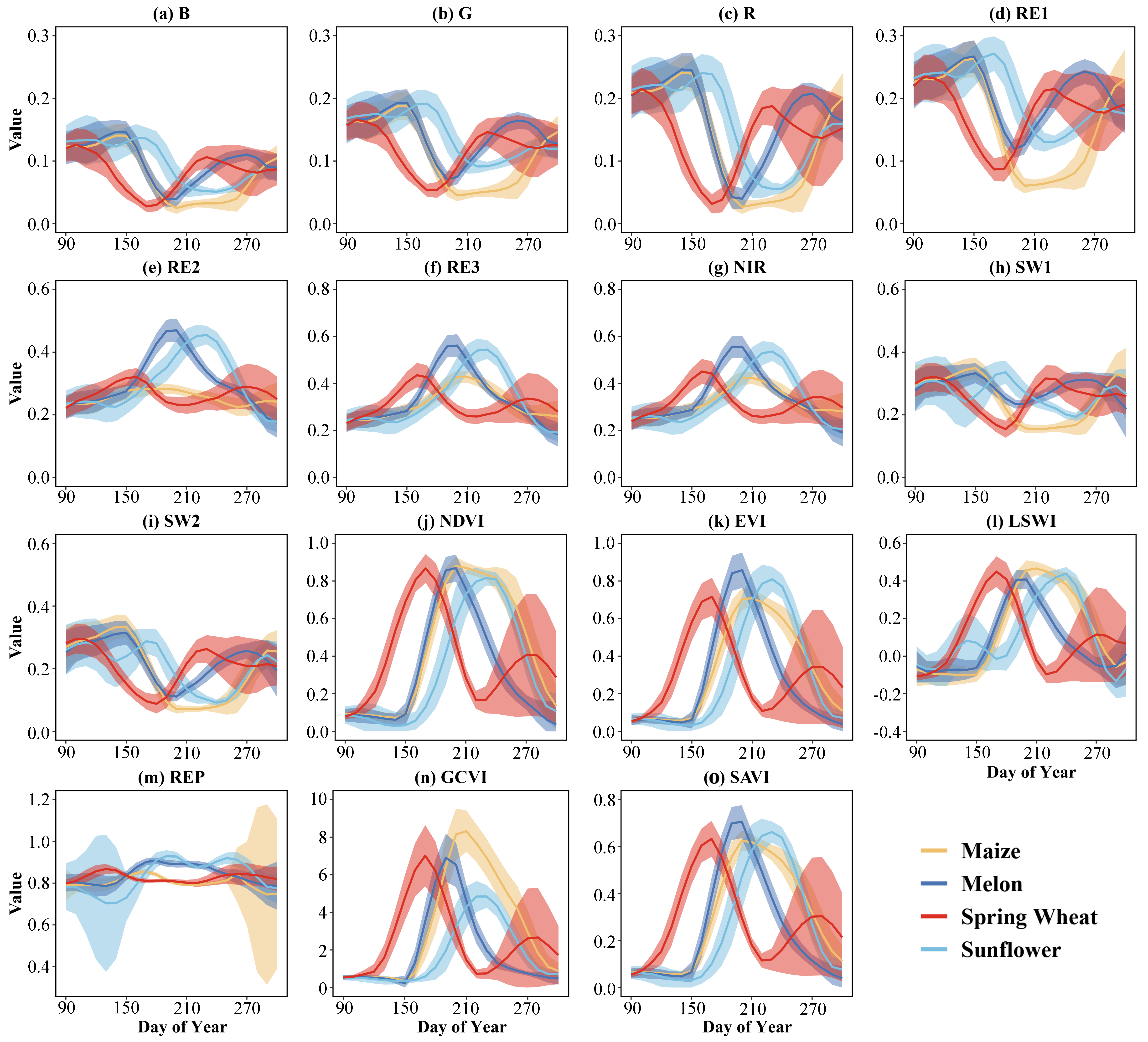
- Spectral bands. Among all 13 spectral bands, 9 spectral bands with a spatial resolution of 10 m and 20 m were used in this study as candidate features for crop identification, as shown in Table 1.
- (ii)
- Spectral indices. This study selected six spectral indices as candidate features for crop identification to improve the sensitivity of HID crop identification. NDVI is a widely used metric for identifying the distribution of crop types [46]; EVI has a solid ability to overcome the growing season saturation phenomenon [46]; LSWI is a good indicator of vegetation water content [47]; REP is a red-edge based index that is sensitive to crop conditions [48]; GCVI index has been shown to have a solid ability to separate crops [49]; SAVI is used to minimize soil background effects [46]. The specific equations used to calculate these spectral indices are shown in Table 2.
- (2)
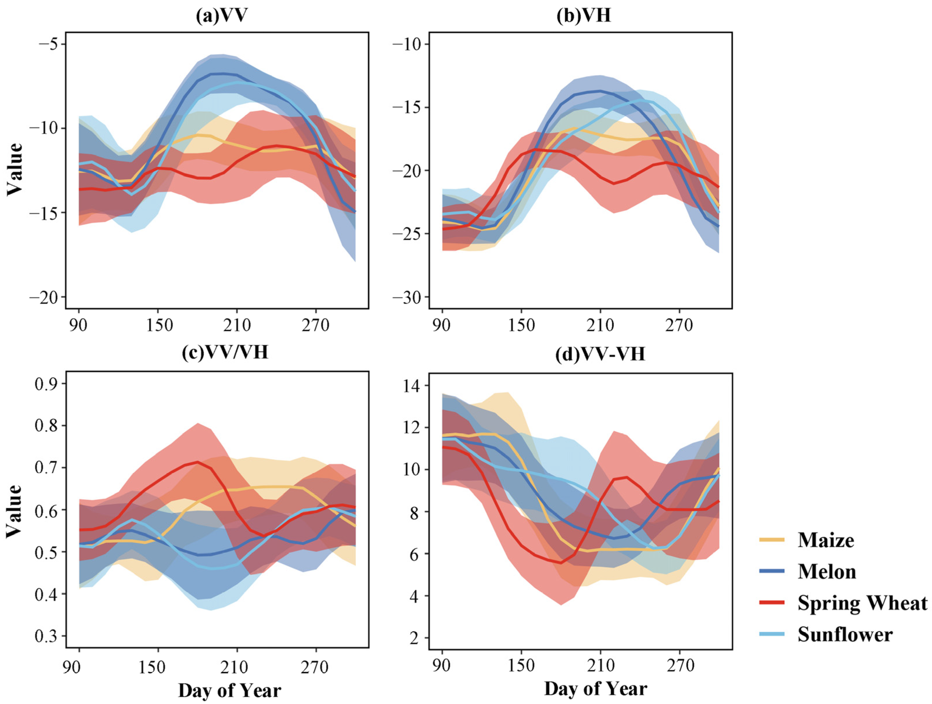
- Microwave features
3.2. Scenario Construction
3.3. Early Crop Identification
3.3.1. Random Forest Classification
3.3.2. Precision Assessment Methods
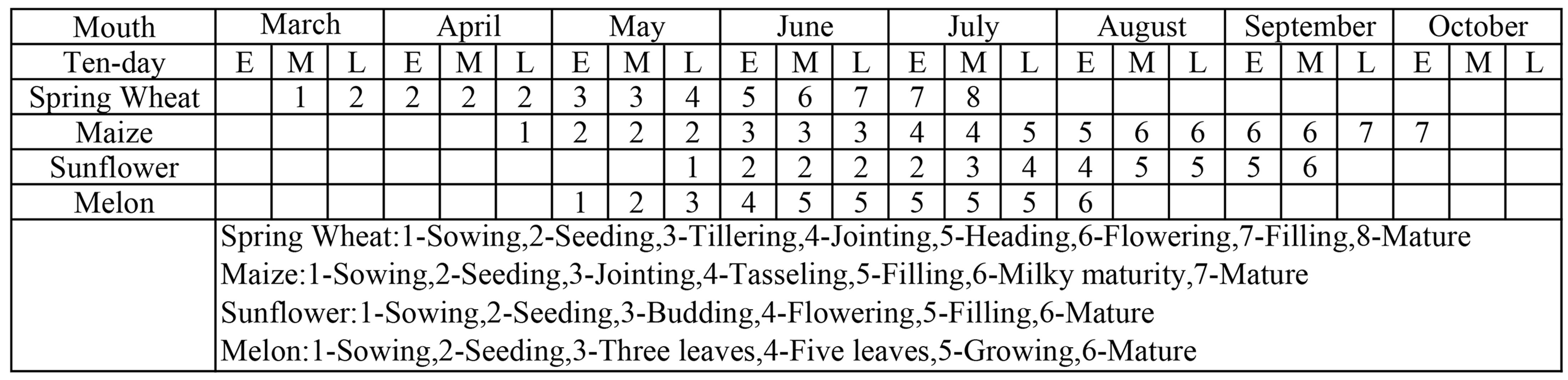
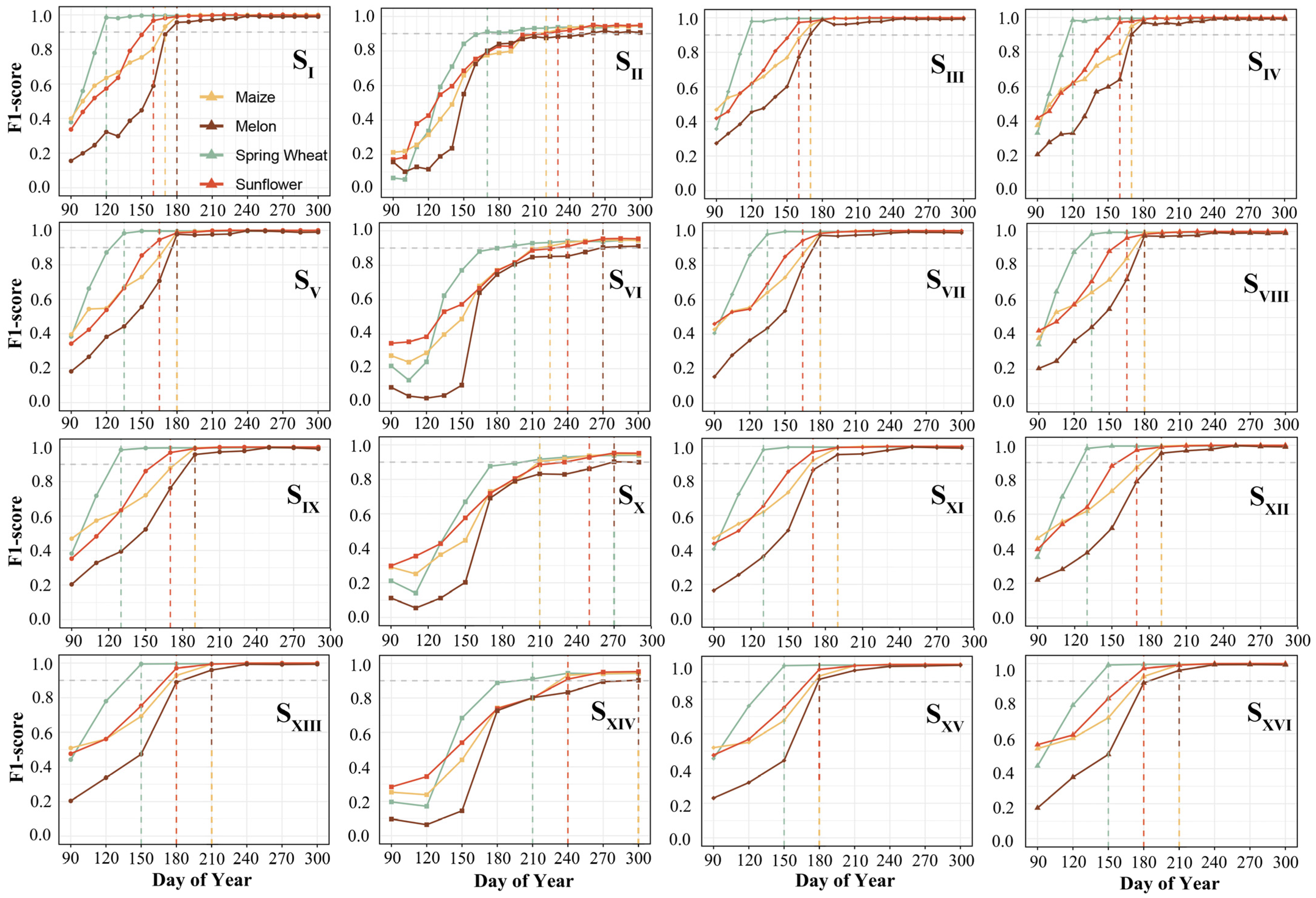
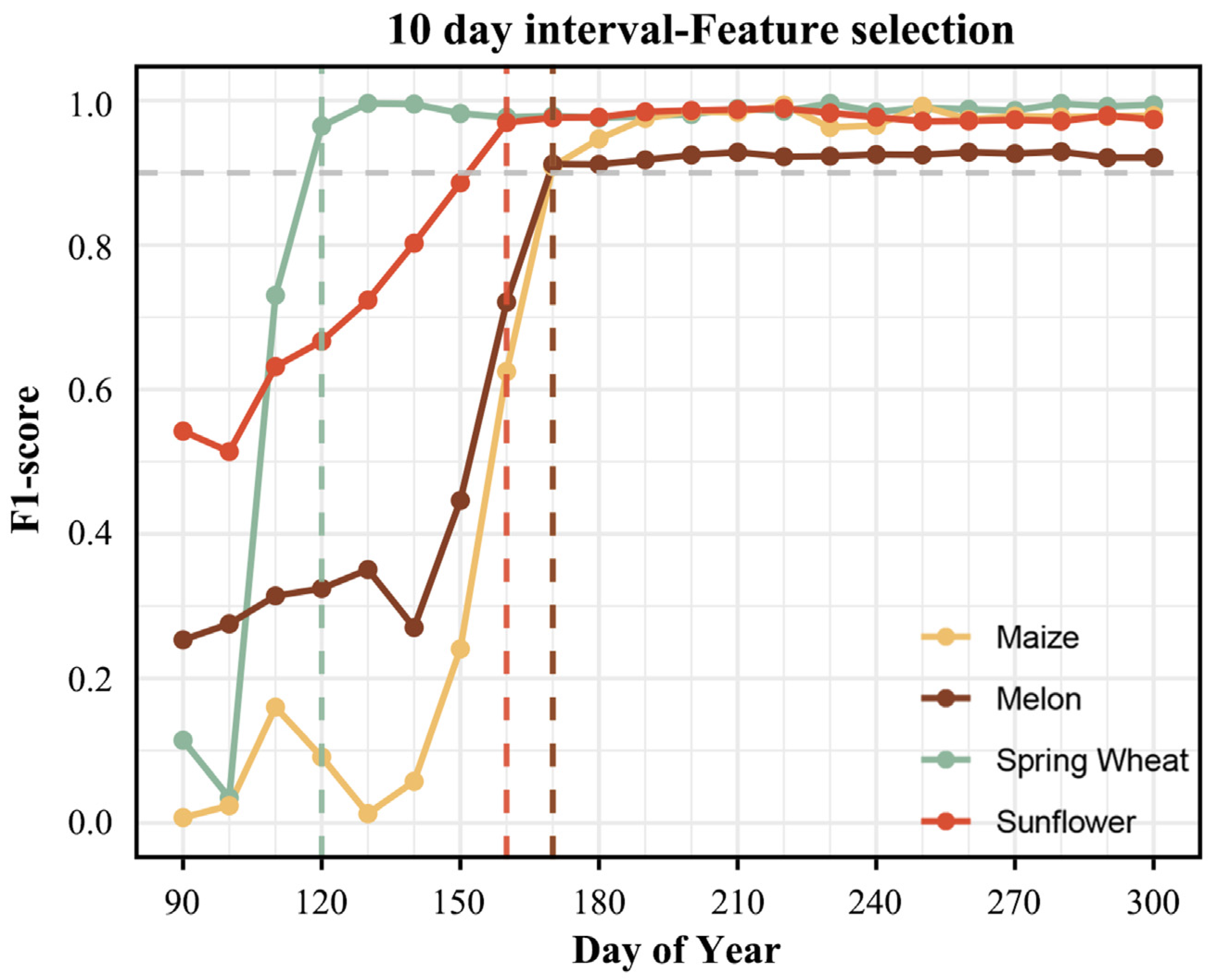
3.3.3. Determination of the Earliest Identifiable Time for Crops
3.3.4. Model Transfer
4. Results
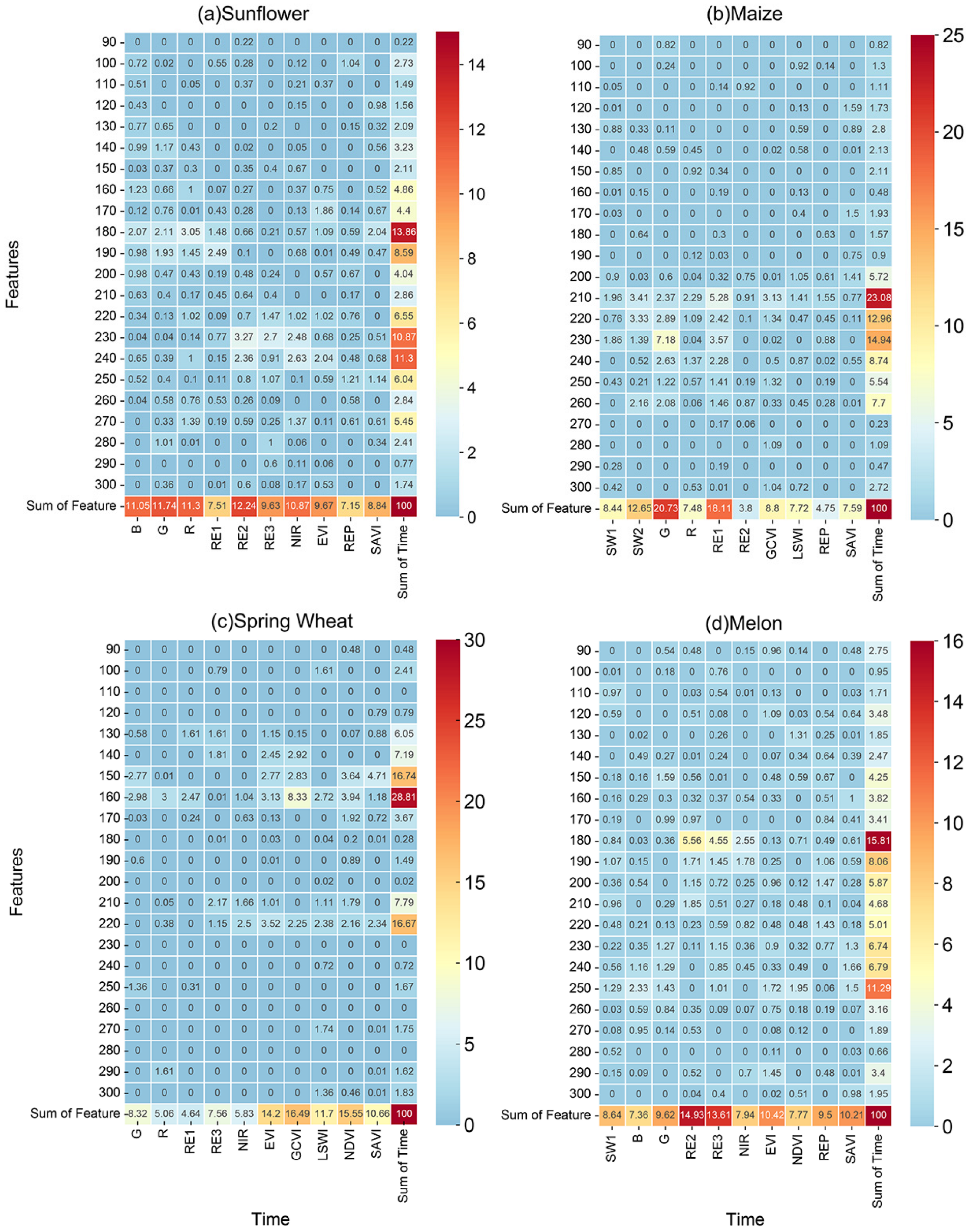
4.1. Optimal Input Characterization
4.2. Optimal Time Intervals
4.3. Optimal Data Combination
4.4. Hetao Irrigation District’s Earliest Identifiable Time for Crops
4.5. Model Transfer
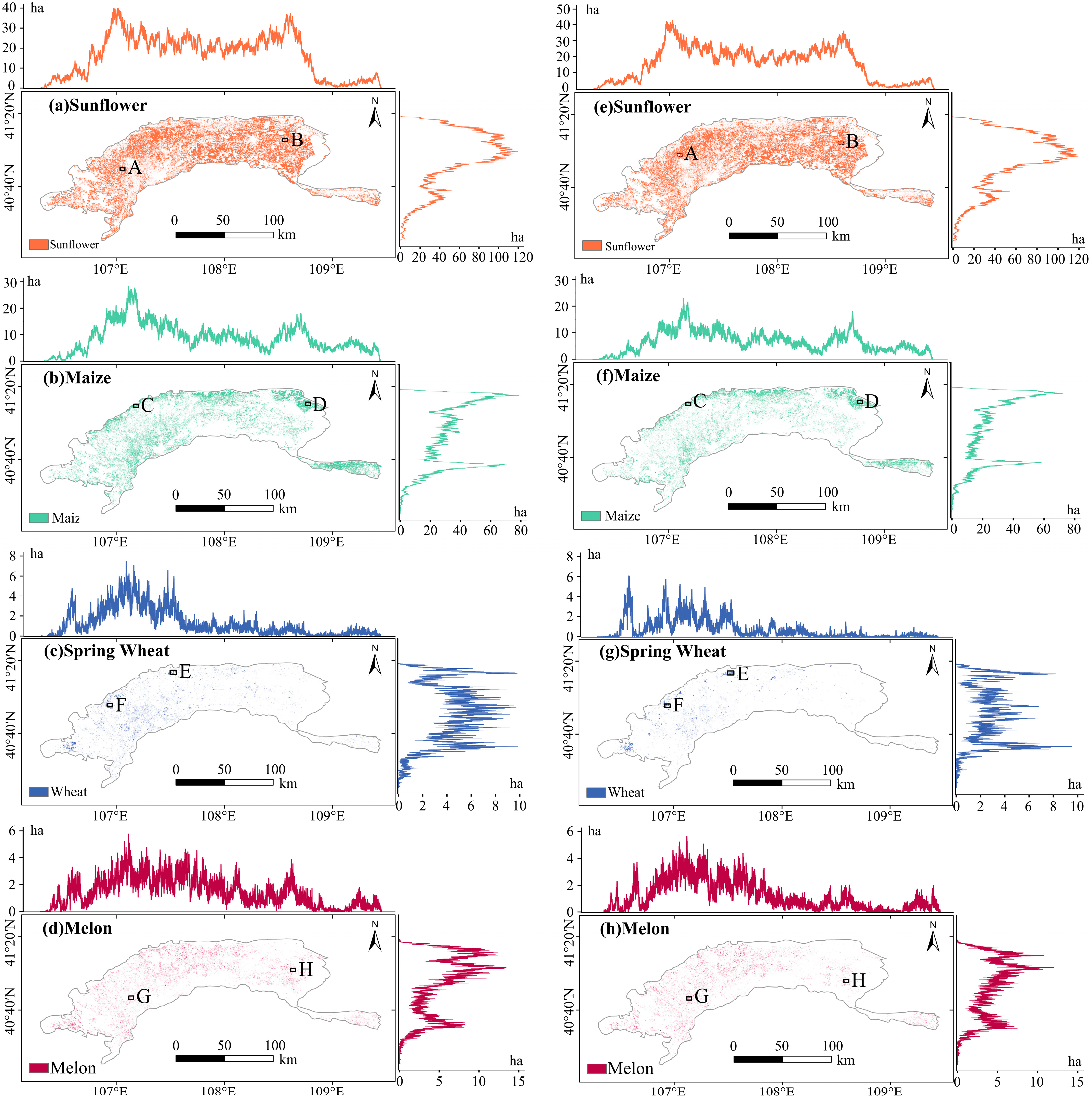
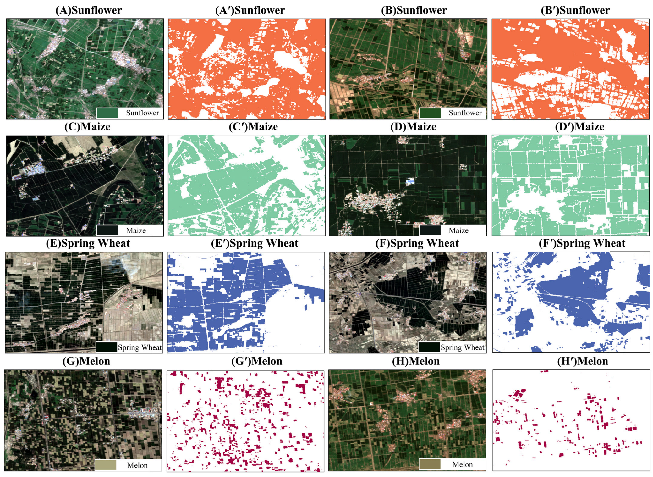
4.6. Early Season Crop Map for Hetao Irrigation District
5. Discussion
5.1. Effect of Spectral Properties
5.2. Key Identifying Features
5.3. Research Uncertainty
6. Conclusions
Author Contributions
Funding
Institutional Review Board Statement
Data Availability Statement
Acknowledgments
Conflicts of Interest
Appendix A
References
- Teluguntla, P.; Thenkabail, P.S.; Oliphant, A.; Xiong, J.; Gumma, M.K.; Congalton, R.G.; Yadav, K.; Huete, A. A 30-m landsat-derived cropland extent product of Australia and China using random forest machine learning algorithm on Google Earth Engine cloud computing platform. ISPRS J. Photogramm. Remote Sens. 2018, 144, 325–340. [Google Scholar] [CrossRef]
- Dong, J.; Fu, Y.; Wang, J.; Tian, H.; Fu, S.; Niu, Z.; Han, W.; Zheng, Y.; Huang, J.; Yuan, W. Early-season mapping of winter wheat in China based on Landsat and Sentinel images. Earth Syst. Sci. Data 2020, 12, 3081–3095. [Google Scholar] [CrossRef]
- Thenkabail, P.S.; Hanjra, M.A.; Dheeravath, V.; Gumma, M.K. A Holistic View of Global Croplands and Their Water Use for Ensuring Global Food Security in the 21st Century through Advanced Remote Sensing and Non-remote Sensing Approaches. Remote Sens. 2010, 2, 211–261. [Google Scholar] [CrossRef]
- Yi, Z.; Jia, L.; Chen, Q.; Jiang, M.; Zhou, D.; Zeng, Y. Early-Season Crop Identification in the Shiyang River Basin Using a Deep Learning Algorithm and Time-Series Sentinel-2 Data. Remote Sens. 2022, 14, 5625. [Google Scholar] [CrossRef]
- Skakun, S.; Kussul, N.; Shelestov, A.; Kussul, O. The use of satellite data for agriculture drought risk quantification in Ukraine. Geomat. Nat. Hazards Risk 2015, 7, 901–917. [Google Scholar] [CrossRef]
- Zhang, J.; Huang, Y.; Pu, R.; Gonzalez-Moreno, P.; Yuan, L.; Wu, K.; Huang, W. Monitoring plant diseases and pests through remote sensing technology: A review. Comput. Electron. Agric. 2019, 165, 104943. [Google Scholar] [CrossRef]
- Wardlow, B.D.; Callahan, K. A multi-scale accuracy assessment of the MODIS irrigated agriculture data-set (MIrAD) for the state of Nebraska, USA. Giscience Remote Sens. 2014, 51, 575–592. [Google Scholar] [CrossRef]
- Ozdogan, M.; Yang, Y.; Allez, G.; Cervantes, C. Remote Sensing of Irrigated Agriculture: Opportunities and Challenges. Remote Sens. 2010, 2, 2274–2304. [Google Scholar] [CrossRef]
- Karthikeyan, L.; Chawla, I.; Mishra, A.K. A review of remote sensing applications in agriculture for food security: Crop growth and yield, irrigation, and crop losses. J. Hydrol. 2020, 586, 124905. [Google Scholar] [CrossRef]
- Dell’acqua, F.; Iannelli, G.C.; Torres, M.A.; Martina, M.L. A Novel Strategy for Very-Large-Scale Cash-Crop Mapping in the Context of Weather-Related Risk Assessment, Combining Global Satellite Multispectral Datasets, Environmental Constraints, and In Situ Acquisition of Geospatial Data. Sensors 2018, 18, 591. [Google Scholar] [CrossRef]
- You, N.; Dong, J. Examining earliest identifiable timing of crops using all available Sentinel 1/2 imagery and Google Earth Engine. ISPRS J. Photogramm. Remote Sens. 2020, 161, 109–123. [Google Scholar] [CrossRef]
- Wei, M.; Wang, H.; Zhang, Y.; Li, Q.; Du, X.; Shi, G.; Ren, Y. Investigating the Potential of Sentinel-2 MSI in Early Crop Identification in Northeast China. Remote Sens. 2022, 14, 1928. [Google Scholar] [CrossRef]
- You, N.; Dong, J.; Li, J.; Huang, J.; Jin, Z. Rapid early-season maize mapping without crop labels. Remote Sens. Environ. 2023, 290, 113496. [Google Scholar] [CrossRef]
- Vorobiova, N.S.; Chernov, A.V. Curve fitting of MODIS NDVI time series in the task of early crops identification by satellite images. Procedia Eng. 2017, 201, 184–195. [Google Scholar] [CrossRef]
- Jordi, I.; Arthur, V.; Marcela, A.; Claire, M.-S. Improved Early Crop Type Identification By Joint Use of High Temporal Resolution SAR And Optical Image Time Series. Remote Sens. 2016, 8, 362. [Google Scholar] [CrossRef]
- Li, G.; Cui, J.; Han, W.; Zhang, H.; Huang, S.; Chen, H.; Ao, J. Crop type mapping using time-series Sentinel-2 imagery and U-Net in early growth periods in the Hetao irrigation district in China. Comput. Electron. Agric. 2022, 203, 107478. [Google Scholar] [CrossRef]
- Huang, X.; Huang, J.; Li, X.; Shen, Q.; Chen, Z. Early mapping of winter wheat in Henan province of China using time series of Sentinel-2 data. GIScience Remote Sens. 2022, 59, 1534–1549. [Google Scholar] [CrossRef]
- Khan, H.R.; Gillani, Z.; Jamal, M.H.; Athar, A.; Chaudhry, M.T.; Chao, H.; He, Y.; Chen, M. Early Identification of Crop Type for Smallholder Farming Systems Using Deep Learning on Time-Series Sentinel-2 Imagery. Sensors 2023, 23, 1779. [Google Scholar] [CrossRef]
- Valero, S.; Arnaud, L.; Planells, M.; Ceschia, E. Synergy of Sentinel-1 and Sentinel-2 Imagery for Early Seasonal Agricultural Crop Mapping. Remote Sens. 2021, 13, 4891. [Google Scholar] [CrossRef]
- El Imanni, H.S.; El Harti, A.; Hssaisoune, M.; Velastegui-Montoya, A.; Elbouzidi, A.; Addi, M.; El Iysaouy, L.; El Hachimi, J. Rapid and Automated Approach for Early Crop Mapping Using Sentinel-1 and Sentinel-2 on Google Earth Engine; A Case of a Highly Heterogeneous and Fragmented Agricultural Region. J. Imaging 2022, 8, 316. [Google Scholar] [CrossRef]
- Paul, S.; Kumari, M.; Murthy, C.S.; Kumar, D.N. Generating pre-harvest crop maps by applying convolutional neural network on multi-temporal Sentinel-1 data. Int. J. Remote Sens. 2022, 43, 6078–6101. [Google Scholar] [CrossRef]
- Hao, P.-Y.; Tang, H.-J.; Chen, Z.-X.; Meng, Q.-Y.; Kang, Y.-P. Early-season crop type mapping using 30-m reference time series. J. Integr. Agric. 2020, 19, 1897–1911. [Google Scholar] [CrossRef]
- Tian, H.; Wang, Y.; Chen, T.; Zhang, L.; Qin, Y. Early-Season Mapping of Winter Crops Using Sentinel-2 Optical Imagery. Remote Sens. 2021, 13, 3822. [Google Scholar] [CrossRef]
- Li, G.; Han, W.; Dong, Y.; Zhai, X.; Huang, S.; Ma, W.; Cui, X.; Wang, Y. Multi-Year Crop Type Mapping Using Sentinel-2 Imagery and Deep Semantic Segmentation Algorithm in the Hetao Irrigation District in China. Remote Sens. 2023, 15, 875. [Google Scholar] [CrossRef]
- Domínguez, J.; Kumhálová, J.; Novák, P. Winter oilseed rape and winter wheat growth prediction using remote sensing methods. Plant Soil Environ. 2015, 61, 410–416. [Google Scholar] [CrossRef]
- Narin, O.G.; Abdikan, S. Monitoring of phenological stage and yield estimation of sunflower plant using Sentinel-2 satellite images. Geocarto Int. 2020, 37, 1378–1392. [Google Scholar] [CrossRef]
- Qiu, B.; Hu, X.; Yang, P.; Tang, Z.; Wu, W.; Li, Z. A robust approach for large-scale cropping intensity mapping in smallholder farms from vegetation, brownness indices and SAR time series. ISPRS J. Photogramm. Remote Sens. 2023, 203, 328–344. [Google Scholar] [CrossRef]
- Yu, B.; Shang, S. Multi-Year Mapping of Maize and Sunflower in Hetao Irrigation District of China with High Spatial and Temporal Resolution Vegetation Index Series. Remote Sens. 2017, 9, 855. [Google Scholar] [CrossRef]
- Bing, Y.; Songhao, S.; Wenxiang, Z.; Pierre, G.; Yizong, C. Mapping daily evapotranspiration over a large irrigation district from MODIS data using a novel hybrid dual-source coupling model. Agric. For. Meteorol. 2019, 276–277, 107612. [Google Scholar] [CrossRef]
- Karra, K.; Kontgis, C.; Statman-Weil, Z.; Mazzariello, J.C.; Mathis, M.; Brumby, S.P. Global land use/land cover with Sentinel 2 and deep learning. In Proceedings of the 2021 IEEE International Geoscience and Remote Sensing Symposium IGARSS, Brussels, Belgium, 11–16 July 2021. [Google Scholar] [CrossRef]
- Liu, J.; Sun, S.; Wu, P.; Wang, Y.; Zhao, X. Inter-county virtual water flows of the Hetao irrigation district, China: A new perspective for water scarcity. J. Arid. Environ. 2015, 119, 31–40. [Google Scholar] [CrossRef]
- Zhang, X.; Guo, P.; Zhang, F.; Liu, X.; Yue, Q.; Wang, Y. Optimal irrigation water allocation in Hetao Irrigation District considering decision makers’ preference under uncertainties. Agric. Water Manag. 2020, 246, 106670. [Google Scholar] [CrossRef]
- Hu, Y.; Zeng, H.; Tian, F.; Zhang, M.; Wu, B.; Gilliams, S.; Li, S.; Li, Y.; Lu, Y.; Yang, H. An Interannual Transfer Learning Approach for Crop Classification in the Hetao Irrigation District, China. Remote Sens. 2022, 14, 1208. [Google Scholar] [CrossRef]
- Drusch, M.; Del Bello, U.; Carlier, S.; Colin, O.; Fernandez, V.; Gascon, F.; Hoersch, B.; Isola, C.; Laberinti, P.; Martimort, P.; et al. Sentinel-2: ESA’s Optical High-Resolution Mission for GMES Operational Services. Remote Sens. Environ. 2012, 120, 25–36. [Google Scholar] [CrossRef]
- Tuvdendorj, B.; Zeng, H.; Wu, B.; Elnashar, A.; Zhang, M.; Tian, F.; Nabil, M.; Nanzad, L.; Bulkhbai, A.; Natsagdorj, N. Performance and the Optimal Integration of Sentinel-1/2 Time-Series Features for Crop Classification in Northern Mongolia. Remote Sens. 2022, 14, 1830. [Google Scholar] [CrossRef]
- Xun, L.; Zhang, J.; Cao, D.; Yang, S.; Yao, F. A novel cotton mapping index combining Sentinel-1 SAR and Sentinel-2 multispectral imagery. ISPRS J. Photogramm. Remote Sens. 2021, 181, 148–166. [Google Scholar] [CrossRef]
- D’andrimont, R.; Verhegghen, A.; Lemoine, G.; Kempeneers, P.; Meroni, M.; van der Velde, M. From parcel to continental scale—A first European crop type map based on Sentinel-1 and LUCAS Copernicus in-situ observations. Remote Sens. Environ. 2021, 266, 112708. [Google Scholar] [CrossRef]
- Zhang, X.; Wu, B.; Ponce-Campos, G.E.; Zhang, M.; Chang, S.; Tian, F. Mapping up-to-Date Paddy Rice Extent at 10 M Resolution in China through the Integration of Optical and Synthetic Aperture Radar Images. Remote Sens. 2018, 10, 1200. [Google Scholar] [CrossRef]
- Xiao, W.; Xu, S.; He, T. Mapping Paddy Rice with Sentinel-1/2 and Phenology-, Object-Based Algorithm—A Implementation in Hangjiahu Plain in China Using GEE Platform. Remote Sens. 2021, 13, 990. [Google Scholar] [CrossRef]
- Liu, W.; Zhang, H. Mapping annual 10 m rapeseed extent using multisource data in the Yangtze River Economic Belt of China (2017–2021) on Google Earth Engine. Int. J. Appl. Earth Obs. Geoinf. 2023, 117, 103198. [Google Scholar] [CrossRef]
- Griffiths, P.; Nendel, C.; Hostert, P. Intra-annual reflectance composites from Sentinel-2 and Landsat for national-scale crop and land cover mapping. Remote Sens. Environ. 2019, 220, 135–151. [Google Scholar] [CrossRef]
- Tran, K.H.; Zhang, H.K.; McMaine, J.T.; Zhang, X.; Luo, D. 10 m crop type mapping using Sentinel-2 reflectance and 30 m cropland data layer product. Int. J. Appl. Earth Obs. Geoinf. 2022, 107, 102692. [Google Scholar] [CrossRef]
- Chen, J.; Jönsson, P.; Tamura, M.; Gu, Z.; Matsushita, B.; Eklundh, L. A simple method for reconstructing a high-quality NDVI time-series data set based on the Savitzky–Golay filter. Remote Sens. Environ. 2004, 91, 332–344. [Google Scholar] [CrossRef]
- Roy, D.P.; Wulder, M.A.; Loveland, T.R.; Woodcock, C.E.; Allen, R.G.; Anderson, M.C.; Helder, D.; Irons, J.R.; Johnson, D.M.; Kennedy, R.; et al. Landsat-8: Science and product vision for terrestrial global change research. Remote Sens. Environ. 2014, 145, 154–172. [Google Scholar] [CrossRef]
- Lee, J.-S. Refined filtering of image noise using local statistics. Comput. Graph. Image Process. 1981, 15, 380–389. [Google Scholar] [CrossRef]
- Huete, A.; Didan, K.; Miura, T.; Rodriguez, E.P.; Gao, X.; Ferreira, L.G. Overview of the radiometric and biophysical performance of the MODIS vegetation indices. Remote Sens. Environ. 2002, 83, 195–213. [Google Scholar] [CrossRef]
- Yin, L.; You, N.; Zhang, G.; Huang, J.; Dong, J. Optimizing Feature Selection of Individual Crop Types for Improved Crop Mapping. Remote Sens. 2020, 12, 162. [Google Scholar] [CrossRef]
- Frampton, W.J.; Dash, J.; Watmough, G.; Milton, E.J. Evaluating the capabilities of Sentinel-2 for quantitative estimation of biophysical variables in vegetation. ISPRS J. Photogramm. Remote Sens. 2013, 82, 83–92. [Google Scholar] [CrossRef]
- Gitelson, A.A.; Viña, A.; Ciganda, V.; Rundquist, D.C.; Arkebauer, T.J. Remote estimation of canopy chlorophyll content in crops. Geophys. Res. Lett. 2005, 32, L08403. [Google Scholar] [CrossRef]
- Veloso, A.; Mermoz, S.; Bouvet, A.; Le Toan, T.; Planells, M.; Dejoux, J.-F.; Ceschia, E. Understanding the temporal behavior of crops using Sentinel-1 and Sentinel-2-like data for agricultural applications. Remote Sens. Environ. 2017, 199, 415–426. [Google Scholar] [CrossRef]
- Breiman, L. Random Forests. Mach. Learn. 2001, 45, 5–32. [Google Scholar] [CrossRef]
- Rodriguez-Galiano, V.F.; Ghimire, B.; Rogan, J.; Chica-Olmo, M.; Rigol-Sanchez, J.P. An assessment of the effectiveness of a random forest classifier for land-cover classification. ISPRS J. Photogramm. Remote Sens. 2012, 67, 93–104. [Google Scholar] [CrossRef]
- Maxwell, A.E.; Warner, T.A.; Fang, F. Implementation of machine-learning classification in remote sensing: An applied review. Int. J. Remote Sens. 2018, 39, 2784–2817. [Google Scholar] [CrossRef]
- Zhang, L.; Tang, H.; Shi, P.; Jia, W.; Dai, L. Geographically and Ontologically Oriented Scoping of a Dry Valley and Its Spatial Characteristics Analysis: The Case of the Three Parallel Rivers Region. Land 2023, 12, 1235. [Google Scholar] [CrossRef]
- Luo, J.; Ma, X.; Chu, Q.; Xie, M.; Cao, Y. Characterizing the Up-To-Date Land-Use and Land-Cover Change in Xiong’an New Area from 2017 to 2020 Using the Multi-Temporal Sentinel-2 Images on Google Earth Engine. ISPRS Int. J. Geo-Inf. 2021, 10, 464. [Google Scholar] [CrossRef]
- Pelletier, C.; Valero, S.; Inglada, J.; Champion, N.; Dedieu, G. Assessing the robustness of Random Forests to map land cover with high resolution satellite image time series over large areas. Remote Sens. Environ. 2016, 187, 156–168. [Google Scholar] [CrossRef]
- Congalton, R.G.; Green, K. Assessing the Accuracy of Remotely Sensed Data; CRC Press: Boca Raton, FL, USA, 2019. [Google Scholar] [CrossRef]
- Carrão, H.; Gonçalves, P.; Caetano, M. Contribution of multispectral and multitemporal information from MODIS images to land cover classification. Remote Sens. Environ. 2008, 112, 986–997. [Google Scholar] [CrossRef]
- Löw, F.; Michel, U.; Dech, S.; Conrad, C. Impact of feature selection on the accuracy and spatial uncertainty of per-field crop classification using Support Vector Machines. ISPRS J. Photogramm. Remote Sens. 2013, 85, 102–119. [Google Scholar] [CrossRef]
- Adrian, J.; Sagan, V.; Maimaitijiang, M. Sentinel SAR-optical fusion for crop type mapping using deep learning and Google Earth Engine. ISPRS J. Photogramm. Remote Sens. 2021, 175, 215–235. [Google Scholar] [CrossRef]
- Van Tricht, K.; Gobin, A.; Gilliams, S.; Piccard, I. Synergistic Use of Radar Sentinel-1 and Optical Sentinel-2 Imagery for Crop Mapping: A Case Study for Belgium. Remote Sens. 2018, 10, 1642. [Google Scholar] [CrossRef]
- Forkuor, G.; Conrad, C.; Thiel, M.; Ullmann, T.; Zoungrana, E. Integration of Optical and Synthetic Aperture Radar Imagery for Improving Crop Mapping in Northwestern Benin, West Africa. Remote Sens. 2014, 6, 6472–6499. [Google Scholar] [CrossRef]
- Debaeke, P.; Attia, F.; Champolivier, L.; Dejoux, J.-F.; Micheneau, A.; Al Bitar, A.; Trépos, R. Forecasting sunflower grain yield using remote sensing data and statistical models. Eur. J. Agron. 2023, 142, 126677. [Google Scholar] [CrossRef]
- Nieto, L.; Schwalbert, R.; Prasad, P.V.V.; Olson, B.J.S.C.; Ciampitti, I.A. An integrated approach of field, weather, and satellite data for monitoring maize phenology. Sci. Rep. 2021, 11, 15711. [Google Scholar] [CrossRef]
- Zhang, L.; Zhang, Z.; Luo, Y.; Cao, J.; Xie, R.; Li, S. Integrating satellite-derived climatic and vegetation indices to predict smallholder maize yield using deep learning. Agric. For. Meteorol. 2021, 311, 108666. [Google Scholar] [CrossRef]
- Liu, S.; Peng, D.; Zhang, B.; Chen, Z.; Yu, L.; Chen, J.; Pan, Y.; Zheng, S.; Hu, J.; Lou, Z.; et al. The Accuracy of Winter Wheat Identification at Different Growth Stages Using Remote Sensing. Remote Sens. 2022, 14, 893. [Google Scholar] [CrossRef]
- Fan, L.; Yang, J.; Sun, X.; Zhao, F.; Liang, S.; Duan, D.; Chen, H.; Xia, L.; Sun, J.; Yang, P. The effects of Landsat image acquisition date on winter wheat classification in the North China Plain. ISPRS J. Photogramm. Remote Sens. 2022, 187, 1–13. [Google Scholar] [CrossRef]
- Li, S.; Li, F.; Gao, M.; Li, Z.; Leng, P.; Duan, S.; Ren, J. A New Method for Winter Wheat Mapping Based on Spectral Reconstruction Technology. Remote Sens. 2021, 13, 1810. [Google Scholar] [CrossRef]
- Pan, L.; Xia, H.; Zhao, X.; Guo, Y.; Qin, Y. Mapping Winter Crops Using a Phenology Algorithm, Time-Series Sentinel-2 and Landsat-7/8 Images, and Google Earth Engine. Remote Sens. 2021, 13, 2510. [Google Scholar] [CrossRef]
- Yin, H.; Prishchepov, A.V.; Kuemmerle, T.; Bleyhl, B.; Buchner, J.; Radeloff, V.C. Mapping agricultural land abandonment from spatial and temporal segmentation of Landsat time series. Remote Sens. Environ. 2018, 210, 12–24. [Google Scholar] [CrossRef]
- Račič, M.; Oštir, K.; Zupanc, A.; Zajc, L.Č. Multi-Year Time Series Transfer Learning: Application of Early Crop Classification. Remote Sens. 2024, 16, 270. [Google Scholar] [CrossRef]
- Gadiraju, K.K.; Vatsavai, R.R. Remote Sensing Based Crop Type Classification Via Deep Transfer Learning. IEEE J. Sel. Top. Appl. Earth Obs. Remote Sens. 2023, 16, 4699–4712. [Google Scholar] [CrossRef]
- Munipalle, V.K.; Nelakuditi, U.R.; Nidamanuri, R.R. Agricultural Crop Hyperspectral Image Classification using Transfer Learning. In Proceedings of the 2023 International Conference on Machine Intelligence for GeoAnalytics and Remote Sensing (MIGARS), Hyderabad, India, 27–29 January 2023. [Google Scholar] [CrossRef]
- Osman, M.A.A.; Onono, J.O.; Olaka, L.A.; Elhag, M.M.; Abdel-Rahman, E.M. Climate Variability and Change Affect Crops Yield under Rainfed Conditions: A Case Study in Gedaref State, Sudan. Agronomy 2021, 11, 1680. [Google Scholar] [CrossRef]
- He, L.; Jin, N.; Yu, Q. Impacts of climate change and crop management practices on soybean phenology changes in China. Sci. Total. Environ. 2019, 707, 135638. [Google Scholar] [CrossRef]
- Ozelkan, E.; Chen, G.; Ustundag, B.B. Multiscale object-based drought monitoring and comparison in rainfed and irrigated agriculture from Landsat 8 OLI imagery. Int. J. Appl. Earth Obs. Geoinf. 2016, 44, 159–170. [Google Scholar] [CrossRef]
- Cai, Y.; Guan, K.; Peng, J.; Wang, S.; Seifert, C.; Wardlow, B.; Li, Z. A high-performance and in-season classification system of field-level crop types using time-series Landsat data and a machine learning approach. Remote Sens. Environ. 2018, 210, 35–47. [Google Scholar] [CrossRef]
- Wang, S.; Azzari, G.; Lobell, D.B. Crop type mapping without field-level labels: Random forest transfer and unsupervised clustering techniques. Remote Sens. Environ. 2019, 222, 303–317. [Google Scholar] [CrossRef]
- Das, T.; Jana, A.; Mandal, B.; Sutradhar, A. Spatio-temporal pattern of land use and land cover and its effects on land surface temperature using remote sensing and GIS techniques: A case study of Bhubaneswar city, Eastern India (1991–2021). GeoJournal 2021, 87, 765–795. [Google Scholar] [CrossRef]
- Fathololoumi, S.; Firozjaei, M.K.; Biswas, A. An Innovative Fusion-Based Scenario for Improving Land Crop Mapping Accuracy. Sensors 2022, 22, 7428. [Google Scholar] [CrossRef]

| Band No | Band Type | Central Wavelength/nm | Spatial Resolution/m | Abbreviation Used in This Study |
|---|---|---|---|---|
| B2 | Blue | 490 | 10 | B |
| B3 | Green | 560 | 10 | G |
| B4 | Red | 665 | 10 | R |
| B5 | Vegetation Red Edge 1 | 705 | 20 | RE1 |
| B6 | Vegetation Red Edge 2 | 740 | 20 | RE2 |
| B7 | Vegetation Red Edge 3 | 783 | 20 | RE3 |
| B8 | Near-infrared | 842 | 10 | NIR |
| B11 | Shortwave infrared 1 | 1610 | 20 | SW1 |
| B12 | Shortwave infrared 2 | 2190 | 20 | SW2 |
| Spectral Index | Expression Using Sentinel-2 Bands | References | Physical Meanings |
|---|---|---|---|
| NDVI | (B8 − B4)/(B8 + B4) | Huete et al. (2002) [46] | Reflective information, such as crop growth trends and health status of different vegetation cover |
| EVI | 2.5 × (B8 − B4)/(B8 + 6 × B4 − 7.5 × B2 + 1) | Huete et al. (2002) [46] | It uses a blue light band that helps suppress atmospheric, background, and soil effects. |
| LSWI | (B8 − B11)/(B8 + B11) | Yin et al. (2020) [47] | Sensitive to water content and can effectively characterize soil and canopy water content in different vegetation |
| REP | 705 + 35 × (((B4 + B7)/2) − B5)/(B6 − B5) | Frampton et al. (2013) [48] | For assessing the extent of vegetation cover |
| GCVI | (B4/B2) − 1 | Gitelson et al. (2005) [49] | Describes the image synthetic activity of vegetation |
| SAVI | 1.5 × (B8 − B4)/(B8 + B4 + 0.5) | Huete et al. (2002) [46] | Interpretation of changes in the optical characteristics of the background and correction of the sensitivity of NDVI to the soil background |
| Scenario | Interval (day) | Features |
|---|---|---|
| SI | 10 | Optical |
| SII | 10 | Microwave |
| SIII | 10 | High importance features + Microwave |
| SIV | 10 | High importance features |
| SV | 15 | Optical |
| SVI | 15 | Microwave |
| SVII | 15 | High importance features + Microwave |
| SVIII | 15 | High importance features |
| SIX | 20 | Optical |
| SX | 20 | Microwave |
| SXI | 20 | High importance features + Microwave |
| SXII | 20 | High importance features |
| SXIII | 30 | Optical |
| SXIV | 30 | Microwave |
| SXV | 30 | High importance features + Microwave |
| SXVI | 30 | High importance features |
| Time Interval (Day) | Crop Types | Feature Selection | Score |
|---|---|---|---|
| 10 | Sunflower | RE2, NIR, RE1, G, EVI, R, RE3, SAVI, REP and B | 79.84 |
| Maize | RE1, SW1, R, SW2, G, REP, GCVI, LSWI, SAVI and RE2 | 87.49 | |
| Spring Wheat | NDVI, EVI, SAVI, R, GCVI, RE2, G, LSWI, NIR and RE1 | 89.11 | |
| Melon | REP, RE2, EVI, SAVI, B, NIR, G, SW1, NDVI and RE3 | 75.73 | |
| 15 | Sunflower | RE3, REP, R, RE2, GCVI, G, NIR, RE1, SAVI and SW2 | 75.03 |
| Maize | G, RE1, B, GCVI, SW1, R, SW2, NIR, NDVI and REP | 82.59 | |
| Spring Wheat | NDVI, SAVI, GCVI, LSWI, R, EVI, SW2, RE3, B and SW1 | 87.57 | |
| Melon | RE2, LSWI, REP, RE3, NIR, G, EVI, SW2, RE1 and GCVI | 77.32 | |
| 20 | Sunflower | RE2, REP, RE3, RE1, NDVI, SW2, R, B, NIR and EVI | 75.21 |
| Maize | RE1, G, SW2, SW1, B, LSWI, REP, R, GCVI and EVI | 81.38 | |
| Spring Wheat | NDVI, EVI, G, RE1, SAVI, LSWI, RE3, NIR, GCVI and B | 81.41 | |
| Melon | RE2, RE1, SAVI, NIR, SW2, EVI, REP, LSWI, RE3 and NDVI | 75.07 | |
| 30 | Sunflower | RE2, NIR, RE3, EVI, NDVI, GCVI, REP, B, G and RE1 | 75.66 |
| Maize | B, RE1, REP, G, EVI, GCVI, R, SW1, NIR and SW2 | 81.85 | |
| Spring Wheat | SAVI, LSWI, RE3, G, EVI, NDVI, B, NIR, SW2 and GCVI | 83.05 | |
| Melon | RE2, G, SAVI, SW1, RE1, EVI, SW2, RE3, REP and LSWI | 75.52 |
| Categories | 2021 | 2022 |
|---|---|---|
| Sunflower | 43.73 (52.2%) | 45.06 (53.8%) |
| Maize | 26.63 (31.8%) | 25.88 (30.9%) |
| Spring Wheat | 3.33 (4%) | 3.18 (3.8%) |
| Melon | 3.76 (4.5%) | 3.52 (4.2%) |
Disclaimer/Publisher’s Note: The statements, opinions and data contained in all publications are solely those of the individual author(s) and contributor(s) and not of MDPI and/or the editor(s). MDPI and/or the editor(s) disclaim responsibility for any injury to people or property resulting from any ideas, methods, instructions or products referred to in the content. |
© 2024 by the authors. Licensee MDPI, Basel, Switzerland. This article is an open access article distributed under the terms and conditions of the Creative Commons Attribution (CC BY) license (https://creativecommons.org/licenses/by/4.0/).
Share and Cite
Luo, J.; Xie, M.; Wu, Q.; Luo, J.; Gao, Q.; Shao, X.; Zhang, Y. Early Crop Identification Study Based on Sentinel-1/2 Images with Feature Optimization Strategy. Agriculture 2024, 14, 990. https://doi.org/10.3390/agriculture14070990
Luo J, Xie M, Wu Q, Luo J, Gao Q, Shao X, Zhang Y. Early Crop Identification Study Based on Sentinel-1/2 Images with Feature Optimization Strategy. Agriculture. 2024; 14(7):990. https://doi.org/10.3390/agriculture14070990
Chicago/Turabian StyleLuo, Jiansong, Min Xie, Qiang Wu, Jun Luo, Qi Gao, Xuezhi Shao, and Yongping Zhang. 2024. "Early Crop Identification Study Based on Sentinel-1/2 Images with Feature Optimization Strategy" Agriculture 14, no. 7: 990. https://doi.org/10.3390/agriculture14070990
APA StyleLuo, J., Xie, M., Wu, Q., Luo, J., Gao, Q., Shao, X., & Zhang, Y. (2024). Early Crop Identification Study Based on Sentinel-1/2 Images with Feature Optimization Strategy. Agriculture, 14(7), 990. https://doi.org/10.3390/agriculture14070990