Abstract
Color change is the most obvious characteristic of the tomato ripening stage and an important indicator of the tomato ripening condition, which directly affects the commodity value of tomato. To visualize the color change of tomato fruit during the mature stage, this paper proposes a gated recurrent unit network with an encoder–decoder structure. This structure dynamically simulates the growth and development of tomatoes using time-dependent lines, incorporating real-time information such as tomato color and shape. Firstly, the .json file was converted into a mask.png file, the tomato mask was extracted, and the tomato was separated from the complex background environment, thus successfully constructing the tomato growth and development dataset. The experimental results showed that for the gated recurrent unit network with the encoder–decoder structure proposed, when the hidden layer number was 1 and hidden layer number was 512, a high consistency and similarity between the model predicted image sequence and the actual growth and development image sequence was realized, and the structural similarity index measure was 0.746. It was proved that when the average temperature was 24.93 °C, the average soil temperature was 24.06 °C, and the average light intensity was 11.26 Klux, the environment was the most suitable for tomato growth. The environmental data-driven tomato growth model was constructed to explore the growth status of tomato under different environmental conditions, and thus, to understand the growth status of tomato in time. This study provides a theoretical foundation for determining the optimal greenhouse environmental conditions to achieve tomato maturity and it offers recommendations for investigating the growth cycle of tomatoes, as well as technical assistance for standardized cultivation in solar greenhouses.
1. Introduction
As one of the most popular fruits and vegetables, the tomato is widely grown around the world [1]. Greenhouse planting is regarded as the first choice by many tomato growers, and the greenhouse planting scale is expanding constantly [2]. Compared with planting in the field, the growing season of tomatoes planted in the greenhouse can be extended to protect tomatoes from the influence of abiotic factors caused by weather changes and provide a safe and suitable growth environment for tomatoes [3]. With the improvement in quality of life, the pursuit of tomato quality is more and more high, i.e., a high degree of freshness and a ruddy color of tomatoes, rich in vitamins with higher nutritional value, which is beneficial to the physical and mental health of the human body and can also bring higher economic benefits [4,5]. Since the ripening process of tomatoes is divided into the green ripening stage, white ripening stage, turning color stage, red ripening stage, and complete ripening stage [6], the color feature is a good indicator to identify the maturity of tomatoes [7]. The tomatoes in the green ripening stage are no longer bulked, and this is the earliest picking stage, which is suitable for long-distance transportation. The turning color stage and red ripening stage are suitable for short-distance transportation and nearby supply, and the complete ripening stage is only suitable for nearby supply. Abiotic stresses, such as temperature, have an important impact on plant growth and development [8,9]. Temperature is one of the important factors affecting the synthesis of lycopene, and the color of tomato is directly affected by the content of lycopene [10].
Precise management of color and shape transformations during each stage of tomato growth can facilitate agricultural laborers in accurately harvesting tomatoes at various stages of development based on market freshness, transportation, and storage conditions, thereby ensuring the nutritional quality of the produce [11,12]. Environmental factors such as temperature, light intensity, and soil temperature exert a significant impact on the phenotype of plants [13]. By conducting phenotypic studies on tomato fruit, one can clearly display their external morphological characteristics and visualize their growth process to record the environmental indicators that affect tomato growth. This enables researchers to study the growth cycle of tomatoes and determine the optimal harvesting time. Therefore, it is highly valuable to integrate environmental factors in predicting the external phenotypic traits of tomatoes, specifically their color and shape based on historical periods. In this paper, the Internet of Things (IoT) technology is used to collect the color and shape of tomato fruit as real-time data to dynamically predict the tomato growth trend.
Labor is somewhat liberated with the IoT technology in agriculture [14], which involves monitoring the growth and health status of plants [9,15]. Ting et al. proposed a photosynthesis prediction model based on the SVM model for the entire growth stage of tomato. They utilized a wireless sensor network-based environmental monitoring system for real-time monitoring of environmental factors, and the LI-6400XT portable photosynthesis system to measure the net photosynthetic rate of tomato leaves. The relationship between CO2 concentration and photosynthetic rate under varying light intensities was predicted using the improved PSO-SVM, achieving a high prediction accuracy of 0.96 [16]. Harun et al. proposed a new approach utilizing IoT technology as a remote monitoring system to control indoor climatic conditions via LED parameters, including spectra, photoperiod, and intensity, aiming to increase yields and reduce turnaround time [17]. Liao et al. developed an IoT-based system to monitor environmental factors in an orchid greenhouse and the growth status of Phalaenopsis simultaneously. The system includes an IoT-based environmental monitoring system and an IoT-based wireless imaging platform. Statistical analysis methods, including one-way ANOVA, two-way ANOVA, and the Games–Howell test, were performed to examine the relationship between the growth of Phalaenopsis leaves and environmental factors in the greenhouse, aiming to identify optimal cultivation conditions for Phalaenopsis [18]. Studies combining environmental factors with plant growth and development are conducive to the development of precision agriculture [19], and related research has been carried out at home and abroad [20,21]. Jiang et al. proposed using LSTM for corn production prediction, using multiple neural networks (recurrent neural networks) to a cycle model, specifically, to use more than one month for training as input to predict the output of the next month [22]. Kocian et al. proposed to use dynamic Bayesian networks to connect indicator parameters of crop development with environmental control parameters through hidden Markov states to predict crop growth. This method can only predict the dynamic changes of a single phenotype of plants, and the plant growth process cannot be visualized [19].
The above research is mainly aimed at predicting the trend of change at a future time point; however, the growth and development of plants cannot be directly observed. Therefore, in this study a multi-input multi-output model is proposed, which uses multiple historical data to predict multiple tomato states in the future. Meanwhile, the intuitive two-dimensional image time series for prediction is used to visualize the growth process of tomato fruit. A two-dimensional image time series describes both time and space information, including not only the time information of the sequence before and after, but also the spatial information of the target on the image and the movement and change of the target. Compared with the current research using mask image prediction, the texture and color information of the image is more fully utilized [23].
In this study, IoT sensors are used to obtain the greenhouse environment data, while the growth status of tomatoes is monitored using a camera, which collects images of tomatoes. The model of tomato fruit color transformation is constructed, and historical data are used to predict the future growth of the tomatoes. Starting with fruit color and shape, factors which directly reflect tomato ripening, a fruit growth model driven by environmental data is established to study the time required for the tomato to complete the ripening stage from the green ripening stage under different environmental conditions. And then, we explore methods to shorten the ripening cycle of tomatoes and establish a suitable model for their growth. This study provides data support for the establishment of a tomato plant growth and development model in solar greenhouses.
2. Experimental Design and Data Construction
2.1. The Location of the Experiment
The experiment site is located at the tomato solar greenhouse (E 117.166°, N 36.174°) at the Science and Technology Industrial Park of Shandong Agricultural University (Panhe Campus). The greenhouse is a new-type solar greenhouse with a length of 70 m from east to west, a span of 9.8 m from north to south, a depth of 0.5 m, a rear wall height of 3.8 m and a ridge height of 5 m. This wall is built with bricks and cement.The transparent covering material is a light transmitting strong drip-free polyethylene film and the covering quilt is made of a waterproof rainproof silk outer cover and a fiber cotton inner core. It is equipped with two air vents; the lower one is located 60 cm above the ground and the upper one is located at the top of the greenhouse, with a width of 1.3 m.
2.2. Tomato Cultivation and Management
We used spring tomatoes as the experimental subject, and the experiment tomato variety is “Sheng Luo Lan 3689”, which has a developed root system, strong plant, anti-virus, anti-dead tree, low temperature resistance, and other characteristics suitable for planting in northern regions. The plant has vigorous growth, rounded fruit type, high yield, many branches in the ear, strong fruit setting ability, large and uniform fruit, single fruit weight of 240–300 g, and high fruit hardness and suitability for transportation. Tomatoes were transplanted on 24 February 2021, with a plant spacing of 17.5 cm and a row spacing of 160 cm, and a density of about 2400 plants per 666.7 m2. The plants were dried and pruned individually and the seedlings were drawn on 30 June 2022. The growth cycle totaled 124 days, including 36 days for the seedling stage, 19 days for flowering and fruit setting, and 69 days for fruit setting. The division of the growth cycle is shown in Table 1.

Table 1.
Tomato growth cycle.
During the growth period, tomato water fertilizer, spray, and daily management were carried out according to the conventional management methods of the park, without special treatment. Since the tomato has unlimited growth, plants and fruits grow in parallel, and the competition for nutrition is very fierce. Two leaves are left after five spikes to top; the water, fertilizer, spraying, and daily management of tomatoes were carried out according to farmers’ planting experience. This paper mainly focuses on the study of the tomato fruiting period, and its agricultural management is shown in Table 2 and Table 3.
Table 2.
Water and fertilizer management in the fruiting period.
Table 3.
Agricultural management in the fruiting period.
2.3. Design of Data Acquisition System for IoT
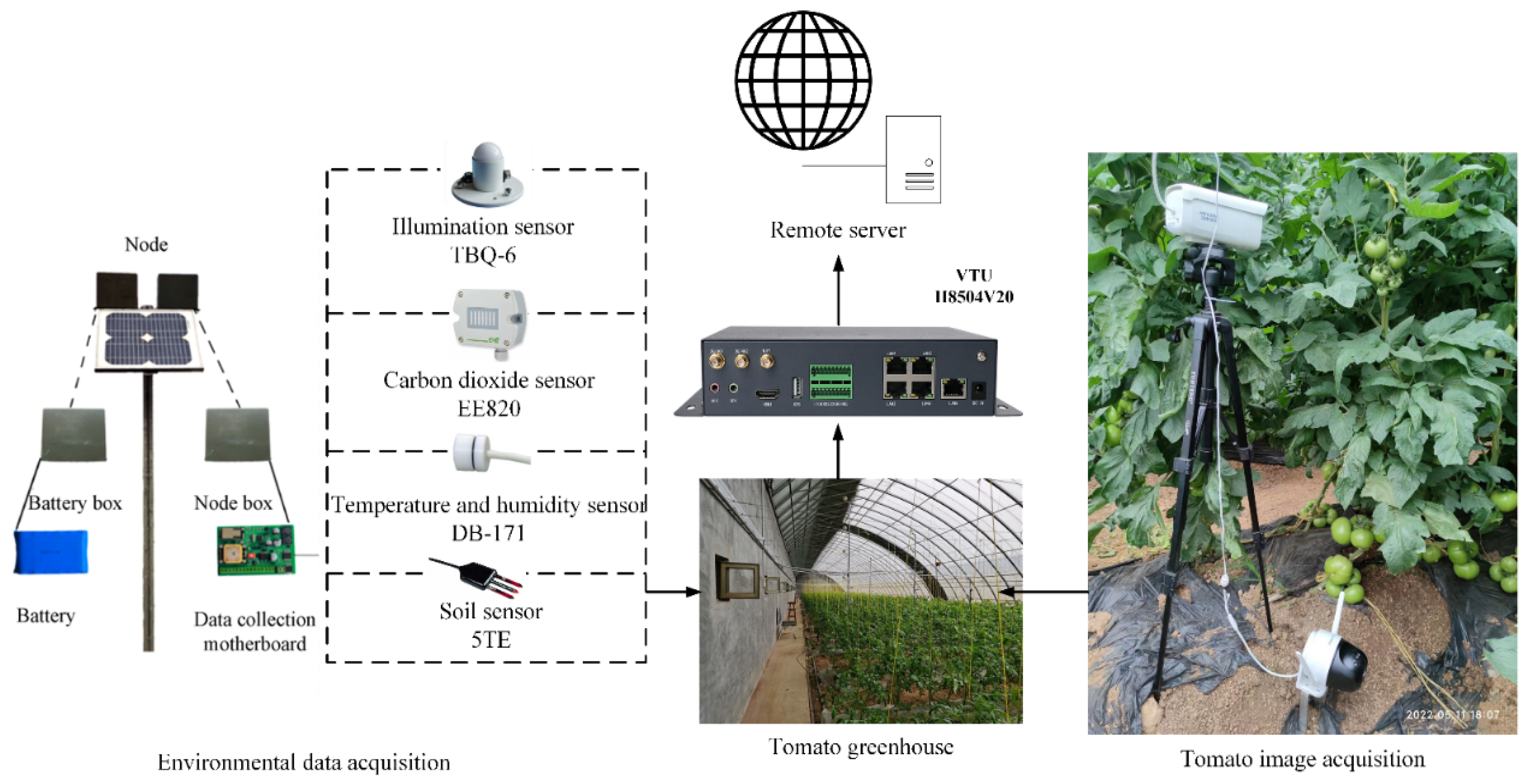
The IoT environment data acquisition system is mainly composed of the CPU, perception module, and transmission module. The core of coordinating the work of each module and ensuring the stable operation of the system is the CPU, which can realize the functions of data storage, data analysis, and data interaction. The sensing module realizes the accurate perception of air temperature, humidity, and light intensity through external sensing equipment. The transmission module uploads the collected information to the server in real time through the IoT transmission device. Parameters of the IoT sensors are shown in Table 4. A 5G network Dahuale orange TS2F camera is selected for image data acquisition, with a resolution of 4 million HD, rotating with head, including levelness and verticality, supporting full-color night vision. The camera is installed at a height consistent with the tomato fruit, maintaining a horizontal distance of about 50 cm. The captured images have a resolution of 1920 × 1080 pixels, and all camera parameters are set to the default mode. The data acquisition system architecture is shown in Figure 1.
Table 4.
Parameters of environmental sensors.
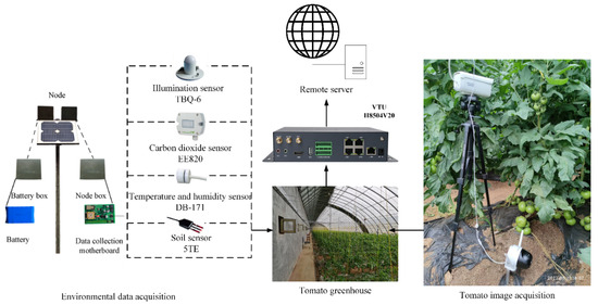
Figure 1.
The system architecture of data acquisition.
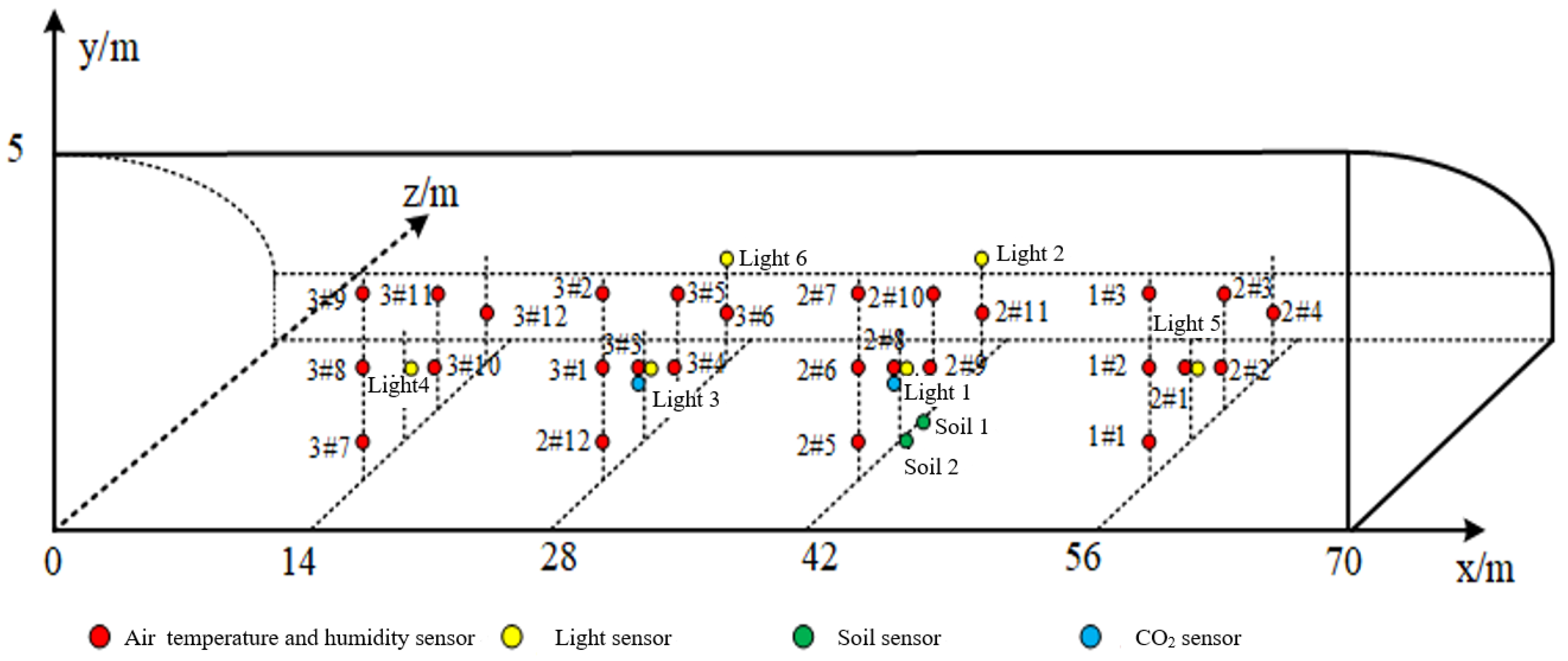
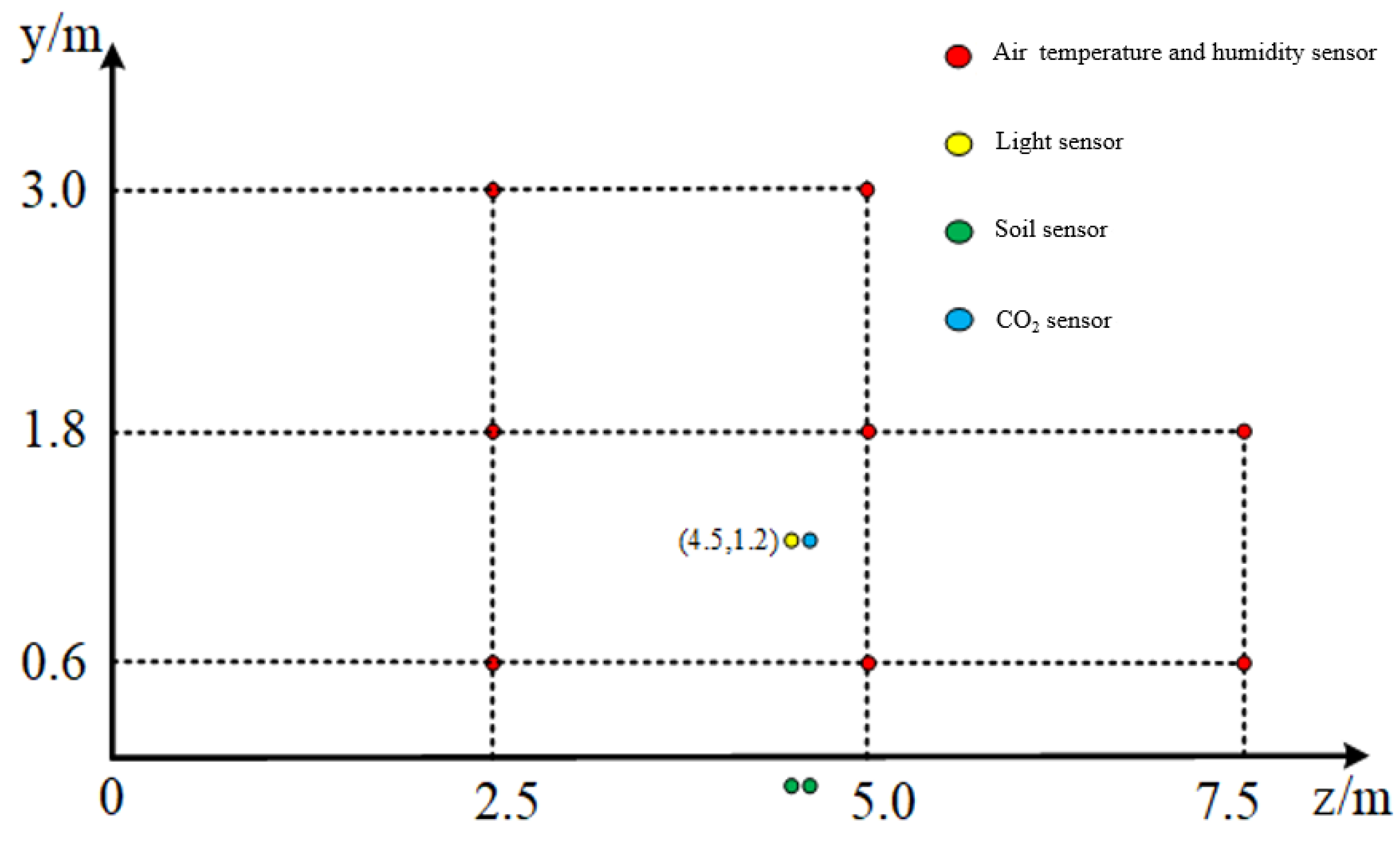
To reduce the measurement error of the sensors and ensure the effective monitoring of the greenhouse environment, multiple groups of sensors are uniformly distributed in the greenhouse. In the height direction, the sensors are arranged in the 0.6 m, 1.8 m, and 3.0 m planes. In the north–south direction, the greenhouse is divided into four parts with 2.5 m as a unit, and sensors are arranged at 2.5 m, 5 m, and 7.5 m. In the east–west direction, the greenhouse is divided into five parts in units of 14 m, and sensors are placed at 14 m, 28 m, 42 m, and 56 m. The stereo diagram and side view of the sensor deployment point are shown in Figure 2 and Figure 3, respectively.
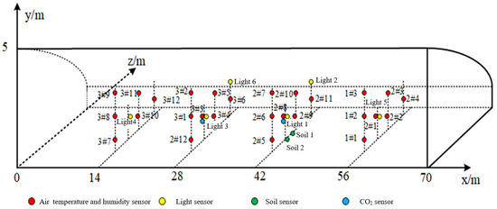
Figure 2.
The stereogram layout of the IoT sensors.
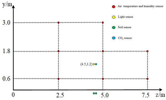
Figure 3.
Strakes layout of sensors.
2.4. Tomato Image Preprocessing and Data Set Production
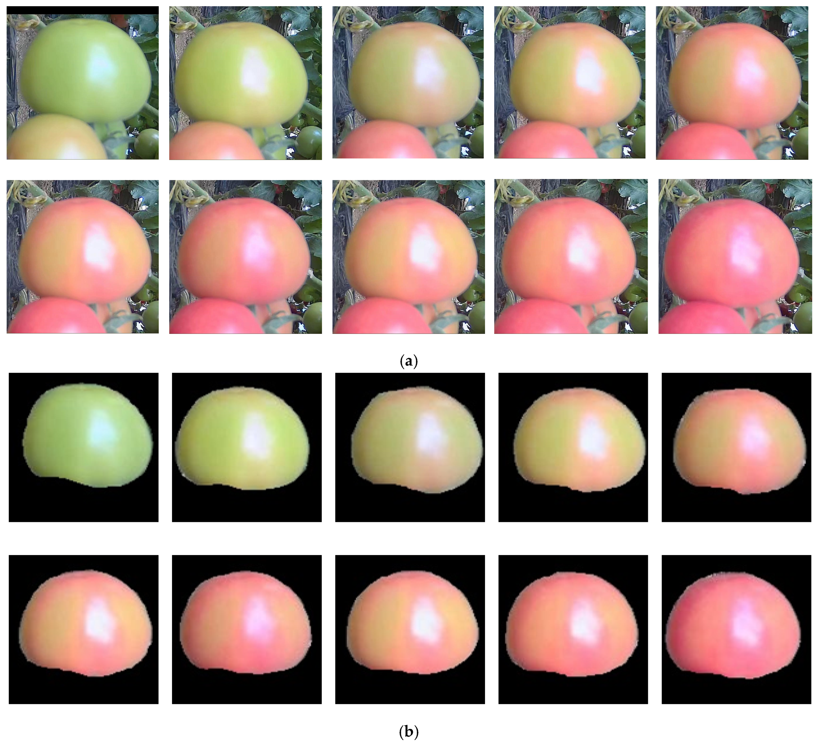
The image data were collected from the green ripening stage to the complete ripening stage, and real-time monitoring was conducted by the Dahua TS2F camera equipment (Zhejiang Dahua Technology Co., Ltd., Hangzhou, China). A total of 49 images of tomatoes were retained, and each tomato sequence contained 10 image data points, with numbers 1–5 as input sequences and numbers 6–10 as output sequences. The tomato image size was adjusted to 128 × 128 pixels. The .json files obtained by Labelme annotation were converted into mask .png files in batches to obtain the tomato mask images to reduce the interference of background noise. The tomato images before and after removing the background are shown in Figure 4. To enhance the richness of the data, the original data are rotated and enhanced by 90°, 180°, and 270°. The 1960 image data points after data enlargement were numbered in chronological order, among which 1600 were training data and 360 were validation data.
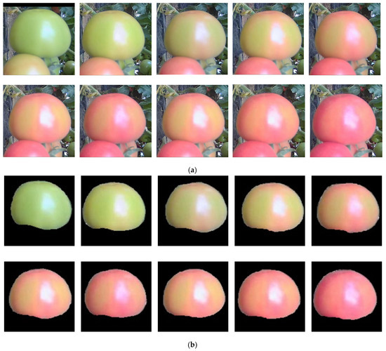
Figure 4.
Tomato images. (a) The original tomato image. (b) The tomato image with removed background information.
3. Spatial–Temporal Prediction Model
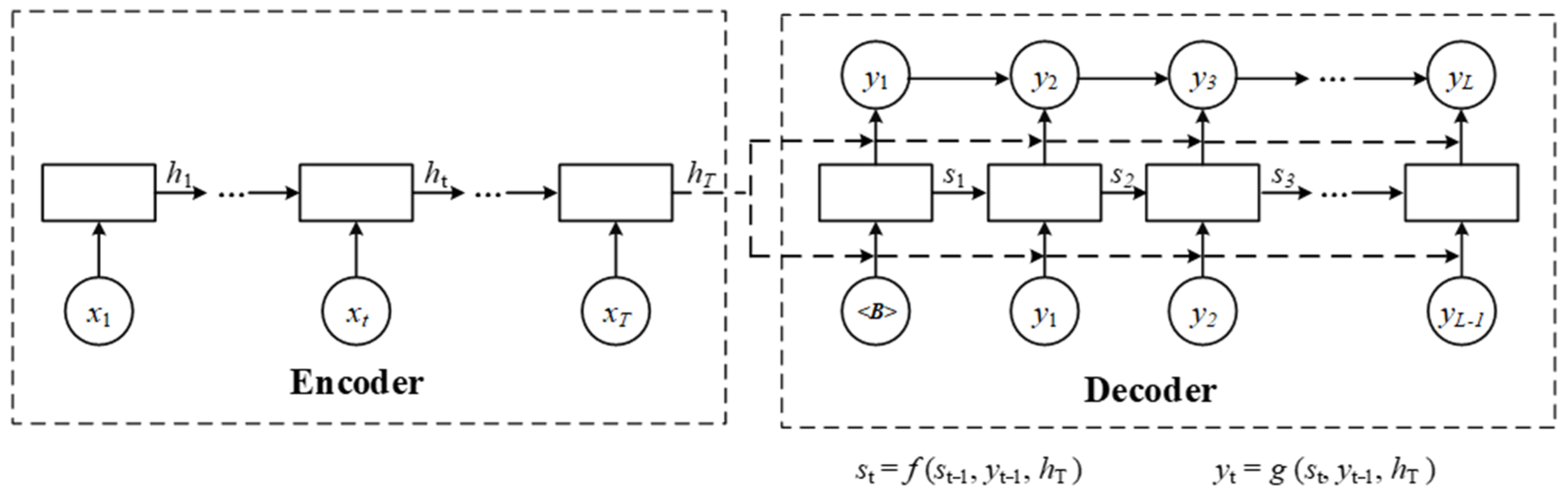
With the passage of time, tomato color will change dynamically in the space dimension. Compared with traditional data, tomato color is dependent on the time dimension and space dimension, so it is necessary to consider the influence of different positions in space. Therefore, the tomato growth data set belongs to the spatial–temporal series data [24]. To take into account both the time and space dimensions, Zaremba et al. proposed the RNN structure, which can deal with the problem of spatial–temporal series prediction. A schematic representation of a typical structure of an RNN encoder–decoder is shown in Figure 5. However, the RNN is prone to the problems of gradient disappearance and gradient explosion, so it only has short-term memory [25]. The introduction of the long short-term memory network (LSTM) solves the problem of the RNN, but the internal structure of the LSTM is complex, and the training efficiency is low. The emergence of the gated recurrent unit network (GRU) solves the above problems. In this paper, the dependent variable is set as tomato color while the independent variable is air temperature. To fully utilize spatial–temporal information, historical data of tomatoes are analyzed to predict future growth states through multi-step spatial–temporal prediction. Additionally, a two-dimensional image representation of the tomato growth data set is studied to reflect its growth state in an intuitive manner.
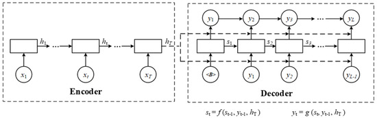
Figure 5.
The encoder–decoder structure.
The image sequence at time t is defined as , where w, h, and c denote the width, height, and channel of the image, respectively. Historical tomato images are given to predict future tomato images . The prediction of the tomato growth state is expressed by Formula (1), where denotes the maximum likelihood function.
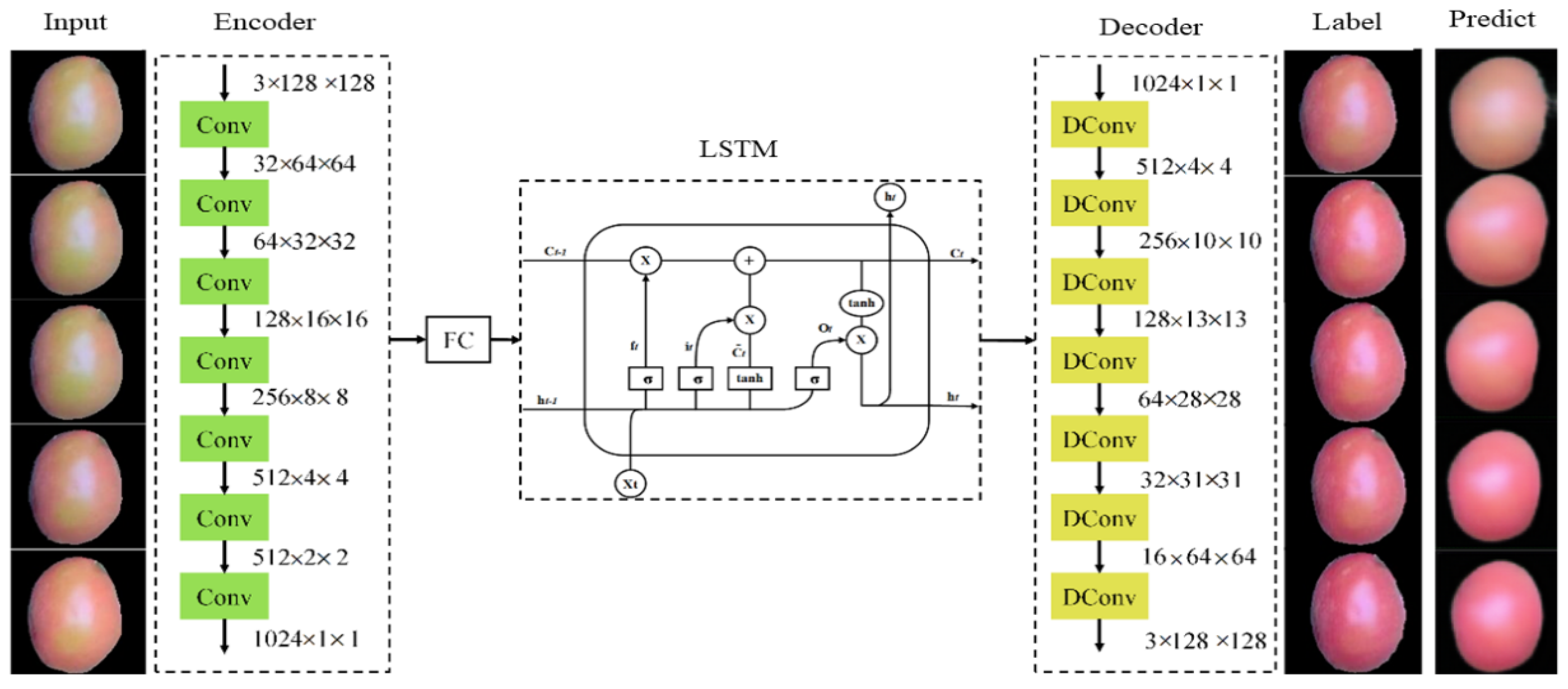
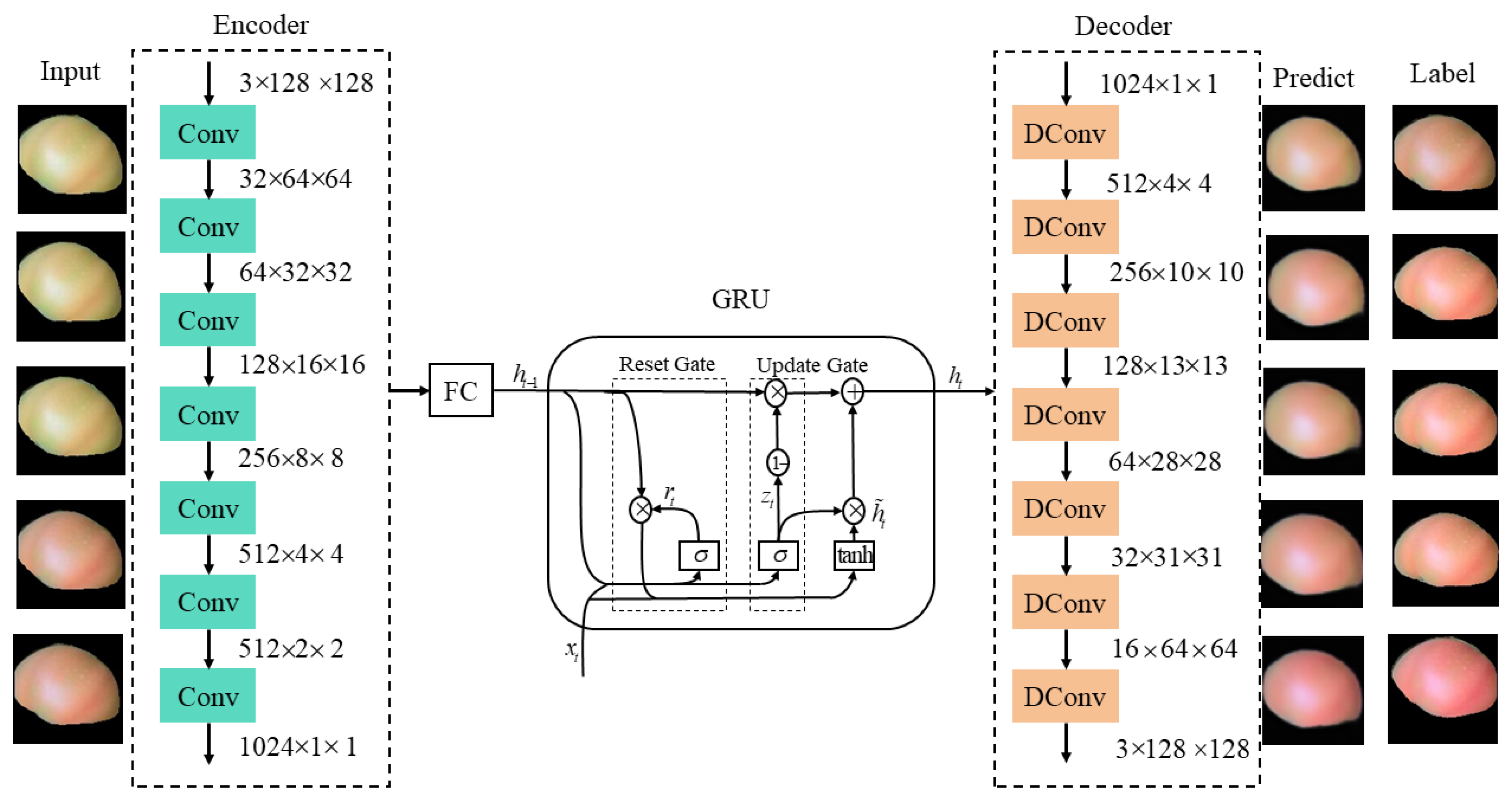
In this paper, LSTM and GRU composed of an encoder–decoder structure are used to predict the growth of tomatoes. The encoder–decoder structure can encode the growth pattern of tomatoes and effectively simulate the tomato growth phenotype. The encoder structure is to convert the original input signal into an intermediate representation, and the decoder structure is to convert the intermediate representation into the target output. Here, the encoder structure is composed of 7 convolutional layers, and the convolutional layer is used to process the input picture and convert the picture form into the intermediate representation, i.e., the time and space features of the input data sequence are extracted, and the output is used as the input of the GRU layer. The GRU layer is used to remember the tomato state and establish time dependence. Deconvolution is used in the decoder structure to convert the intermediate representation into two-dimensional image form for output.
3.1. LSTM Networks
The activation function of the LSTM network is the identity function with a derivative of 1.0, and the problem of gradient disappearance and gradient explosion in the process of long sequence training of the RNN can be solved [26,27]. The LSTM resolves the problem of long-term dependence through gate units, which includes the forgetting gate, input gate, and output gate. Compared with a traditional RNN network, the LSTM also has a neural unit state used to store historical information. However, the internal structure of the LSTM unit is complex and requires a long time for training [28]. The structure of the LSTM is shown in Figure 6, and the work flow is described by Formulas (2)–(7).
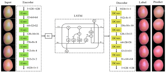
Figure 6.
LSTM model with encoder–decoder structure.
denotes the cell state at the current moment, represents the cell state at the previous moment, denotes the cell state update value, represents the forgetting gate, is the input gate, is the output gate, is the sigmoid activation function, is the hyperbolic tangent activation function, bf, bi, bo and bc represent bias entry, denotes the input, denotes the LSTM output of the current hidden layer, denotes the output of the hidden layer before LSTM, and Wf, Wi, Wo and Wc represent weight matrix.
3.2. GRU Network
Due to the complex structure, many parameters, high time cost, waste of computing resources, and other problems of the LSTM network, this paper chooses GRU, whose performance is equivalent to that of the LSTM network. The structure is shown in Figure 7. GRU is an improvement over the LSTM [29], which simplifies the internal structure of the LSTM by simplifying the three gate structures of the LSTM into two gate structures, consisting of a reset gate and an update gate. This operation reduces the parameters required for training and determines the weight of the historical data series through the control of the gate. The convergence speed of the model is fast, and the training time is shortened. Among them, the function of the update gate is to control the historical information transmitted from the previous point in time to the current point in time, and the reset gate determines the degree of historical information being forgotten [29]. The calculation of the gated cycle unit network is shown in Formulas (8)–(11):
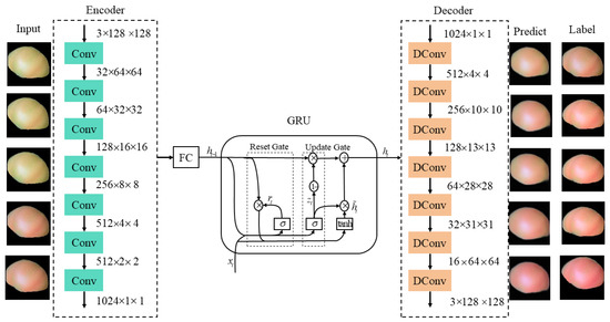
Figure 7.
GRU model with encoder–decoder structure.
denotes the input, stands for the reset gate, represents the update gate, represents the reset gate weight matrix, represents the update gate weight matrix, represents the candidate hidden state weight matrix, represents the hidden layer output, and represents the candidate hidden status.
4. Experimental Results and Analysis
4.1. Experimental Platform
The computer hardware configuration utilized in the experiment is as follows: Windows 10 operating system, an Intel(R) Core (TM) i5-8400 CPU running at 2.8~2.81 GHz, an NVIDIA GeForce RTX 3060 Ti GPU (Colorful Group, Shenzhen, China), and a Python 3.7 software framework. The computer hardware configuration used in the experiment is as follows: the operating system is Windows 10, wherein the CPU is an Intel(R) Core (TM) i5-8400 CPU @ 2.8~2.81 GHz, the GPU is an NVIDIA GeForce RTX 3060 Ti, and the software framework is Python 3.7.
4.2. Model Training
The L1 loss function is used, Adam is employed as the optimizer, and the ReduceLROnPlateau learning rate decay strategy is applied, with the initial learning rate set as 10-4. The batch size is 8, and the maximum number of iterations is set to 10,000. To prevent overfitting, dropout regularization is implemented, and an early stopping strategy is applied on the validation set. Different hidden layer numbers, hidden unit numbers, and different RNN structures are selected to discuss the effect of the model on predicting tomato growth, selecting LSTM and GRU as the RNN structures respectively.
4.3. Results and Analysis
The Structural Similarity Index Measure (SSIM) has been chosen as the evaluation metric to assess the proposed model’s similarity between the forecasted data and the actual tomato image. SSIM is employed to more accurately measure and predict the overall visual image quality of tomatoes. The closer the SSIM is to 1, the more similar the two images are in contrast, brightness, and structure [30]. Table 5 shows the indexes of the LSTM and GRU models of encoder and decoder structure. The SSIM value of the GRU model is 0.008 higher than that of the LSTM model of the encoder–decoder structure. The size of the model is reduced by 30 MB and the model is easier to train.
Table 5.
Comparison of LSTM and GRU model with encoder-decoder architecture.
4.3.1. Influence of Different Network Structures on Prediction Performance
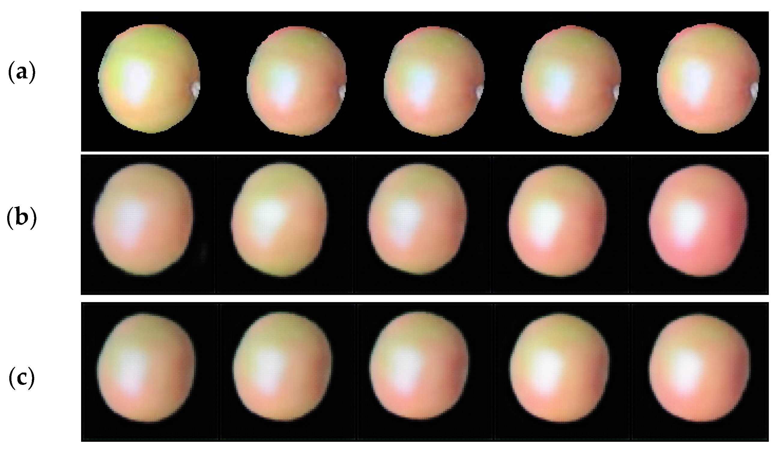
To select suitable prediction models for tomato growth, the LSTM and GRU models of encoder–decoder structure are analyzed. Compared with the LSTM network structure, GRU uses an update gate to select and forget information at the same time, which improves its efficiency. Experimental results confirmed that the GRU network with encoder–decoder structure is more suitable for tomato fruit growth prediction during the color turning stage. Tomato growth prediction results are shown in Figure 8. In terms of tomato shape prediction, the LSTM model with encoder–decoder structure and the GRU model have similar prediction effects, but the GRU model is closer to the real tomato growth situation in terms of tomato color prediction.
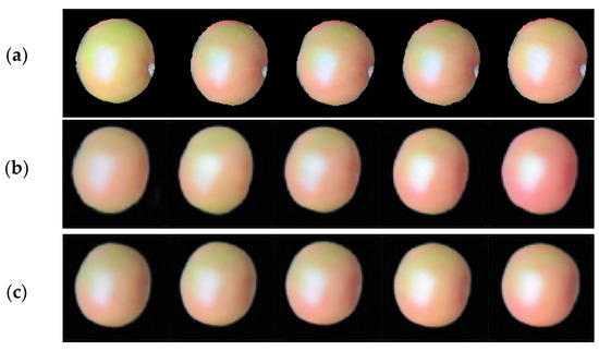
Figure 8.
Tomato growth prediction results of LSTM and GRU models with encoder–decoder structure. (a) Real tomato images, (b) LSTM tomato growth prediction results, and (c) GRU tomato growth prediction results.
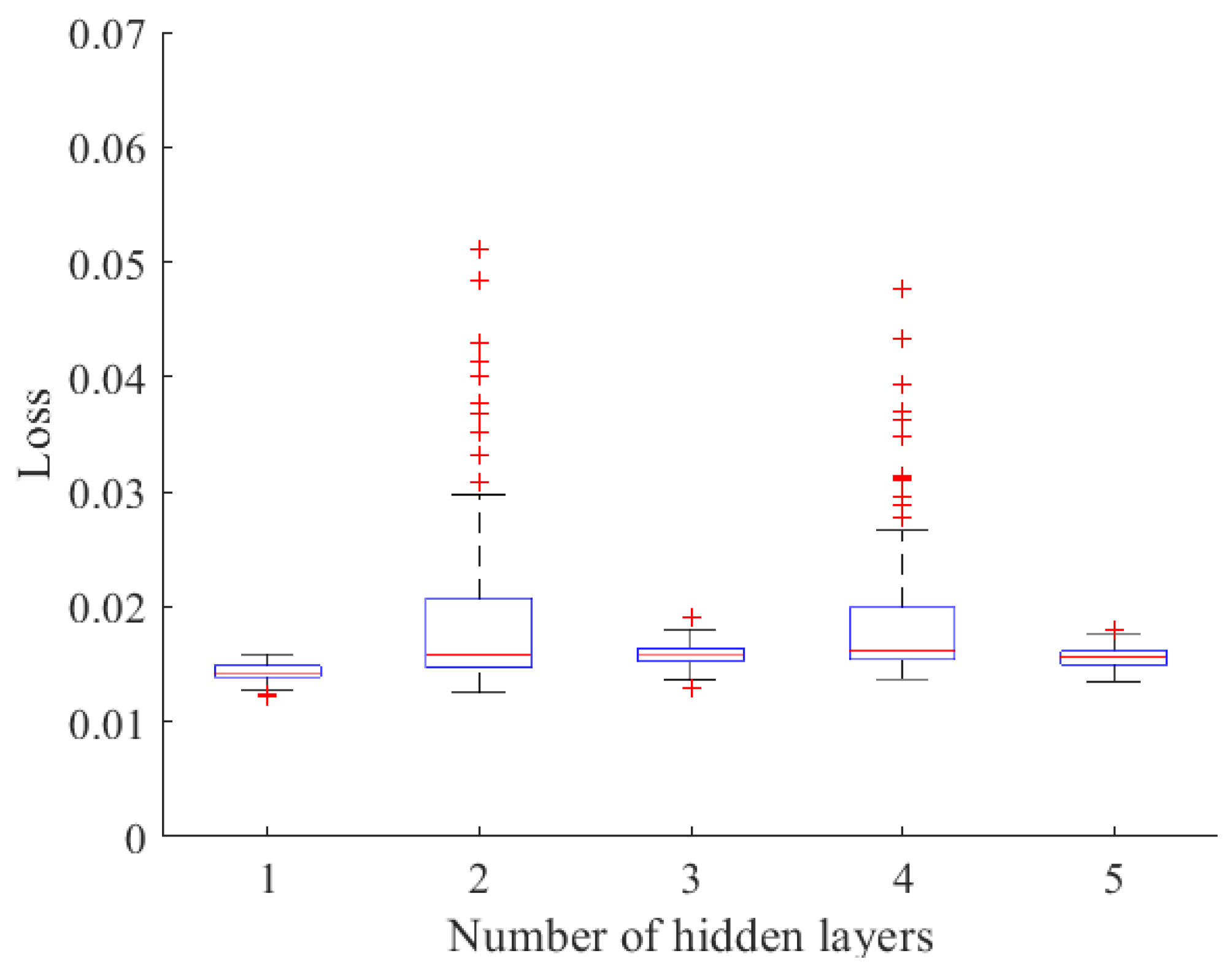
The number of hidden layers has a great impact on model performance. Therefore, the hidden layers of the network are set as 1–6 in this study. As shown in Table 6, the models with odd numbers of hidden layers are better than the models with even number of hidden layers in predicting tomato growth color. As the number of network layers increases, the model training will be more difficult, the overfitting will be more serious, and the effect of shape and color prediction will become worse. In this study, the model with the least number of layers but the performance second only to the optimal performance is chosen as hidden layer number 1. Figure 9 shows the change curve of loss value in the last 100 rounds of training. When the number of hidden layers is 1, there are two specific points, both of which are low specific points, indicating that the loss value is lower than other loss values, the loss value is small, and the fluctuation range is small.
Table 6.
SSIM index of different hidden layers in GRU model of encoder–decoder structure.
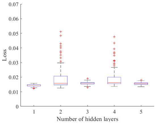
Figure 9.
Loss values for the last 100 rounds.
4.3.2. Influence of Different Number of Hidden Layer Units on the Prediction Performance
Parameter adjustment directly affects the performance of the model. In this study, the number of hidden layer units of the model is set as 32, 64, 128, 256, 512, and 1024. The loss function curve of the model is shown in Figure 10. The number of hidden layer elements selected in this paper is 512. It can be seen from the loss curve that the model is easier to train, the loss value is the lowest after 100 rounds, and the model has the best convergence effect. Table 7 shows the SSIM values of the model training real image and the predicted image under different elements of the hidden layer. When the number of elements of the hidden layer is set to 512, the SSIM value of 0.77 is the highest, indicating the best performance of the model. The predicted results of the tomato growth trend have a high consistency with the actual growth trend of tomatoes. When the number of hidden layer elements is small, the ability of the model to extract features is poor, and there is a large gap between the tomato growth prediction effect and the actual tomato growth. If the number of hidden layer elements is too large, the calculation cost and size of the model will be increased.
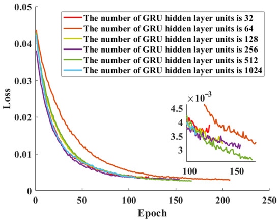
Figure 10.
Comparison of loss function curves of GRU models with different numbers of hidden layer units in the encoder–decoder structure.
Table 7.
SSIM index of number of units in different hidden layers for GRU model of encoder–decoder structure.
4.3.3. The Influence of Environmental Conditions on the Prediction Performance
The tomato fruit mature in stages from bottom to top, so the greenhouse environment of fruits with different ripening times is slightly different. One spike, three spikes, and five spikes are selected for the color change prediction research. The color change date and corresponding environmental data of the selected fruits are shown in Table 8.
Table 8.
Environmental parameters of different fruit stages.
As can be seen from Table 8, air temperature, light intensity, and soil temperature are the major environmental differences between tomatoes with different ripening dates, while other environmental factors have no obvious differences and change rules. Temperature has an important influence on the growth and development of tomatoes. Low temperature is likely to lead to slow development and delayed fruit ripening, which has a great influence on its early maturity and high yield, and also affects the synthesis of lycopene. High temperature is likely to lead to premature plant aging, lower fruit setting rate and smaller fruit size [31]. The prediction results are shown in Figure 11. Input t − 4, t − 3, t − 2, t − 1, and t time to predict the growth of tomato at t + 1, t + 2, t + 3, t + 4, and t + 5 time. With the increase in temperature and light intensity, the color change time of tomato is shortened, and the time from the green ripening stage to the red ripening stage is about 10.5 days, 8.3 days, and 7.1 days, which confirms that the greenhouse environment of five spikes is more suitable for the color change of tomatoes at the maturity stage. When the greenhouse environment maintains a temperature at 24.93 °C, light intensity at 11.26 Klux, and soil temperature at 24.06 °C, it is conducive to lycopene production, which aligns with the findings of Shamshiri et al. [32].
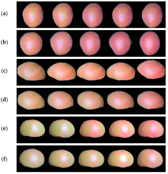
Figure 11.
Prediction results of tomato colors at different stages (environment): (a) real tomato images at five panicles, (b) prediction results for tomatoes at five panicles; (c) real tomato images at three panicles; (d) prediction results for tomatoes at three panicles, (e) real tomato images at the first panicle, and (f) prediction results for tomatoes at the first panicle.
5. Conclusions
Most phenotypic studies of plants focus on leaves or entire plants [33], with Arabidopsis thaliana being a typical representative [23]. Studying the growth trends of plants to understand breeding cycles is crucial for agricultural development [34]. The color and shape of a tomato determines the nutritional and economic value of the tomato in the market. Phenotypic traits provide an intuitive method to assess tomato growth status, enabling clear observation of external morphological characteristics such as color and shape. Research on tomato phenotype prediction holds significant importance for guiding tomato growth.
The goal of this paper is to use the historical color features of tomatoes to predict the future growth trends in color and shape, constructing a time-dependent relationship. Due to the inherent randomness in crop growth and development, prediction accuracy based on crop growth models is typically not high. Consequently, scholars have introduced machine vision technology and proposed spatiotemporal prediction methods based on image monitoring.
Sakurai et al. [33] employed convolutional networks to extract key features from leaf images and combined LSTM with encoder–decoder models to forecast leaf growth. This approach utilizes the ConvLSTM model to predict future growth images based on historical sequences, extracting temporal growth correlations via LSTM and spatial correlations via convolution to achieve deep feature fusion across both temporal and spatial dimensions in plant growth prediction. This method first demonstrated the feasibility of using ConvLSTM for spatiotemporal prediction in crop growth, achieving a modest prediction accuracy of 72.8%. Aigner et al. [35] utilized generative adversarial networks to train FutureGAN networks, learning the historical growth trends of crops and applying them to predict the growth of plant leaves and roots. However, this model relies on crop masks for predictions, overlooking crop texture and color information. To address this issue, Wang et al. [36] proposed the spatiotemporal long short-term memory model, ST-LSTM, to forecast the growth and development of Arabidopsis based on a background-noise-filtered RCB continuous growth and development map. The similarity of the predicted structures reached 0.87. However, as the prediction horizon increases, results become increasingly blurry, and the method does not assess the consistency of actual leaf position and shape. Yang et al. [37] proposed a spatiotemporal prediction algorithm for mushroom growth status based on historical time series growth images, facilitating early bud thinning to prevent the formation of dense mushroom clusters. The algorithm employs a sequence-to-sequence structure comprising an encoder and a predictor, achieving a multiscale structure similarity of 0.927.
However, there is a lack of relevant research on predicting tomato color changes. Building on existing research, this paper proposes a GRU network with an encoder–decoder structure to predict tomato color changes in conjunction with tomato growth and environmental data. The tomato growth process is visualized, and predictions for greenhouse tomato growth are analyzed under different configurations of hidden layers and units. Experimental results demonstrate that the proposed model exhibits high consistency with actual tomato growth states, achieving an SSIM of 0.746. The model performs well with a single hidden layer and 512 hidden layer units. It was found that an average temperature of 24.93 °C, average soil temperature of 24.06 °C, and average light intensity of 11.26 Klux are optimal for tomato growth. Conversely, environmental factors such as average air humidity, carbon dioxide concentration, soil moisture, and soil concentration have minimal influence on tomato growth predictions, consistent with findings by Shamshiri et al. [32].
This study provides a theoretical foundation for investigating suitable greenhouse environmental conditions for tomato cultivation and accurate timing for harvesting. Furthermore, it offers theoretical and technical guidance for the precise regulation and automated management of tomato growth in solar greenhouses.
Although our model performed well in experimental testing, there are still some limitations. One of the limitations is the potential variability in environmental conditions, which may not have been fully captured in our current dataset. Variations in factors such as pesticides and fertilizers could have an impact on tomato growth and ripening stages [38,39], and these aspects were not comprehensively addressed in our model. Moreover, our model is limited to solar greenhouses; its generalizability to other cultivation settings and tomato varieties has not been extensively evaluated. Different greenhouse designs and genetic variations in tomatoes may lead to unique growth patterns that were not fully accounted for in our research.
Based on the above analysis, in future work, we will attempt to focus on incorporating a wider range of environmental parameters into the predictive model, allowing for a more holistic understanding of the factors influencing tomato growth and color change. In addition, we will try to enhance the generalizability of the model, to adapt the predictive model to different greenhouse environments and tomato varieties. This may involve collecting diverse datasets from various cultivation settings and leveraging techniques to transfer knowledge gained from one context to another. Furthermore, future research could focus on validating the practical implementation of the model in real-world agricultural settings. Field trials and feedback from growers could provide valuable insights into the performance of the model under diverse conditions and guide refinements for practical applicability.
Author Contributions
Data curation, H.Y. and T.L.; investigation, S.L.; methodology, Y.Z.; software, S.L.; supervision, T.L. and L.Z.; validation, L.Z. and S.C.; visualization, S.C.; writing—original draft, S.L., H.Y. and Y.Z.; writing—review and editing, H.Y. and L.Z. All authors have read and agreed to the published version of the manuscript.
Funding
This research was supported by the Major Science and Technology Innovation Project of Shandong Province (2022CXGC020708) and the Science and Technology smes innovation ability improvement project of Shandong Province (2022TSGC2047).
Institutional Review Board Statement
Not applicable.
Data Availability Statement
All data are presented in this article in the form of figures and tables.
Acknowledgments
The authors would like to thank the editors and all the reviewers who participated in the review.
Conflicts of Interest
The authors declare no conflicts of interest.
References
- López-Correa, J.M.; Moreno, H.; Ribeiro, A.; Andújar, D. Intelligent Weed Management Based on Object Detection Neural Networks in Tomato Crops. Agronomy 2022, 12, 2953. [Google Scholar] [CrossRef]
- Wang, X.; Liu, J. Tomato anomalies detection in greenhouse scenarios based on YOLO-Dense. Front. Plant. Sci. 2021, 12, 634103. [Google Scholar] [CrossRef] [PubMed]
- Nagase, K.; Shiraki, T.; Iwasaki, H. Plant factory solution with instrumentation and control technology. Fuji Electr. Rev. 2016, 62, 160–164. [Google Scholar]
- Chen, L.; Pan, Y.; Li, H.; Liu, Z.; Jia, X.; Li, W.; Jia, H.; Li, X. Constant temperature during postharvest storage delays fruit ripening and enhances the antioxidant capacity of mature green tomato. J. Food Process. Pres. 2020, 44, e14831. [Google Scholar] [CrossRef]
- Li, N.; Wu, X.; Zhuang, W.; Xia, L.; Chen, Y.; Wu, C.; Rao, Z.; Du, L.; Zhao, R.; Yi, M. Tomato and lycopene and multiple health outcomes: Umbrella review. Food Chem. 2021, 343, 128396. [Google Scholar] [CrossRef]
- Kaur, K.; Gupta, O. A machine learning approach to determine maturity stages of tomatoes. Orient. J. Comput. Sci. Technol. 2017, 10, 683–690. [Google Scholar] [CrossRef]
- Su, F.; Zhao, Y.; Wang, G.; Liu, P.; Yan, Y.; Zu, L. Tomato Maturity Classification Based on SE-YOLOv3-MobileNetV1 Network under Nature Greenhouse Environment. Agronomy 2022, 12, 1638. [Google Scholar] [CrossRef]
- Jerca, I.O.; Cîmpeanu, S.M.; Teodorescu, R.I.; Drăghici, E.M.; Nițu, O.A.; Sannan, S.; Arshad, A. A Comprehensive Assessment of the Morphological Development of Inflorescence, Yield Potential, and Growth Attributes of Summer-Grown, Greenhouse Cherry Tomatoes. Agronomy 2024, 14, 556. [Google Scholar] [CrossRef]
- Ghavami, M. Development of Internet of Things Based Smart Multi-Sensors System for Early Prediction of Plant Growth. Master’s Thesis, University of Manitoba, Winnipeg, MB, Canada, 2022. Available online: http://hdl.handle.net/1993/36507 (accessed on 27 May 2022).
- Liu, Y.; Tan, R.; Guo, W.; Zheng, W.; Zhang, X.; Xu, F.; Chen, X. Sensitivity analysis of secondary metabolites in tomato fruits to low light treatment at the different growth stages. Trans. Chin. Soc. Agric. Eng. 2023, 39, 211–220. [Google Scholar] [CrossRef]
- Barrett, D.M.; Beaulieu, J.C.; Shewfelt, R. Color, flavor, texture, and nutritional quality of fresh-cut fruits and vegetables: Desirable levels, instrumental and sensory measurement, and the effects of processing. Crit. Rev. Food Sci. 2010, 50, 369–389. [Google Scholar] [CrossRef]
- Sugino, N.; Watanabe, T.; Kitazawa, H. Effect of transportation temperature on tomato fruit quality: Chilling injury and relationship between mass loss and a* values. J. Food Meas. Charact. 2022, 16, 2884–2889. [Google Scholar] [CrossRef]
- Kuijpers, W.J.; van de Molengraft, M.; van Mourik, S.; van’t Ooster, A.; Hemming, S.; van Henten, E.J. Model selection with a common structure: Tomato crop growth models. Biosyst. Eng. 2019, 187, 247–257. [Google Scholar] [CrossRef]
- Samal, S.; Acharya, B.; Barik, P.K. Internet of Things (IoT) in agriculture toward urban greening. In AI, Edge and IoT-Based Smart Agriculture; Elsevier: Amsterdam, The Netherlands, 2022; pp. 171–182. [Google Scholar] [CrossRef]
- Ayaz, M.; Ammad-Uddin, M.; Sharif, Z.; Mansour, A.; Aggoune, E.H.M. Internet-of-Things (IoT)-based smart ag-riculture: Toward making the fields talk. IEEE Access 2019, 7, 129551–129583. [Google Scholar] [CrossRef]
- Ting, L.; Yuhan, J.; Man, Z.; Sha, S.; Minzan, L. Universality of an improved photosynthesis prediction model based on PSO-SVM at all growth stages of tomato. Int. J. Agric. Biol. Eng. 2017, 10, 63–73. [Google Scholar] [CrossRef]
- Harun, A.N.; Mohamed, N.; Ahmad, R.; Ani, N.N. Improved Internet of Things (IoT) monitoring system for growth optimization of Brassica chinensis. Comput. Electron. Agric. 2019, 164, 104836. [Google Scholar] [CrossRef]
- Liao, M.S.; Chen, S.F.; Chou, C.Y.; Chen, H.Y.; Yeh, S.H.; Chang, Y.C.; Jiang, J.A. On precisely relating the growth of Phalaenopsis leaves to greenhouse environmental factors by using an IoT-based monitoring system. Comput. Electron. Agric. 2017, 136, 125–139. [Google Scholar] [CrossRef]
- Kocian, A.; Massa, D.; Cannazzaro, S.; Incrocci, L.; Di Lonardo, S.; Milazzo, P.; Chessa, S. Dynamic Bayesian network for crop growth prediction in greenhouses. Comput. Electron. Agric. 2020, 169, 105167. [Google Scholar] [CrossRef]
- Cisternas, I.; Velásquez, I.; Caro, A.; Rodríguez, A. Systematic literature review of implementations of precision agriculture. Comput. Electron. Agric. 2020, 176, 105626. [Google Scholar] [CrossRef]
- Del Borghi, A.; Tacchino, V.; Moreschi, L.; Matarazzo, A.; Gallo, M.; Vazquez, D.A. Environmental assessment of vegetable crops towards the water-energy-food nexus: A combination of precision agriculture and life cycle assessment. Ecol. Indic. 2022, 140, 109015. [Google Scholar] [CrossRef]
- Jiang, Z.; Liu, C.; Hendricks, N.P.; Ganapathysubramanian, B.; Hayes, D.J.; Sarkar, S. Predicting county level corn yields using deep long short term memory models. arXiv 2018, arXiv:1805.12044. [Google Scholar] [CrossRef]
- Yasrab, R.; Zhang, J.; Smyth, P.; Pound, M.P. Predicting plant growth from time-series data using deep learning. Remote Sens. 2021, 13, 331. [Google Scholar] [CrossRef]
- Zhu, Q.; Chen, J.; Zhu, L.; Duan, X.; Liu, Y. Wind speed prediction with spatio–temporal correlation: A deep learning approach. Energies 2018, 11, 705. [Google Scholar] [CrossRef]
- Zaremba, W.; Sutskever, I.; Vinyals, O. Recurrent neural network regularization. arXiv 2015, arXiv:1409.2329. [Google Scholar] [CrossRef]
- Bengio, Y.; Simard, P.; Frasconi, P. Learning long-term dependencies with gradient descent is difficult. IEEE. T. Neural. Networ. 1994, 5, 157–166. [Google Scholar] [CrossRef]
- Graves, A. Long short-term memory. In Supervised Sequence Labelling with Recurrent Neural Net-Works; Springer: Berlin, Germany, 2012; Volume 9, pp. 37–45. [Google Scholar]
- Wang, Z.; Li, Y.; Li, Z.; Zhao, C.; Gao, F.; Wang, P. Reduced-order DC terminal dynamic model for multi-port AC-DC power electronic transformer. Energies 2019, 12, 2130. [Google Scholar] [CrossRef]
- Wang, Y.; Liao, W.; Chang, Y. Gated recurrent unit network-based short-term photovoltaic forecasting. Energies 2018, 11, 2163. [Google Scholar] [CrossRef]
- Wang, Z. Applications of objective image quality assessment methods [applications corner]. IEEE Signal Proc. Mag. 2011, 28, 137–142. [Google Scholar] [CrossRef]
- Lee, K.; Rajametov, S.N.; Jeong, H.-B.; Cho, M.-C.; Lee, O.-J.; Kim, S.-G.; Yang, E.-Y.; Chae, W.-B. Comprehensive Understanding of Selecting Traits for Heat Tolerance during Vegetative and Reproductive Growth Stages in Tomato. Agronomy 2022, 12, 834. [Google Scholar] [CrossRef]
- Shamshiri, R.R.; Jones, J.W.; Thorp, K.R.; Ahmad, D.; Man, H.C.; Taheri, S. Review of optimum temperature, humidity, and vapour pressure deficit for microclimate evaluation and control in greenhouse cultivation of tomato: A review. Int. Agrophys. 2018, 32, 287–302. [Google Scholar] [CrossRef]
- Sakurai, S.; Uchiyama, H.; Shimada, A.; Taniguchi, R. Plant Growth Prediction using Convolutional LSTM. In Proceedings of the 14th International Joint Conference on Computer Vision, Imaging and Computer Graphics Theory and Applications (VISIGRAPP 2019), Prague, Czech Republic, 25–27 February 2019; pp. 105–113. [Google Scholar] [CrossRef]
- Rizkiana, A.; Nugroho, A.; Salma, N.; Afif, S.; Masithoh, R.; Sutiarso, L.; Okayasu, T. Plant growth prediction model for lettuce (Lactuca sativa.) in plant factories using artificial neural network. IOP Conf. Ser. Earth Environ. Sci. 2021, 733, 012027. [Google Scholar] [CrossRef]
- Aigner, S.; Krner, M. FutureGAN: Anticipating the Future Frames of Video Sequences using Spatio-Temporal 3d Convolutions in Progressively Growing GANs. arXiv 2018, arXiv:1810.01325. [Google Scholar] [CrossRef]
- Wang, C.; Pan, W.; Li, X.; Liu, P. Plant Growth and Development Prediction Model Based on ST-LSTM. Trans. Chin. Soc. Agric. Mach. 2022, 53, 250–258. [Google Scholar]
- Yang, S.; Huang, J.; Yuan, J. Spatiotemporal Prediction Algorithm for Mushroom Growth Status Based on Improved LSTM. Trans. Chin. Soc. Agric. Mach. 2024, 55, 221–230. [Google Scholar]
- Wang, C.; Wu, G.; Wang, H.; Wang, J.; Yuan, M.; Guo, X.; Liu, C.; Xing, S.; Sun, Y.; Talpur, M.M.A. Optimizing Tomato Cultivation: Impact of Ammonium–Nitrate Ratios on Growth, Nutrient Uptake, and Fertilizer Utilization. Sustainability 2024, 16, 5373. [Google Scholar] [CrossRef]
- Tommonaro, G.; Abbamondi, G.R.; Nicolaus, B.; Poli, A.; D’Angelo, C.; Iodice, C.; De Prisco, R. Productivity and Nutritional Trait Improvements of Different Tomatoes Cultivated with Effective Microorganisms Technology. Agriculture 2021, 11, 112. [Google Scholar] [CrossRef]


Disclaimer/Publisher’s Note: The statements, opinions and data contained in all publications are solely those of the individual author(s) and contributor(s) and not of MDPI and/or the editor(s). MDPI and/or the editor(s) disclaim responsibility for any injury to people or property resulting from any ideas, methods, instructions or products referred to in the content. |
© 2024 by the authors. Licensee MDPI, Basel, Switzerland. This article is an open access article distributed under the terms and conditions of the Creative Commons Attribution (CC BY) license (https://creativecommons.org/licenses/by/4.0/).