Farm Plot Boundary Estimation and Testing Based on the Digital Filtering and Integral Clustering of Seeding Trajectories

Abstract

Farmland boundary data, an important basic data for the operation of agricultural automation equipment, has been widely studied by scholars from all over the world. However, the common methods of farmland boundary acquisition through sensors such as LiDAR and vision cameras combined with complex algorithms suffer from problems such as serious data drift, difficulty in eliminating noise, and inaccurate plot boundary data. In order to solve this problem, this study proposes a method for estimating the orientation dimensions of farmland based on the seeding trajectory. The method firstly calculates the curvature of the discrete data of the seeding trajectory; secondly, we innovatively use a low-pass filter and integral clustering to filter the curvature values and distinguish between straight lines and curves; and finally, the straight-line portion located at the edge of the seeding trajectory is fitted with a univariate linear fit to calculate the estimation of the farmland size orientation. As verified by the field experiments, the minimum linear error of the vertices is only 0.12m, the average error is 0.315m, and the overlapping rate of the plot estimation is 98.36% compared with the real boundary of the plot. Compared with LiDAR mapping, the average linear error of the vertices’ position is reduced by 50.2%, and the plot estimation overlap rate is increased by 2.21%. The experimental results show that this method has the advantage of high accuracy, fast calculation speed, and small calculation volume, which provides a simple and accurate method for constructing farmland maps, provides the digital data support for the operation of agricultural automation equipment, and has significance for farm digital mapping.

1. Introduction

As the number of agricultural laborers is decreasing year by year, and the labor costs are increasing dramatically, the demand for agricultural automation is increasing steeply, and the accurate estimation of plot boundaries, as the key data necessary for agricultural automation, has become a technological need that needs to be implemented urgently [1,2,3,4]. For example, path planning for fertilizer tractors [5,6,7], operational transport planning for field robots [8,9], the estimation of crop moisture content in farmland [10,11], and the estimation of yield per unit area of farmland [12], all rely on accurate information about the boundaries of the farmland plots [13]. Therefore, the detection of the orientation and dimensions of farmland plot boundaries are the focus of researchers all over the world [14,15,16,17,18]. Due to the diversity and uncertainty of the environmental characteristics of crop cultivation, the vegetation growth pattern is different and unevenly distributed, the soil stack pattern is randomly distributed, and different soil types and colors also show obvious heterogeneity, which leads to the differences between cultivated and non-cultivated plots not being prominent enough; all these randomly distributed environmental characteristics bring certain challenges to the acquisition of farmland boundary detection.

Currently, manual GPS pointing, visual sensor perception, and LiDAR detection are often used to identify and orient the boundaries of agricultural farmland plots. The use of manual GPS pointing poses a great test of the physical strength of agricultural laborers, while changes in the light intensity and the complex terrain surface texture pose a greater challenge to the visual sensors. LiDAR is used in the detection of point cloud distortion, and the noise generated by the surrounding environment may lead to a certain degree of bias in the detection results. To address the above problems, in this study, an innovative plot boundary estimation method based on seeding paths is proposed, which involves morphological curvature computation, low-pass filtering, and linear fitting computation of the seeding trajectory, and innovatively employs non-perceptual data for the acquisition of the boundary size orientation.

Matthias from the University of Kiel [19] in Germany, used a combination of deep learning and image erosion to extract the boundary contours from photos of vacant planted farmland, to obtain farmland boundary contours. Gumma uses a deep learning algorithm and combines it with semantic segmentation to recognize the boundaries of farmland in satellite photos [20]. Borowiec uses solid-state LiDAR [21], which acquires data from the ground, and obtains the boundaries of the farmland by performing pixel density calculations with the Hough transform on the point cloud distribution.

Yan Zhang of Shanghai Jiaotong University [22] manually uses GPS to acquire the farmland boundaries and provide the farmland boundary information for the rice field autopilot control algorithms. Daoqing Cai preprocesses the image information collected by the visual camera using the simple linear iterative cluster (SLIC) algorithm for super-pixel segmentation of paddy field images, which serves as the input for the training of the support vector machine (SVM) model [23], and then segments the images and uses the Hough transform to extract the ridge boundary of the paddy field. Zhai et al. used a deep learning algorithm to analyze the farm machine path points, to distinguish the working area of the farm machine, and thus to estimate the working area of the farmland [24].

The above methods provide a good way to measure the boundaries of the operational farmland, however, obtaining plot boundaries using manual GPS requires staff to hold a positioning device and walk across the entire farmland, which is highly labor-intensive and less efficient. Cameras, satellite remote sensing, and other methods to identify and detect the boundaries of farmland through images, incur high data acquisition costs, and the image sensor is easily affected by light, thus reducing the accuracy of the data analysis [25]. LiDAR can obtain more accurate point cloud data, but the data volume is massive with a high requirement for computer resources, and when encountering weeds, soil stacks, and obstacles, the sensor produces a large noise, thus affecting perception [26,27]. Considering the current problem that it is difficult to obtain the boundaries of farmland, this paper proposes a fast and accurate estimation of the plot boundary based on the seeding trajectory data. The method innovatively integrates multiple algorithms of the path morphology curvature calculation, curvature digital low-pass filtering and integral clustering, threshold classification, and linear fitting, and can complete the estimation of the size and orientation of the farmland boundary without the use of additional sensors, using only the data from the seeding trajectories of the agricultural machines. This method uses a small amount of data, has good noise resistance, a fast calculation speed without the use of complex high-precision sensors, and the calculated results provide reliable digital data support for other agronomic processes.

2. Materials and Methods

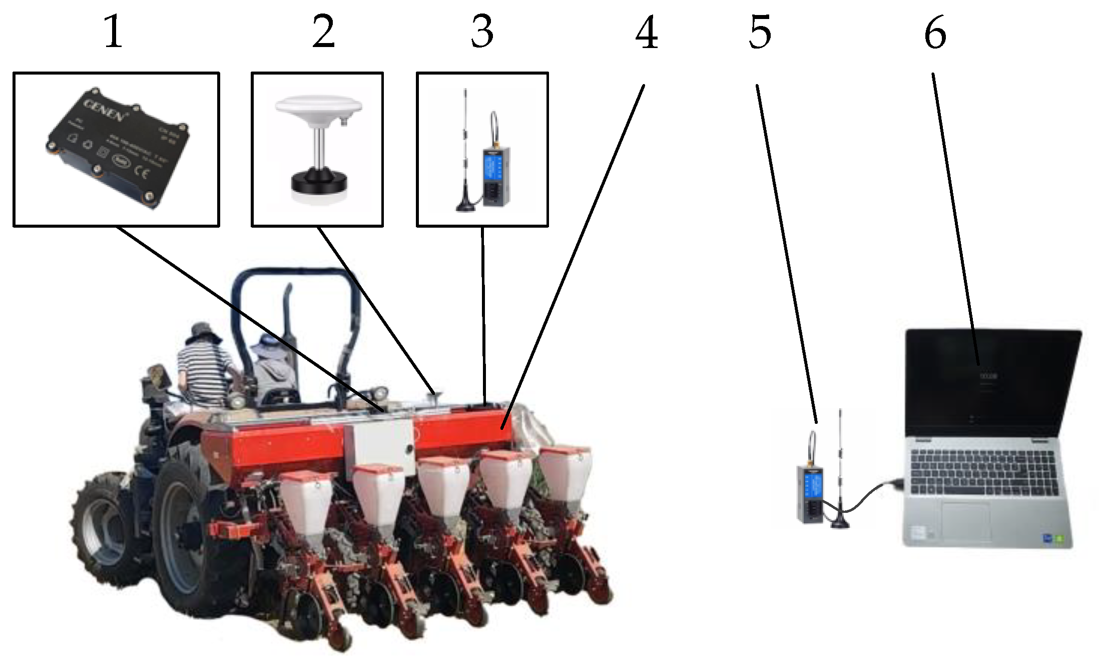
2.1. Hardware

2.1.1. Seeding Machine

In this study, a Dongfanghong ME-704 tractor suspends a wheat seeder with a 1.8 m sowing width; the RTK-GNSS positioning system is placed above the seeder on top of a vibration isolation seat; and the positioning information is communicated with a laptop computer through a wireless serial port, as shown in Figure 1. The devices that in this study deployed in Xinji, Shijiazhuang.

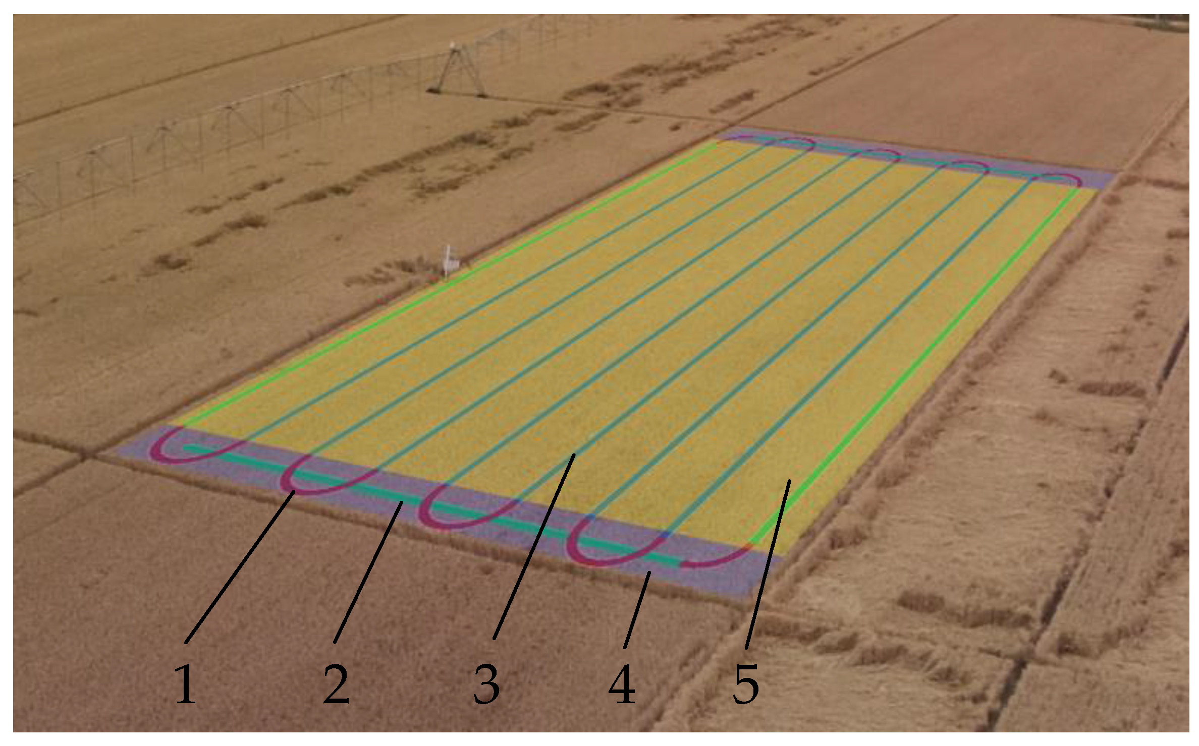
2.1.2. Trajectory Characteristics

The plot seeding operation of field crops is generally realized by reciprocating while driving parallel to one side of the border. The seeder travels in a straight line parallel to the longitudinal boundary of the farmland to sow, lifts the seeder, and turns around after reaching the horizontal plot boundary. The seeder then continues to sow in a straight line after turning around by offsetting the seeding width by one, and then repeats the above reciprocal seeding process to cover the entire longitudinal seeding area. Due to the agronomic conditions, the use of seeding equipment, and the limitations of the seeder’s own maneuverability, the seeder is not able to carry out the seeding operation when it is turned at the two ends of the plot. Therefore, after the completion of reciprocal seeding by the planter, the turnaround area is replanted, and in the turnaround area, the planter is used to seed in a straight line along the ends of the plot perpendicular to the linear seeding path. This is shown in Figure 2.

It can be summarized that the seeding path is characterized by a longitudinal seeding area, with a seeding trajectory parallel to the longitudinal boundary, a turnaround area parallel to the transverse boundary, and a straight-line seeding path enveloping the entire plot around the path. It can be seen that by extracting the peripheral envelope area of the sowing path and expanding it by half the width of the sowing width outward, an estimation of the size and orientation of the actual plot can be completed.

2.2. Boundary Extraction Based on Low-Pass Filter and Integral Clustering

Considering the characteristics of the shape of the sowing coverage boundary and the plot boundary, this paper proposes a method of estimating the plot boundary based on the shape of the sowing trajectory. The method extracts the straight-line operation trajectory by low-pass filtering and integral clustering of the radius of curvature of the trajectory points and extracts the envelope boundary of the straight-line operation area by the threshold method after the coordinate transformation of the operation trajectory according to the linear operation trajectory position, and then expands the envelope boundary to realize an accurate estimation of the plot boundary. The calculation process is shown in Figure 3.

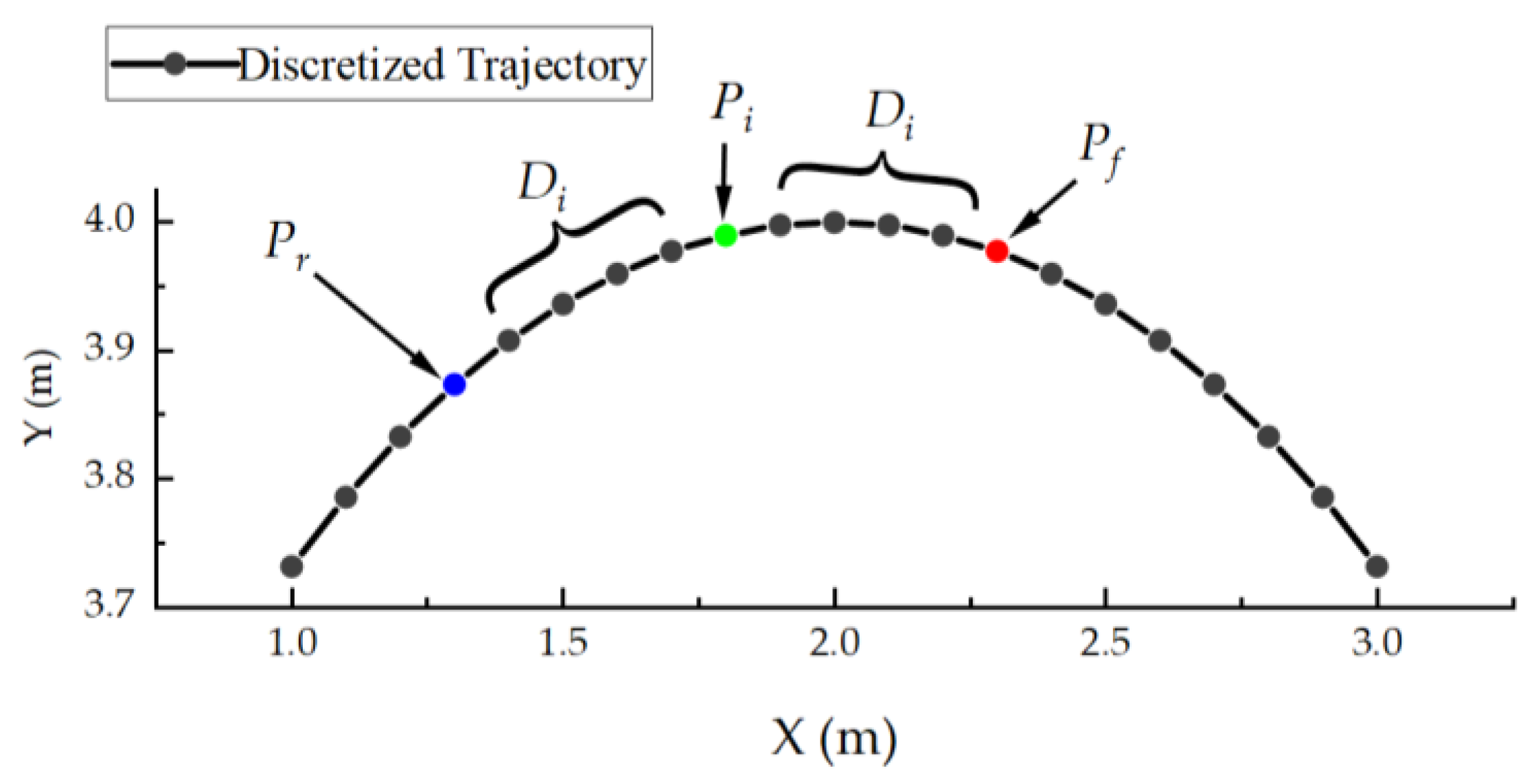
2.2.1. Path Curvature Calculation

For the discrete operational trajectory points, three points are used to calculate the curvature of the intermediate trajectory points. As shown in Figure 4, in order to calculate the curvature of the current point P_i, take the D_i point in front of P_i as P_f, and take the D_i point behind P_i as P_r. The value of D_i depends on the sampling frequency and the vehicle’s speed, which is calculated as shown in Equation (1).

$${\mathrm{D}}_{\mathrm{i}}={\displaystyle \frac{\mathrm{Freq}}{5}}$$

(1)

In this equation, Freq is the sampling frequency, divided by a constant factor, 5, which gives the curvature calculation a suitable distance.

The formula for calculating the curvature K_i at the current point is shown in Equation (2):

$${\mathrm{K}}_{\mathrm{i}}={\displaystyle \frac{\arctan \left(\frac{{\mathrm{P}}_{\mathrm{fy}}-{\mathrm{P}}_{\mathrm{iy}}}{{\mathrm{P}}_{\mathrm{fx}}-{\mathrm{P}}_{\mathrm{ix}}}\right)-\arctan \left(\frac{{\mathrm{P}}_{\mathrm{iy}}-{\mathrm{P}}_{\mathrm{ry}}}{{\mathrm{P}}_{\mathrm{ix}}-{\mathrm{P}}_{\mathrm{rx}}}\right)}{\sqrt{{\left({\mathrm{P}}_{\mathrm{ix}}-{\mathrm{P}}_{\mathrm{rx}}\right)}^2+{\left({\mathrm{P}}_{\mathrm{iy}}-{\mathrm{P}}_{\mathrm{ry}}\right)}^2}}}$$

(2)

In the formula, x and y in the corner markers of P_i and P_f represent the horizontal and vertical coordinate values of the current point.

The curvature of D_i at the insufficiently spaced points, D_i in front and behind the start and end points, is taken as the value of the curvature of the nearest point that satisfies the condition.

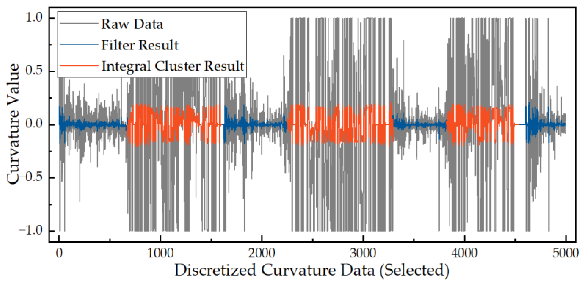
2.2.2. Discrete Data Low-Pass Filtering

In the curvature calculation, due to the noise of the positioning system and because the curvature calculation picking point interval D_i is small, a large posterior noise curvature in the curve point set exists. This original curvature waveform represents randomness and high frequency characteristics in the time domain, but the signal spectral characteristics can be directly observed in the frequency domain, and filters can be designed for the spectral characteristics. Therefore, the original curvature signal can be converted from the time domain to the frequency domain under the Fourier transform for filtering processing, to achieve the elimination of the noise signal.

The Fourier transform is shown in Equation (3):

$$\mathrm{F}\left(\mathrm{s}\right)={\int }_{-\text{∞}}^{+\text{∞}}\mathrm{f}\left(\mathrm{t}\right){\mathrm{e}}^{-\mathrm{i}\mathrm{s}\mathrm{t}}\mathrm{d}\mathrm{t}$$

(3)

The low-pass filter transfer function is shown in Equation (4):

$$\mathrm{H}\left(\mathrm{s}\right)={\displaystyle \frac{{\mathsf{\omega }}_0}{\mathrm{s}+{\mathsf{\omega }}_0}}$$

(4)

where ω₀ is the system cutoff frequency.

If the system sampling frequency is assumed to be f_s, and Δt is the sampling duration, the discretized system step size is shown in Equation (5):

$$\mathsf{\Delta }\mathrm{t}={\displaystyle \frac{1}{{\mathrm{f}}_{\mathrm{s}}}}$$

(5)

The s is bilinearly transformed as shown in Equation (6):

$$\mathrm{H}\left(\mathrm{z}\right)={\displaystyle \frac{\mathsf{\Delta }\mathrm{t}{\mathsf{\omega }}_0\left(\mathrm{z}+1\right)}{\left(\mathsf{\Delta }\mathrm{t}{\mathrm{w}}_0+2\right)\mathrm{z}+\mathsf{\Delta }\mathrm{t}{\mathsf{\omega }}_0-2}}$$

(6)

Its constant coefficient differential equation is shown in Equation (7):

$$\mathrm{H}\left(\mathrm{z}\right)={\displaystyle \frac{{\mathrm{b}}_0+{\mathrm{b}}_1{\mathrm{z}}^{-1}+{\mathrm{b}}_2{\mathrm{z}}^{-2}+\text{…}}{1-{\mathrm{a}}_1{\mathrm{z}}^{-1}-{\mathrm{a}}_2{\mathrm{z}}^{-2}+\text{…}}}$$

(7)

A and b are the factor of coefficient differential equation, extracting the factor using the equation below to create the filter.

The differential equation of the complete filter is modeled as Equation (8):

$$\mathrm{y}\left[\mathrm{n}\right]={\mathrm{a}}_1\mathrm{y}\left[\mathrm{n}-1\right]+{\mathrm{b}}_0\mathrm{x}\left[\mathrm{n}\right]+{\mathrm{b}}_1\mathrm{x}\left[\mathrm{n}-1\right]$$

(8)

where y [n] is the filtered discrete curvature value result and x [n] is the discretized system raw data.

2.2.3. Integral Clustering

The mapping of the curvature values of the straight line and the turnaround path of the seeding vehicle to the discrete data in the time domain shows that the curvature values close to 0 alternate with the values along with jumps in the form of turnarounds and straight-line travel. However, there are still some anomalies in the actual curvature values in the turn curvature point set, due to sensor noise and filtering performance limitations. In order to be able to completely extract the curve path point set, this paper proposes an integral clustering algorithm; traversing all the path points, the current point after the step length of Δs contained in the discrete point set value for the curvature value integral calculation, as shown as Equation (9):

$$\mathrm{G}\left(\mathrm{i}\right)={\int }_{\mathrm{p}}^{\mathrm{p}+\mathsf{\Delta }\mathrm{s}}\mathrm{y}\left(\mathrm{i}\right)\mathrm{d}\mathrm{t}$$

(9)

In Equation (9), y(i) represents the curvature value after the filter, p is the discrete point index, and Δs is the integral length. Obviously, the curvature of the curve is greater than that of the straight line. When the value of G(i) is greater than the threshold S, it represents that the curvature of the path form of the current point set conforms to the steering curvature form and marks all the points within this integral step as a steering point set, otherwise it is marked as a linear point set.

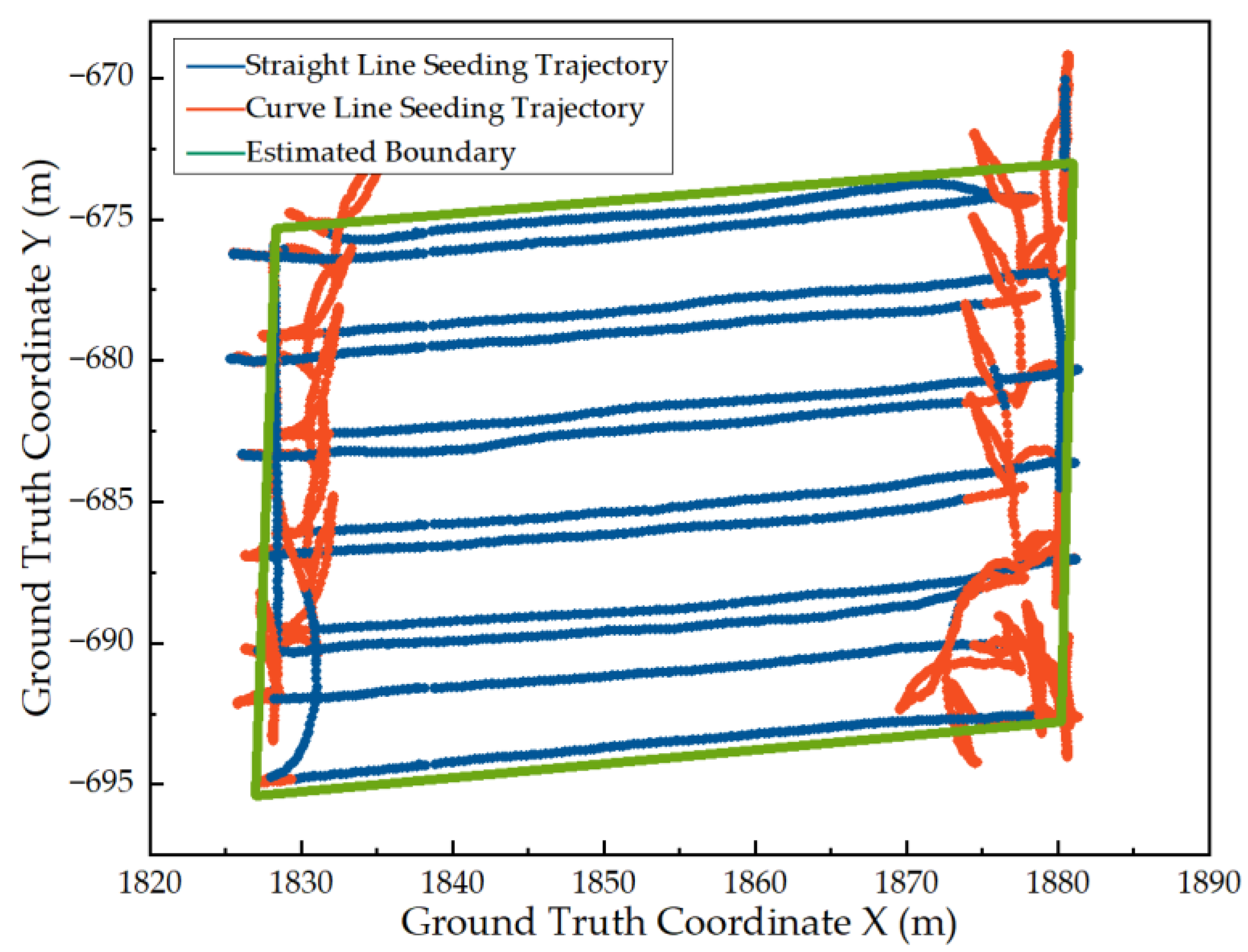
2.2.4. Orthogonal Rotation of Seeding Paths

Due to the different orientations of the seeding plots, the linear part of the seeding path is not orthogonal to the computed coordinate system, which creates some difficulties in determining the envelope path. Therefore, it is necessary to judge the orientation of the seeding paths and rotate the paths to the orthogonal state of the coordinate axes to facilitate the search for edge paths.

The seeder mainly works in straight-line seeding, and according to this characteristic, all the path point headings are distinguished and counted, and the number of all the path point headings is counted with the resolution of R degree. The point set headings with the highest number of counts is determined as the plot facing Dir.

In order to rotate the path points to be orthogonal to the coordinate axes, the angle at which the path points need to be rotated can be calculated using Equation (10).

$$\mathsf{\theta }={\displaystyle \frac{\mathsf{\pi }}{2}}-\mathrm{Dir}$$

(10)

If you define the coordinates of a point before rotation to be x, y; after rotation to be x′, y′; and the coordinates of a point heading before rotation to be phi; and after rotation to be phi′, its rotation matrix is as shown in Equation (11):

$$\left[\begin{array}{c}{\mathrm{x}}^{\prime }\\ {\mathrm{y}}^{\prime }\\ \mathrm{p}\mathrm{h}{\mathrm{i}}^{\prime }\end{array}\right]=\left[\begin{array}{ccc}\cos \mathsf{\theta }& -\sin \mathsf{\theta }& 0\\ \mathrm{s}\mathrm{in}\mathsf{\theta }& \cos \mathsf{\theta }& 0\\ 0& 0& 1\end{array}\right]\left[\begin{array}{c}\mathrm{x}\\ \mathrm{y}\\ \mathrm{p}\mathrm{h}\mathrm{i}\end{array}\right]+\left[\begin{array}{c}0\\ 0\\ \mathsf{\theta }\end{array}\right]$$

(11)

2.2.5. Orthogonal Rotation of Seeding Paths

For the path points that are orthogonal to the coordinate system, the point sets that are labeled as a straight line by the cluster analysis, the point position is at the edge of all the path locations. The total number of consecutively arranged path points before and after the point is greater than a certain number of P and is determined to be the edge of the plot envelope path. Take the rightmost boundary path as an example, when the x coordinate value of the point set is larger than all of the coordinate points in the point set, and the P points before and after this point are all straight lines, then this continuous straight line point set is determined as the rightmost envelope path.

The set of envelope path points is subjected to a one-dimensional linear fitting process. The objective is to find a linear equation as in Equation (12):

$${\mathrm{y}}_{\mathrm{i}}={\mathrm{c}}_1{\mathrm{x}}_{\mathrm{i}}+{\mathrm{c}}_0$$

(12)

Each point on a straight line minimizes the sum of distances from this linear equation. The above equation can then be rewritten in matrix form as shown in Equation (13):

$$\left[\begin{array}{cc}1& {\mathrm{x}}_1\\ 1& {\mathrm{x}}_2\\ \text{⋮}& \text{⋮}\\ 1& {\mathrm{x}}_{\mathrm{n}}\end{array}\right]\left[\begin{array}{c}{\mathrm{c}}_0\\ {\mathrm{c}}_1\end{array}\right]=\left[\begin{array}{c}{\mathrm{y}}_1\\ {\mathrm{y}}_2\\ \text{⋮}\\ {\mathrm{y}}_{\mathrm{n}}\end{array}\right]$$

(13)

Rewrite this as Equation (14):

$$\mathrm{Xc}=\mathrm{y}$$

(14)

Since y is not in the column vector space of X, there is no solution to this equation; therefore consider its approximate solution. Project y into the column vector space of X as in Equation (15):

$$\mathrm{Xb}=\widehat{\mathrm{y}}$$

(15)

Here, if $\widehat{y}$ is the projection of y, b is a projection factor.

At this point, let the projection matrix P be Equation (16):

$$\mathrm{P}=\mathrm{X}{\left({\mathrm{X}}^{\mathrm{T}}\mathrm{X}\right)}^{-1}{\mathrm{X}}^{\mathrm{T}}$$

(16)

i.e., Equations (17) and (18):

$$\widehat{\mathrm{y}}=\mathrm{Py}=\mathrm{X}{\left({\mathrm{X}}^{\mathrm{T}}\mathrm{X}\right)}^{-1}{\mathrm{X}}^{\mathrm{T}}\mathrm{y}=\mathrm{Xb}$$

(17)

$$\mathrm{b}={\left({\mathrm{X}}^{\mathrm{T}}\mathrm{X}\right)}^{-1}{\mathrm{X}}^{\mathrm{T}}\mathrm{y}$$

(18)

Expanding the matrix X results in the final linear coefficients, as shown in Equation (19):

$$\mathrm{b}=\left[\begin{array}{c}\stackrel{\mathrm{-}}{\mathrm{y}}-{\mathrm{b}}_1\stackrel{\mathrm{-}}{\mathrm{x}}\\ {\displaystyle \frac{\sum \left({\mathrm{x}}_{\mathrm{i}}-\stackrel{\mathrm{-}}{\mathrm{x}}\right)\left({\mathrm{y}}_{\mathrm{i}}-\stackrel{\mathrm{-}}{\mathrm{y}}\right)}{\sum {\left({\mathrm{x}}_{\mathrm{i}}-\stackrel{\mathrm{-}}{\mathrm{x}}\right)}^2}}\end{array}\right]$$

(19)

in matrix b are the slope and intercept of the line on which they are located, respectively.

2.2.6. Orthogonal Rotation of Seeding Paths

The results of the univariate linear fitting for all four boundaries are the traveling position of the center of the seeder. The real plot boundaries, on the other hand, need to be extended outward by half the width of the seeding width in the vertical direction of the seeding path. Assume that the linear equation fitted to the left boundary is Equation (20):

$$\mathrm{y}=\mathrm{kx}+\mathrm{b}$$

(20)

Extend the distance L to the left by changing b to b′ in the original linear equation, which is calculated as Equation (21):

$${\mathrm{b}}^{\prime }=\mathrm{b}+\sqrt{\left(1+{\mathrm{k}}^2\right)\text{×}{\mathrm{L}}^2}$$

(21)

Similarly, the remaining three boundaries can be calculated.

Finally, the four calculated boundaries are intersected two by two, and the four calculated plot vertices and the four straight lines are the results of the estimated plot size orientation.

3. Results

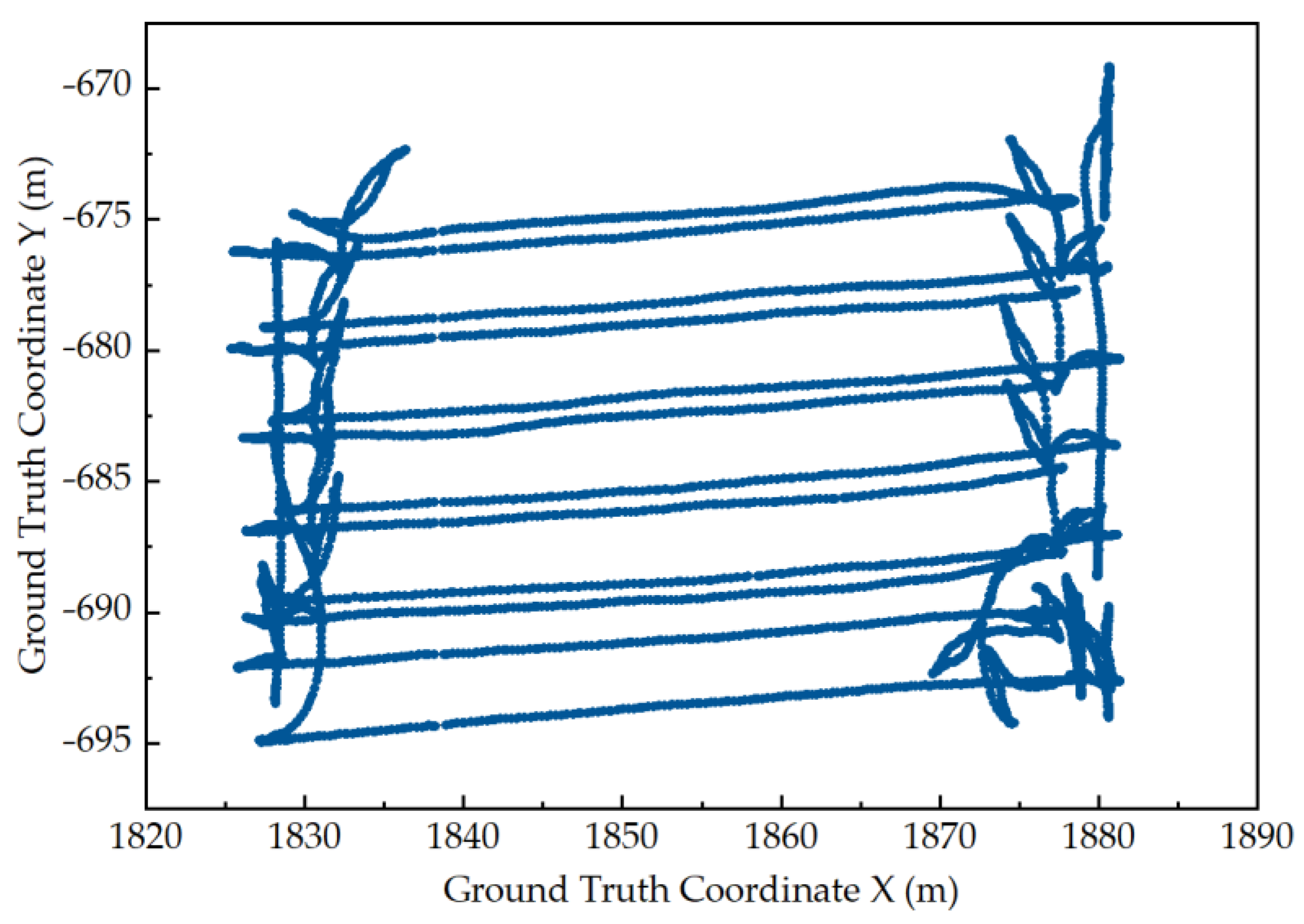
3.1. Trajectory Data Acquisition

The speed of the tractor at the time of seeding is 0.8 m/s, the data acquisition frequency of the positioning system is 20 Hz, and acquired information includes the relative horizontal and vertical coordinates of the seeder x and y, and the heading angle phi. The seeding path acquisition data is shown in Figure 5.

3.2. Calculating Results

Using the methodology presented in Section 2.2, the parameters applied to the above data for morphological curvature calculation, low-pass filtering, integral clustering, and parcel boundary estimation are shown in

Table 1. Algorithm Parameters.

Parameter Name	Value
Curvature Calculation Points Interval Di	5
System Cut-off Frequency ω0	2π
Integral Step Length Δs	100
Integral Threshold S	8
Heading Resolution R	0.1
Continuous Boundary Dots Set Amount P	100

.

The above data were low-pass filtered, and part of the results are shown in Figure 6. The gray line in the figure are the original curvature values, the blue and orange line combination is the curvature values after low-pass filtering, and the orange lines are the points that were integral clustered as curves from the filtered data.

Trajectories were plotted using the clustering results in Figure 6, as shown in Figure 7, where the blue color is the straight-line seeding trajectory; the orange color is the curved turn-around trajectory; and the green color is the result of the plot boundary estimation.

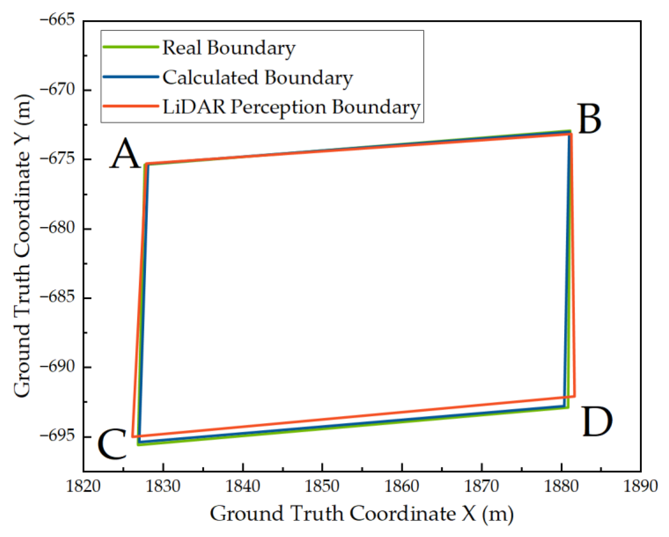
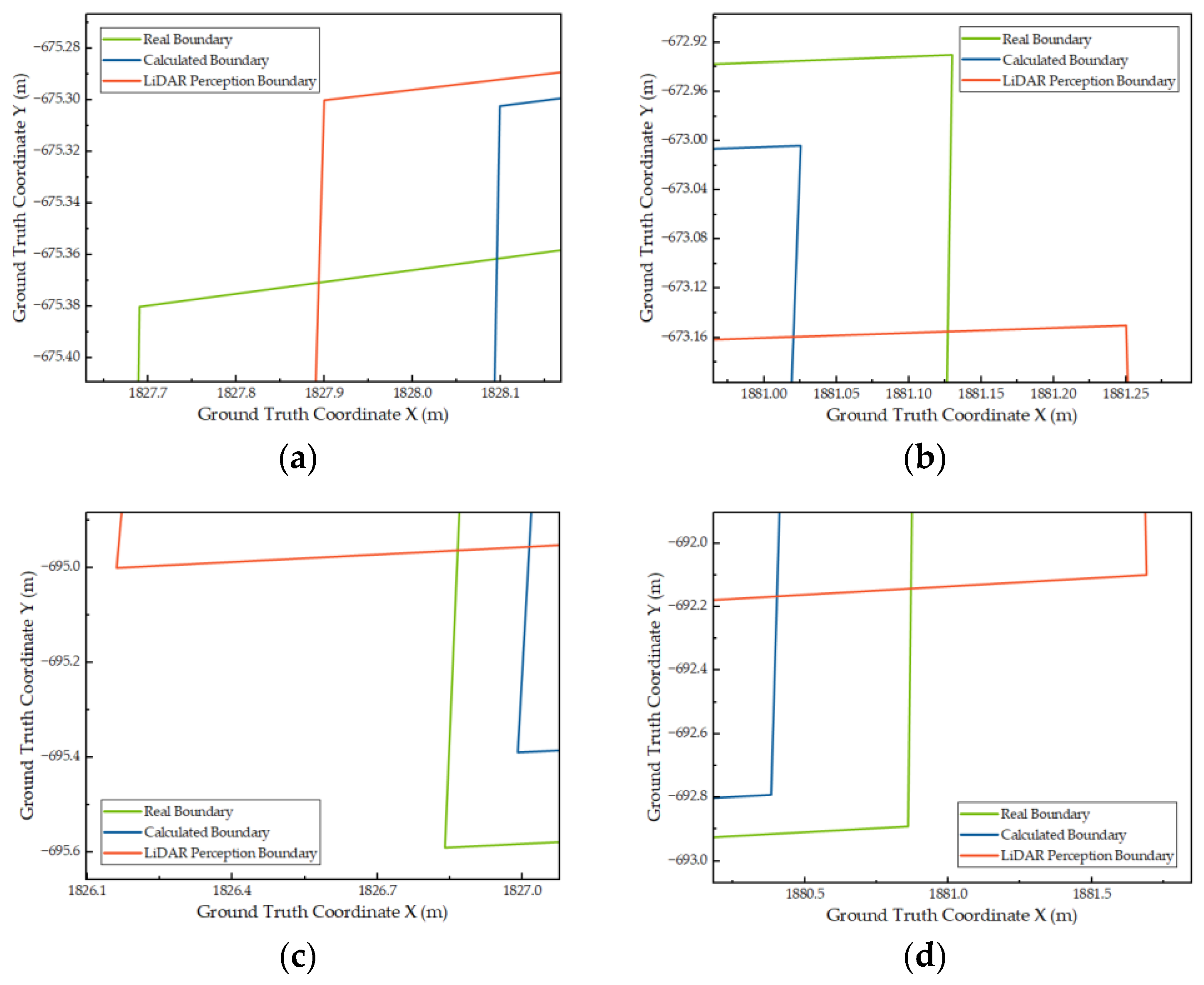
3.3. Results Comparison

In order to verify the accuracy and feasibility of this method, the actual boundaries of the plots were compared using three methods: trajectory estimated boundaries, LiDAR scanning to obtain plot boundaries, and manual GPS pointing.

The LiDAR scanning and computational processing to obtain the estimated boundary of the parcel is shown in Figure 8. The LiDAR was fixed on the front top of the tractor, using tractor wheel odometry and an imu and LiDAR point cloud ICP fusion to map the farmland.

The handheld GPS puncturing method to acquire the actual plot boundary, the LiDAR computational processing to acquire the boundary, and the plot boundary estimation to acquire the boundary comparison are shown in Figure 9.

As can be seen in Figure 9, all methods are able to acquire the boundary of the farmland, and considering that the hand-held GPS point is used as the actual reference boundary, the plot boundary acquired by trajectory estimation is obviously closer to the actual boundary of the plot than the boundary acquired by LiDAR.

The four vertices of the plot are A, B, C, and D. The detailed coordinate positions of the vertices in the coordinate system are shown in Figure 10 and

Table 2. Corner point coordinates (in meters).

Corner	Real Boundary		Calculated Boundary		LiDAR Perception Boundary
	X	Y	X	Y	X	Y
A	1827.69	−675.38	1828.09	−675.30	1827.90	−675.30
B	1881.13	−672.93	1881.02	−673.00	1881.25	−673.15
C	1826.84	−695.59	1826.99	−695.38	1826.16	−695.00
D	1880.86	−692.89	1880.38	−692.79	1881.69	−693.26

.

Taking the manual measurement of the vertex position as a benchmark, it can be calculated from the data in the table that, in terms of the vertex straight line distance error, the LiDAR achieves a maximum error of 1.14 m at point D, the minimum error is 0.22 m at point A, and the average straight line distance error of the four-corner vertices is 0.63 m; the maximum, minimum, and average errors calculated by the trajectory estimation are 0.48 m at point C, 0.12 m at point B, and 0.32 m, respectively.

In terms of the boundary straight line, the detection results of the LiDAR CD section has an obvious overall offset; the average error is 0.62 m. The AC and BD sections have a more obvious angular deviation at, respectively, 2.1 degrees and 1.9 degrees; for the trajectory estimation results, the BD section has the most obvious overall offset, the average error is 0.11m, and the maximum angular deviation in the BD section is 1.56 degrees.

The area of the handheld GPS punched trajectory was 1077.72 m².

Table 3. Estimation of area results (in m²).

	LiDAR Perception	Trajectory Estimation
Calculated area	1048.52	1061.10
Missing area	41.49	17.64
Exceeded area	12.27	1.02

summarizes the statistics of the plot area of the LiDAR and trajectory estimation methods and compares this with the actual plot area.

In the table above, the dimensional orientation of the plots obtained by manual punching is the base plot, and the uncovered area is the missed area; the area of the estimated plots beyond the base plot is the overflow area. In terms of the estimated area, the trajectory estimation method is closer to the real result of 1077.72 m², with an estimated result of 1061.10 m² compared to the 1048.52 m² obtained using LiDAR. In terms of the missed area and the overflow area, the 17.64 m² and 1.02 m² results of the trajectory estimation method are better than the 41.49 m² and 12.27 m² results using LiDAR.

In terms of the computational consumption, for example, the total amount of data collected is 24,596 points, and the total running time of this program is 5.4 × 10⁻⁴ s for a computer equipped with CPU model i7-11800H; the total number of floating-point calculations is about 1.2 megaflops. LiDAR map building requires a high real-time capacity and the total running time is more difficult to count, but the total consumption of floating-point calculation amount is about 4.8 G times.

3.4. Results Analysis

In terms of average error, the trajectory is estimated to be 0.32 m, which is 50.23% of the 0.627 m trajectory estimate using LiDAR; in terms of linear error at the boundary, compared with the average 0.62 m translation deviation of LiDAR detection results, the average error of trajectory estimation is 0.11 m, which is only 17.74% of the LiDAR error. In terms of estimating the overflow area, LiDAR overflows the actual parcel by 12.27 m², while this algorithm spills into a very little area, only 1.02m²; in terms of the missed area, LiDAR and the method used in this paper have a similar effect in terms of the overflow area, which is only 1.02 m². In terms of area, both LiDAR and the calculation method of this paper have certain omissions, respectively 41.49 m² and 17.64 m²; the estimation method proposed in this paper has 23.85 m² less omissions than LiDAR. In terms of the estimated area overlap rate, the trajectory estimates an area overlap rate of 98.36%, which is 2.21% higher than that of LiDAR; in terms of the computational consumption, the algorithmic program in this paper completes the estimation of plot size and orientation with only 1.2 trillion floating point operations, which is one-fourth of the 4.8 G floating point operations consumed by the LiDAR map building program.

4. Discussion

In this study, due to the individual driving habits of the tractor driver, the trajectory shows the pattern seen in Figure 5 when turning around on the ground.

The path curvature calculation is based on discrete points, and when the tractor switches the traveling direction forwards and backwards, the calculated curvature value may be extremely large or small. Although the threshold value is added in this paper, there are still some values that do not reach the threshold clamp range but are still higher than the curvature value of a straight line or a general curve. When selecting points for the curvature calculation, either too large or too small spacing between points will have some effect on the curvature calculation. Too small point spacing will amplify the positioning system noise indefinitely, while too large spacing will result in a severe lag and a distortion in the curvature calculation.

In the final integral clustering used to distinguish curvature, the choice of the integral threshold is critical, and the size of the threshold directly affects how accurate the point set is. Too small a threshold may result in most point sets being judged as curves, and vice versa. The parameters used in this study have been optimized through many iterations, and are better adapted to the morphological differentiations in the seeding trajectories in this study.

5. Conclusions

In this study, a plot boundary estimation method based on seeding paths is proposed. The method firstly calculates the morphological curvature of the seeding path, and then low-pass filters acquire the curvature values; subsequently, thresholds are calculated from the filtered curvature values for integral clustering to differentiate between straight lines and curves, and finally a one-dimensional linear fitting of the edge straight-line path points is performed to obtain the boundaries of the operational plots; an innovative use of path data for estimation of plot boundaries.

Through the field tests, it can be seen that in the trajectory estimation of the farmland plots, the minimum straight-line distance error of the vertices of the plots is only 0.12 m, and the coincidence rate of the plot estimation is as high as 98.36%; although there is still a certain size and orientation deviation between the estimated plots and the actual operation plots, it can still be used as digital mapping data for the agricultural automation equipment.

The method proposed in this study has a simple demand for data sources, which requires only the seeding path of agricultural machines and does not rely on other complex sensors to complete the estimation of the plots; the trajectory estimation has a low demand for computational power, which requires only about 1.2 megawatt floating-point operations to complete the estimation of the boundary of the path, using more than 10,000 path points and more than 1000 square meters of seeding plot paths. When calculating the curvature of the path, a more accurate curvature calculation method is proposed, and the curvature value characteristics can be clustered with the integral values, which can be used to distinguish between the straight-line and curved-line parts of the discrete path data.

However, this method is only effective for rectangular plots with a single plot boundary, and further research is needed for other shaped plots and undulating plots. When analyzing seeding paths, other sensors can be integrated to distinguish between straight and curved paths more accurately and clearly, thus further improving the estimation accuracy.

References

1. Zhao, C. Current situations and prospects of smart agriculture. J. South China Agric. Univ. 2021, 42, 1–7. [Google Scholar]
2. Zhao, C. State-of-the-art and recommended developmental strategic objectives of smart agriculture. Smart Agric. 2019, 1, 1–7. [Google Scholar]
3. Kamilaris, A.; Kartakoullis, A.; Prenafeta-Boldú, F.X. A Review on the Practice of Big Data Analysis in Agriculture. Comput. Electron. Agric. 2017, 143, 23–37. [Google Scholar] [CrossRef]
4. Wang, T.; Xu, X.; Wang, C.; Li, Z.; Li, D. From Smart Farming towards Unmanned Farms: A New Mode of Agricultural Production. Agriculture 2021, 11, 145. [Google Scholar] [CrossRef]
5. Ma, Z.; Chong, K.; Zhao, X.; Zhao, J.; Zhao, S.; Yu, H. Research on the work precision of farm machinery driven by automatic navigation tractors. J. Hebei Agric. Univ. 2022, 45, 109–114. [Google Scholar] [CrossRef]
6. Lu, B.; Dong, W.; Ding, Y.; Sun, Y.; Li, H.; Zhang, C. An rapeseed unmanned seeding system based on cloud-terminal high precision maps. Smart Agric. 2023, 5, 33–44. [Google Scholar]
7. Ju, J.; Chen, G.; Lv, Z.; Zhao, M.; Sun, L.; Wang, Z.; Wang, J. Design and Experiment of an Adaptive Cruise Weeding Robot for Paddy Fields Based on Improved YOLOv5. Comput. Electron. Agric. 2024, 219, 108824. [Google Scholar] [CrossRef]
8. Zhao, C.; Fan, B.; Li, J.; Feng, Q. Technology progress, challenges and trends. Smart Agric. 2023, 5, 1–15. [Google Scholar]
9. Wang, N.; Yang, X.; Wang, T.; Xiao, J.; Zhang, M.; Wang, H.; Li, H. Collaborative Path Planning and Task Allocation for Multiple Agricultural Machines. Comput. Electron. Agric. 2023, 213, 108218. [Google Scholar] [CrossRef]
10. Zhang, Y. Monitoring maize evapotranspiration and soil water content in farmland based on UAV multi-source remote sensing data. Ph.D. Thesis, Research Center of Soil and Water Conservation and Ecological Environment, Chinese Academy of Sciences and Ministry of Education, Xianyang, China, 2024. [Google Scholar]
11. Xu, J.; Liu, Y.; Yan, C.; Yuan, J. Estimation of Soil Organic Matter Based on Spectral Indices Combined with Water Removal Algorithm. Remote Sens. 2024, 16, 2065. [Google Scholar] [CrossRef]
12. Zhang, K.; Gong, L.; He, Z.; Huo, P. Crop yield prediction based on 3DCNN-TCN model. Microelectron. Comput. 2023, 40, 83–89. [Google Scholar] [CrossRef]
13. Wang, H.; Ma, Z.; Ren, Y.; Du, S.; Lu, H.; Shang, Y.; Hu, S.; Zhang, G.; Meng, Z.; Wen, C.; et al. Interactive Image Segmentation Based Field Boundary Perception Method and Software for Autonomous Agricultural Machinery Path Planning. Comput. Electron. Agric. 2024, 217, 108568. [Google Scholar] [CrossRef]
14. Chen, L.; Si, Y.; Tian, B.; Tan, Z.; Wang, Y. Boundary detection of mine drivable area based on 3D LiDAR. J. China Coal Soc. 2020, 45, 2140–2146. [Google Scholar] [CrossRef]
15. Zhan, J.; Guo, C.; Lei, T.; Qu, Y.; Wu, H.; Liu, J. Comparative study on data standards of autonomous driving map. J. Image Graph. 2021, 26, 36–48. [Google Scholar]
16. Ma, Z.; Chong, K.; Ma, S.; Fu, W.; Yin, Y.; Yu, H.; Zhao, C. Control Strategy of Grain Truck Following Operation Considering Variable Loads and Control Delay. Agriculture 2022, 12, 1545. [Google Scholar] [CrossRef]
17. Aguiar, A.S.; dos Santos, F.N.; Cunha, J.B.; Sobreira, H.; Sousa, A.J. Localization and Mapping for Robots in Agriculture and Forestry: A Survey. Robotics 2020, 9, 97. [Google Scholar] [CrossRef]
18. Liu, Z. Research on Visual Slam of Inspection Robot Based on Image Defogging and Semantic Mapping. Master Thesis, Shandong University, Jinan, China, 2021. [Google Scholar]
19. Wagner, M.P.; Oppelt, N. Deep Learning and Adaptive Graph-Based Growing Contours for Agricultural Field Extraction. Remote Sens. 2020, 12, 1990. [Google Scholar] [CrossRef]
20. Gafurov, A. Automated Mapping of Cropland Boundaries Using Deep Neural Networks. AgriEngineering 2023, 5, 1568–1580. [Google Scholar] [CrossRef]
21. Borowiec, N.; Marmol, U. Using LiDAR System as a Data Source for Agricultural Land Boundaries. Remote Sens. 2022, 14, 1048. [Google Scholar] [CrossRef]
22. Zhang, Y.; Li, Y.; Liu, X.; Tao, J.; Liu, C.; Li, R. An Automatic Drive Control Technique for Rice Drill Seeder in Uneven Paddy Fields. Trans. Chin. Soc. Agric. Mach. 2018, 49, 15–22. [Google Scholar]
23. Cai, D.; Li, Y.; Qin, C.; Liu, C. Detection Method of Boundary of Paddy Fields Using Support Vector Machine. Trans. Chin. Soc. Agric. Mach. 2019, 50, 22–27. [Google Scholar]
24. Zhai, W.; Xiong, X.; Mo, G.; Xiao, Y.; Wu, C.; Xu, Z.; Pan, J. A Bagging-SVM Field-Road Trajectory Classification Model Based on Feature Enhancement. Comput. Electron. Agric. 2024, 217, 108635. [Google Scholar] [CrossRef]
25. He, X.; Zhu, J.; Li, P.; Zhang, D.; Yang, L.; Cui, T.; Zhang, K.; Lin, X. Research on a Multi-Lens Multispectral Camera for Identifying Haploid Maize Seeds. Agriculture 2024, 14, 800. [Google Scholar] [CrossRef]
26. Li, Q.; Zhu, H. Performance Evaluation of 2D LiDAR SLAM Algorithms in Simulated Orchard Environments. Comput. Electron. Agric. 2024, 221, 108994. [Google Scholar] [CrossRef]
27. Naich, A.Y.; Carrión, J.R. LiDAR-Based Intensity-Aware Outdoor 3D Object Detection. Sensors 2024, 24, 2942. [Google Scholar] [CrossRef]
Figure 1. Seeding and recording hardware. Note: 1. RTK Chip; 2. GNSS Antenna; 3. Wireless Serial Data Sender; 4. Seeding Machine; 5. Wireless Serial Data Receiver; 6. Laptop.
Agriculture 14 01238 g001
Figure 2. Schematic diagram of seeding method. Note: 1. Red, U-turn trajectory; 2. Green, boundary and straight line seeding trajectory; 3. Blue, straight line seeding trajectory; 4. Blue area, U-turn and additional seeding area; 5. Yellow area, normal seeding area.
Agriculture 14 01238 g002
Figure 3. Method flow chart.
Agriculture 14 01238 g003
Figure 4. Discrete trajectory curvature calculation.
Agriculture 14 01238 g004
Figure 5. Seeding trajectory.
Agriculture 14 01238 g005
Figure 6. Curvature, filtering and integration of discrete data.
Agriculture 14 01238 g006
Figure 7. Trajectory clustering and plot boundary estimation results.
Agriculture 14 01238 g007
Figure 8. LiDAR point cloud.
Agriculture 14 01238 g008
Figure 9. Boundary estimation comparation.
Agriculture 14 01238 g009
Figure 10. Boundary corners. (a) upper left corner; (b) upper right corner; (c) bottom left corner; (d) bottom right corner.
Agriculture 14 01238 g010